Above- and Belowground Biomass Models for Trees in the Miombo Woodlands of Malawi

Abstract

In this study we present general (multiple tree species from several sites) above- and belowground biomass models for trees in the miombo woodlands of Malawi. Such models are currently lacking in the country. The modelling was based on 74 trees comprising 33 different species with diameters at breast height (dbh) and total tree height (ht) ranging from 5.3 to 2 cm and from 3.0 to 25.0 m, respectively. Trees were collected from four silvicultural zones covering a wide range of conditions. We tested different models including dbh, ht and wood specific gravity ($\mathsf{\rho }$) as independent variables. We evaluated model performance using pseudo-R², root mean square error (RMSE), a covariance matrix for the parameter estimates, mean prediction error (MPE) and relative mean prediction error (MPE%). Computation of MPE% was based on leave-one-out cross-validation. Values of pseudo-R² and MPE% ranged 0.82–0.97 and 0.9%–2.8%, respectively. Model performance indicated that the models can be used over a wide range of geographical and ecological conditions in Malawi.

1. Introduction

Miombo woodlands, classified as dry forests, are dominated by woody plants, primarily trees, whose canopy cover more than 10% of the ground surface, occurring in a climate with a dry season of three months or more [1]. The woodlands are dominated by deciduous trees of the genera Brachystegia, Julbernadia and Isoberlinia, which cover an area of approximately 2.7 million km² spanning ten countries in eastern and central Africa including Malawi [1,2,3,4,5]. Miombo woodlands may be divided into dry and wet miombo. Dry miombo occur in areas receiving less than 1000 mm of rainfall annually in Zimbabwe, central Tanzania, and in the southern areas of Mozambique, Malawi and Zambia. Wet miombo occur in areas receiving more than 1000 mm of annual rainfall in eastern Angola, northern Zambia, south western Tanzania and central Malawi [1,6]. In Malawi, miombo woodlands constitute 92.4% of the country’s total forested area, and are mainly located in forest and game reserves established for water catchment as well as for soil and biodiversity conservation [2,7].

Miombo woodlands play a critical role in the livelihoods of Malawian communities because they provide social, economic, and environmental benefits, such as firewood, timber, medicinal plants, food, and catchment protection, among others [8]. Increased population growth, currently estimated at an annual growth rate of 2.8% [9], has led to higher demand for firewood, charcoal, and timber. Thus, the woodlands are being deforested at an annual rate of approximately 0.9%, which is among the highest rates in Africa [10].

To sustain the provision of these services, there is an urgent need to implement sustainable forest management measures including estimation of growing stock, productivity, forest biomass and yield [11,12]. Estimation of forest biomass is the first step towards calculation of carbon stocks. Due to the natural capacity of trees to sequester carbon dioxide, miombo woodlands are considered an important element in global climate change mitigation programs such as the reducing emissions from deforestation and forest degradation mechanism (REDD+), which provides a framework where developing countries may be financially rewarded for reducing carbon emissions.

The Malawi government recently established a baseline for forest biomass and carbon stock estimates for targeted forest reserves in miombo woodlands of Malawi [7]. However, the estimates are unreliable because of the nature of the allometric models that were used. For example, the aboveground forest biomass estimates were based on a pan-tropical biomass model developed by Chave et al. [13]. This model was developed using data from trees in tropical America and Asia but did not include Africa or the miombo woodlands. In addition, belowground forest biomass estimates were based on an allometric model developed by Cairns et al. [14]. Unlike Chave et al. [13], this dataset included some trees from Africa, i.e., Democratic Republic of the Congo, Ghana and the Ivory Coast. However, the trees were from moist evergreen tropical forests, whose structure is different from miombo woodlands.

By 2011 there were approximately 370 allometric models for predicting tree biomass in sub-Saharan Africa [15]. The majority of these models were developed for tropical rainforests in western Africa. Among the models in south-eastern Africa, only a few were developed for miombo woodlands. These models consisted of: (a) models developed for specific tree species based on a dataset from one site (Mwakalukwa et al. [16]); (b) models developed for specific tree species based on a dataset from several sites (Mate et al. [17]); (c) models developed for multiple tree species based on a dataset from one site (Chidumayo [18], Chamshama et al. [19], Malimbwi et al. [20], Ryan et al. [4], Mwakalukwa et al. [16]) and (d) models developed for multiple tree species based on a dataset from several sites (Mugasha et al. [21]).

Miombo woodlands are characterized by high tree species diversity, and the reported number of species from assessments at different spatial scales ranges from 80 to 300 [22,23,24,25,26,27]. Due to such large number of tree species, the applicability of species-specific models is limited. Furthermore, applicability of single-site models over different ecological zones is also limited due to their narrow geographical range. A scenario with general models, combining multiple species collected over several sites, would therefore be the best alternative, for example, in cases where national forest inventories are to be carried out. No such models exist for miombo woodlands in Malawi.

Most of the previously mentioned studies focused on aboveground biomass. However, estimation of belowground biomass in miombo woodlands is also vital. Belowground tree biomass, as a basis for model development, can be determined using complete excavation of roots, soil core sampling for fine and medium roots, and root sampling (complete excavation of a few sampled roots of a tree). Estimating belowground tree biomass can be done by using the root to shoot ratio (RS-ratio), i.e., the ratio between belowground and aboveground dry weights (see e.g., [28,29]), or through allometric models. Belowground biomass models for miombo woodlands in neighbouring countries were developed by Mugasha et al. [21], Chidumayo [18] and Ryan et al. [4].

The Inter-governmental Panel on Climate Change (IPCC) (see [30]) requires biomass and carbon reporting under the REDD+ mechanism to be accompanied by appropriate measures of uncertainty. Uncertainties are likely to occur in the following steps in biomass quantification: (i) when applying the sampling design (number and size of plots); (ii) during tree measurements and (iii) when applying the biomass model (e.g., [31,32]). The model-related uncertainty in this context stems from sources such as: (a) model misspecifications; (b) uncertainties in values of independent variables; (c) residual variability and (d) uncertainty in the model parameter estimates (see e.g., [33,34]). Among these, uncertainty in model parameter estimates has a great influence [35]. However, very few studies report uncertainty in the model parameter estimates, i.e., the covariance structure of the parameter estimates of developed models, and this makes it impossible to analyse the totality of the uncertainty related to estimated forest biomass (see [35]).

The objective of this study is to develop general (multiple tree species from several sites) above- and belowground biomass models applicable across the entire distribution of miombo woodlands in Malawi. The models are also accompanied with information on their covariance structure to enable quantification of model-related uncertainties in biomass and carbon estimation. Furthermore, we provide basic statistics on RS-ratios and compare the performance of our models with existing models from miombo woodlands.

2. Materials and Methods

2.1. Site Description

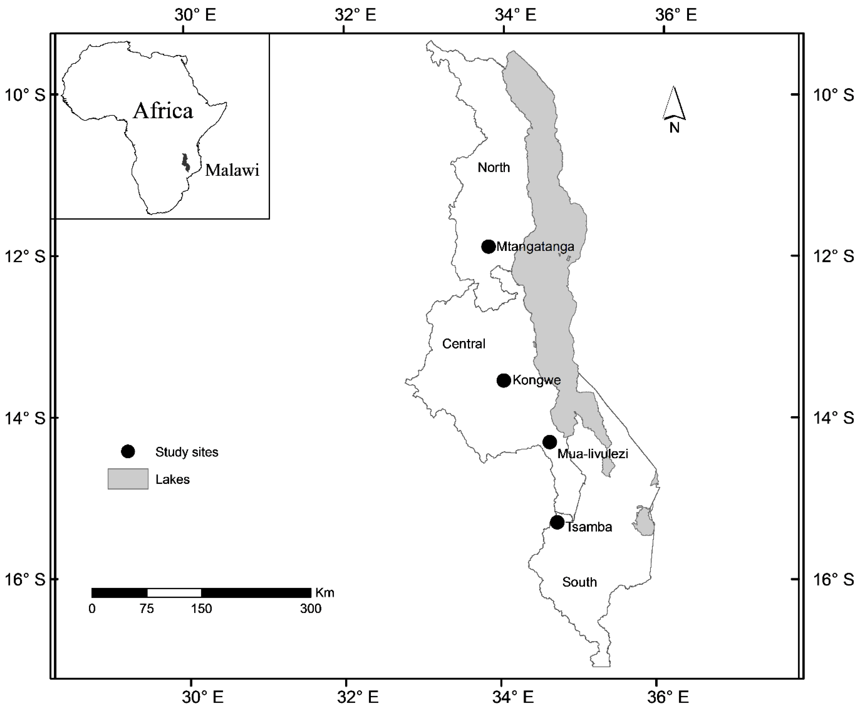
The sample trees for model development were selected from four forest reserves, namely Mtangatanga, Kongwe, Mua-livulezi and Tsamba (Figure 1, Table 1). The selection of sites was based on geographical location, management regime, silvicultural classification, and climatic conditions to capture a wide range of factors influencing tree growth [1].

Figure 1. Map of Malawi showing the location of the study sites.

Figure 1. Map of Malawi showing the location of the study sites.

Table 1. Geographical location, management regime, silvicultural classification and climatic conditions of study sites.

	Mtangatanga	Kongwe	Mua-livulezi	Tsamba
Region	Northern	Central	Central	Southern
District	Mzimba	Dowa	Dedza	Neno
Location	11°56′ S 33°42′ E	13°35′ S 33°55′ E	14°21′ S 34°37′ E	15°21′ S 34°36′ E
Area (ha)	8443	1813	12147	3240
Management regime	Co-management	Government	Co-management	Government
Altitude (m)	1500–1700	1000–1500	400–900	700–1500
Dominant soil type	Humic ferrallitic	Ferruginous	Lithosols	Ferrallitic
Silvicultural classification	Moist Brachystegia	Moist Brachystegia	Dry Brachystegia	Moist Brachystegia
Mean minimum annual temp (°C)	6	6	13	8
Mean maximum annual temp (°C)	29	29	32	28
Total annual rainfall range (mm)	960–1050	960–1050	840–960	1200–1600
Rain period	December–April	November–April	November–April	November–April
Dry months	May–November	May–October	May–October	May–October

Data sources: Rainfall and temperature data (1975–2005) from Ministry of Natural Resources, Energy and Mining, Department of Climate Change and Meteorological Services in Malawi. Soil and silvicultural classification according to Hardcastle [36].

Table 1. Geographical location, management regime, silvicultural classification and climatic conditions of study sites.

	Mtangatanga	Kongwe	Mua-livulezi	Tsamba
Region	Northern	Central	Central	Southern
District	Mzimba	Dowa	Dedza	Neno
Location	11°56′ S 33°42′ E	13°35′ S 33°55′ E	14°21′ S 34°37′ E	15°21′ S 34°36′ E
Area (ha)	8443	1813	12147	3240
Management regime	Co-management	Government	Co-management	Government
Altitude (m)	1500–1700	1000–1500	400–900	700–1500
Dominant soil type	Humic ferrallitic	Ferruginous	Lithosols	Ferrallitic
Silvicultural classification	Moist Brachystegia	Moist Brachystegia	Dry Brachystegia	Moist Brachystegia
Mean minimum annual temp (°C)	6	6	13	8
Mean maximum annual temp (°C)	29	29	32	28
Total annual rainfall range (mm)	960–1050	960–1050	840–960	1200–1600
Rain period	December–April	November–April	November–April	November–April
Dry months	May–November	May–October	May–October	May–October

Data sources: Rainfall and temperature data (1975–2005) from Ministry of Natural Resources, Energy and Mining, Department of Climate Change and Meteorological Services in Malawi. Soil and silvicultural classification according to Hardcastle [36].

2.2. Selection of Sample Trees

We conducted systematic sample plot inventories covering each site to collect information on ranges in tree size and species distribution to guide the selection of sample trees (e.g., [21]). We used circular plots with radius 11.28 m (400 m²). On each plot, we identified all tree species and measured their diameter at breast height (dbh) for all trees with dbh >4 cm. In addition, we sampled three trees within each plot, (one with the smallest, one with a medium and one with the largest dbh), and measured their total height (ht). The inventories covered a total of 221 plots with 70, 30, 71 and 50 plots for Mtangatanga, Kongwe, Mua-livulezi and Tsamba, respectively. The maximum recorded dbh values based on all sample plots in Mtangatanga, Kongwe, Mua-livulezi and Tsamba were 61 cm, 73 cm, 70 cm and 56 cm, respectively, while the number of species identified for the respective sites were 66, 45, 77 and 65. In total, for all the study sites, we identified 139 species. The most frequent species for Mtangatanga, Kongwe, Mua-livulezi and Tsamba were Uapaca kirkiana Müll. Arg., Brachystegia spiciformis Benth., Diplorhynchus condylocarpon (Müll. Arg.) Pichon and Uapaca kirkiana Müll. Arg, respectively.

A total of 74 trees were selected based on the observed dbh and tree species frequency within the sites. We ensured that the trees were selected from all dbh classes observed in the sample plot inventories. In addition, we selected a total of eight trees with larger dbh than those observed in the sample plot inventories to reduce uncertainty when predicting biomass of very large trees. We also selected at least one tree among the eight most frequent species observed in each site. The remaining sample trees were selected randomly among all species. In total, 33 tree species were selected, comprising 10, 10, 12 and 10 different tree species in Mtangatanga, Kongwe, Mua-livulezi and Tsamba, respectively.

Before felling (at a stump height of 30 cm), we recorded scientific and local names, and measured dbh, stump diameter (at 30 cm above ground) and ht (Table 2 and

Table A1. Dataset used for model development.

Site	Scientific Name	Local Name	dbh (cm)	ht (m)	Total Above-Ground Biomass (kg)	Total Below-Ground Biomass (kg)	Use
Mtangatanga	Brachystegia glaucescens Burtt Davy & Hutch.	Musani	6.0	4.4	15.5	17.8	a,b
	Erica benguelensis (Welw. ex Engl.) E.G.H. Oliv.	Msankhanya	9.4	4.0	18.7	6.2	a,b
	Erica benguelensis (Welw. ex Engl.) E.G.H. Oliv.	Msankhanya	13.0	6.0	31.6	N/A	a
	Uapaca kirkiana Müll. Arg.	Msuku	15.0	5.0	73.4	36.8	a,b
	Julbernadia paniculata (Benth.) Troupin	Mtondo	16.5	8.0	106.0	84.2	a,b
	Isoberlinia angolensis (Benth.) Hoyle & Brenan	Kabale	19.4	12.0	266.3	86.5	a,b
	Brachystegia boehmii Taub.	Mombo	20.2	8.0	194.0	N/A	a
	Uapaca kirkiana Müll. Arg.	Msuku	21.0	7.8	175.2	N/A	a
	Brachystegia utilis Burtt Davy & Hutch.	Nzale	23.0	10.0	278.8	N/A	a
	Brachystegia taxifolia Burtt Davy & Hutch.	Mchinji	23.6	10.0	271.8	N/A	a
	Julbernadia paniculata (Benth.) Troupin	Mtondo	27.3	10.0	412.2	N/A	a
	Isoberlinia angolensis (Benth.) Hoyle & Brenan	Kabale	28.6	11.0	445.0	N/A	a
	Brachystegia spiciformis Benth.	Chumbe	36.0	12.0	921.1	N/A	a
	Brachystegia longifolia Benth.	Sanga	36.0	10.8	1173.0	511.1	a,b
	Brachystegia glaucescens Burtt Davy & Hutch.	Musani	48.4	14.5	1847.1	947.1	a,b
	Brachystegia glaucescens Burtt Davy & Hutch.	Musani	50.0	16.0	2160.7	741.5	a,b
	Brachystegia spiciformis Benth.	Chumbe	60.0	18.0	3935.0	1247.0	a,b
	Brachystegia glaucescens Burtt Davy & Hutch.	Musani	68.0	10.5	3233.2	1160.7	a,b
	Brachystegia glaucescens Burtt Davy & Hutch.	Musani	78.0	17.0	4952.1	1567.2	a,b
	Brachystegia glaucescens Burtt Davy & Hutch.	Musani	111.2	18.0	8798.5	3144.9	a,b
Kongwe	Julbernadia paniculata (Benth.) Troupin	Mtondo	9.0	5.0	23.4	11.1	a,b
	Uapaca kirkiana Müll. Arg.	Msuku	10.2	5.0	26.2	N/A	a
	Brachystegia spiciformis Benth.	Chumbe	13.0	6.0	94.9	86.4	a,b
	Brachystegia manga De Wild.	Mpapa/Bovo	17.3	10.0	138.4	85.7	a,b
	Julbernadia paniculata (Benth.) Troupin	Mtondo	21.0	11.0	264.9	154.3	a,b
	Brachystegia utilis Burtt Davy & Hutch.	Nzale	24.5	9.0	368.6	82.1	a,b
	Monotes africanus A. DC.	Mkalakate	27.2	10.0	437.2	N/A	a
	Brachystegia spiciformis Benth.	Chumbe	27.5	9.3	499.9	N/A	a
	Brachystegia boehmii Taub.	Mombo	30.8	14.0	636.5	N/A	a
	Uapaca kirkiana Müll. Arg.	Msuku	34.0	12.0	689.6	201.4	a,b
	Parinari curatellifolia Planch. ex Benth.	Muula	37.3	12.0	839.7	285.7	a,b
	Brachystegia manga De Wild.	Mpapa/Bovo	38.1	17.0	1445.1	N/A	a
	Cussonia arborea Hochst. ex A. Rich.	Mbwabwa	38.4	7.0	346.6	N/A	a
	Brachystegia spiciformis Benth.	Chumbe	38.7	14.0	1298.4	492.7	a,b
	Brachystegia manga De Wild.	Mpapa/Bovo	52.0	22.0	2534.0	N/A	a
	Brachystegia manga De Wild.	Mpapa/Bovo	61.7	17.0	4400.3	1235.3	a,b
	Brachystegia spiciformis Benth.	Chumbe	71.2	18.0	4914.1	1228.4	a,b
	Erythrina abyssinica Lam. ex DC.	Muwale	75.7	12.0	2559.1	N/A	a
Mua-livulezi	Markhamia obtusifolia (Baker) Sprague	Msewa	5.3	5.0	6.3	5.8	a,b
	Combretum apiculatum Sond.	Kakunguni	6.0	3.0	15.0	12.4	a,b
	Bauhinia petersiana Bolle	Mphandula	9.1	5.2	36.5	27.4	a,b
	Bauhinia thonningii Schum.	Msekese	13.0	5.0	61.6	N/A	a
	Diplorhynchus condylocarpon (Müll. Arg.) Pichon	Thombozi	16.2	10.4	84.7	N/A	a
	Annona senegalensis Pers.	Mpoza	17.0	8.0	83.9	45.3	a,b
	Markhamia obtusifolia (Baker) Sprague	Msewa	20.0	9.3	142.8	N/A	a
	Pterocarpus rotundifolius (Sond.) Druce	M’balitsa	22.0	8.5	170.1	N/A	a
	Albizia versicolor Welw. ex Oliv.	Mtangatanga	23.2	10.4	214.6	N/A	a
	Bauhinia petersiana Bolle	Mphandula	27.4	7.9	366.6	N/A	a
	Diplorhynchus condylocarpon (Müll. Arg.) Pichon	Thombozi	31.8	13.0	407.3	169.5	a,b
	Acacia galpinni Burtt Davy	Mgundanjira	37.7	14.0	932.3	232.6	a,b
	Pterocarpus rotundifolius (Sond.) Druce	M'balitsa	42.0	15.0	959.6	N/A	a
	Brachystegia spiciformis Benth.	Chumbe	47.1	15.5	1916.1	349.5	a,b
	Brachystegia bussei Harms	Mtwana	61.0	20.5	3970.5	1337.1	a,b
	Pseudolachnostaylis maprouneifolia Pax	Msolo	61.0	15.6	2994.0	N/A	a
	Brachystegia spiciformis Benth.	Chumbe	69.5	21.0	4580.6	1669.5	a,b
	Brachystegia bussei Harms	Mtwana	81.7	22.0	6758.4	N/A	a
Tsamba	Uapaca kirkiana Müll. Arg.	Msuku	8.4	6.5	18.0	N/A	a
	Brachystegia floribunda Benth.	Tsamba	9.5	9.0	37.5	N/A	a
	Pseudolachnostaylis maprouneifolia Pax	Msolo	12.4	7.0	105.9	N/A	a
	Brachystegia floribunda Benth.	Tsamba	19.9	8.0	287.6	N/A	a
	Parinari excelsa Sabine	Mpembu	21.0	10.0	205.1	86.2	a,b
	Julbernadia globiflora (Benth.) Troupin	Kachumbe	21.0	10.0	223.0	N/A	a
	Brachystegia spiciformis Benth.	Chumbe	21.2	12.0	271.7	210.7	a,b
	Uapaca sansibarica Pax	Msokolowe	22.2	10.0	212.3	110.2	a,b
	Pericorpsis angolensis (Baker) Meeuwen	Muwanga	28.4	8.0	440.2	249.4	a,b
	Uapaca kirkiana Müll. Arg.	Msuku	30.3	11.0	581.9	277.7	a,b
	Pterocarpus angolensis DC.	Mlombwa	31.3	17.0	667.7	218.5	a,b
	Brachystegia utilis Burtt Davy & Hutch.	Nzale	32.0	14.0	867.6	385.8	a,b
	Uapaca sansibarica Pax	Msokolowe	32.0	12.0	445.9	177.3	a,b
	Brachystegia floribunda Benth.	Tsamba	34.5	12.0	683.0	N/A	a
	Julbernadia globiflora (Benth.) Troupin	Kachumbe	37.5	18.0	1014.0	N/A	a
	Faurea speciosa (A. Rich.) Pic.Serm.	Chisese	38.7	16.0	693.7	N/A	a
	Julbernadia globiflora (Benth.) Troupin	Mchenga	67.4	21.0	4591.2	1397.5	a,b
	Brachystegia spiciformis Benth.	Chumbe	75.0	25.0	5866.2	1240.0	a,b

Note: a = aboveground only; a, b = both above-and belowground; N/A = not applicable.

). We used either a calliper or a diameter tape, depending on tree sizes, to measure dbh and stump diameter, while a Suunto hypsometer was used for all ht measurements. These trees have previously been used to develop general volume models for miombo woodlands in Malawi [37].

Table 2. Mean, minimum, maximum and standard deviation (STD) of diameter at breast height (dbh) and total tree height (ht) for sample trees at each site.

Site	No. of Trees	dbh (cm)				ht (m)
		Mean	Min.	Max.	STD	Mean	Min.	Max.	STD
Mtangatanga	20	35.5	6.0	111.2	26.7	10.7	4.0	18.0	4.3
Kongwe	18	34.9	9.0	75.7	19.6	11.7	5.0	22.0	4.7
Tsamba	18	30.2	8.4	75.0	17.5	12.6	6.5	25.0	5.1
Mua-livulezi	18	32.8	5.3	81.7	23.0	11.6	3.0	22.0	5.8
All	74	33.4	5.3	111.2	21.8	11.6	3.0	25.0	4.9

Table 2. Mean, minimum, maximum and standard deviation (STD) of diameter at breast height (dbh) and total tree height (ht) for sample trees at each site.

Site	No. of Trees	dbh (cm)				ht (m)
		Mean	Min.	Max.	STD	Mean	Min.	Max.	STD
Mtangatanga	20	35.5	6.0	111.2	26.7	10.7	4.0	18.0	4.3
Kongwe	18	34.9	9.0	75.7	19.6	11.7	5.0	22.0	4.7
Tsamba	18	30.2	8.4	75.0	17.5	12.6	6.5	25.0	5.1
Mua-livulezi	18	32.8	5.3	81.7	23.0	11.6	3.0	22.0	5.8
All	74	33.4	5.3	111.2	21.8	11.6	3.0	25.0	4.9

2.3. Destructive Sampling

We separated each sample tree into the following aboveground components: merchantable stem (from the stump at 30 cm above ground to the point where the first branches start), branches (all parts of the tree above the defined merchantable stem and up to a minimum diameter of 2.5 cm) and twigs (all branches with a diameter less than 2.5 cm). For small trees not considered suitable for timber production (dbh < 15 cm, in total 14 trees), merchantable stem biomass were allocated to branches (e.g., [37,38]). During the work on destructive sampling most of the trees had already started to shed leaves. We therefore excluded leaves from twigs, and leaves were not included in the models.

To facilitate measurements, stems and branches were crosscut into manageable pieces of approximately 1–2 m in length and then weighed for fresh weight using a mechanical hanging spring balance (0–200 kg). Twigs from each tree were separately bundled and weighed for fresh weight. Three small sub-samples, varying in weight between 0.1 and 1.0 kg, from each of the components (merchantable stem, branches and twigs) were taken from each sample tree and weighed with an electronic balance for fresh weight and finally brought to laboratory for drying. The sub-samples were taken from the biggest, medium and smallest diameter parts of each tree component.

For determination of belowground biomass of the sample trees, our strategy involved root sampling at two levels, namely main roots (roots branching directly from the root crown) and side roots (roots branching from the main roots). The first step in excavation involved clearing the topsoil around the tree base to expose the points at which the roots were branching. We then selected three main roots, i.e., the main roots with the largest, medium and smallest diameters, and recorded their diameters at the points where they joined the root crown. The diameters of all main roots not excavated were recorded at the point where they were joined the root crown. From each of the selected main roots, we selected up to three side roots, i.e., the side roots with the largest, medium and smallest diameters. For each of the selected side roots, we recorded the diameter where they joined the main root. For the remaining side roots, we also recorded the diameters at the branching point from the main root. The selected side and main roots were then fully excavated up to the minimum diameter of 1 cm and then weighed. In cases where the full roots could not be excavated due to obstacles such as rocks, the diameter of the last bit of the root was recorded and we treated the remaining unexcavated part as a side root. An effort was made to ensure that all the main, side and taproots were fully excavated up to the last 1 cm. In total, 38 out of the 41 trees, had taproots. Out of the 38 trees, we were not able to fully excavate the taproots for 16 trees. In such cases, the diameter at the breaking point of the unexcavated taproot was recorded and treated as a side root. On average, trees were dug down to 2.5 m depth. Lastly, we recorded the fresh weight of the root crown for each tree.

For all sample trees, three small sub-samples, varying in weight between 0.1 and 1.0 kg, were taken from each main and side root, and one was taken from the root crown. We obtained the fresh weight of the sub-samples using an electronic balance and brought them to the laboratory for drying.

2.4. Laboratory Analyses and Determination of Biomass Dry Weight

All sub-samples, from both above- and belowground, for each tree were dried in an oven in a laboratory at a temperature of 80 °C until a constant weight was achieved (constant weight was observed in 2–3 days). We then recorded dry weights of the individual sub-samples. Subsequently, we used the sub-sample dry and fresh weights to determine the tree- and section specific dry to fresh weight ratios (DF-ratios) (see

Table A2. DF-ratio for merchantable stem, branches, twigs, roots, and root crown in the four study sites.

Site	Aboveground										Belowground
	No. of Trees	Merchantable Stem			Branches			Twigs			No. of Trees	Roots			Root crown
		Mean	Min	Max	Mean	Min	Max	Mean	Min	Max		Mean	Min	Max	Mean	Min	Max
Mtangatanga	20	0.61	0.48	0.77	0.57	0.44	0.73	0.51	0.30	0.66	12	0.58	0.46	0.69	0.59	0.53	0.67
Kongwe	18	0.56	0.36	0.71	0.54	0.35	0.65	0.52	0.37	0.65	10	0.58	0.48	0.72	0.57	0.39	0.67
Mua-livulezi	18	0.60	0.54	0.69	0.61	0.54	0.67	0.56	0.44	0.66	9	0.60	0.49	0.70	0.59	0.46	0.68
Tsamba	18	0.59	0.45	0.70	0.58	0.45	0.67	0.53	0.38	0.65	10	0.52	0.45	0.63	0.57	0.51	0.61
All	74	0.59	0.36	0.77	0.58	0.35	0.73	0.53	0.30	0.66	41	0.57	0.45	0.73	0.58	0.39	0.68

Note: The number of sample trees for Kongwe for the twigs section is 16 instead of 18 because two trees did not have twigs.

).

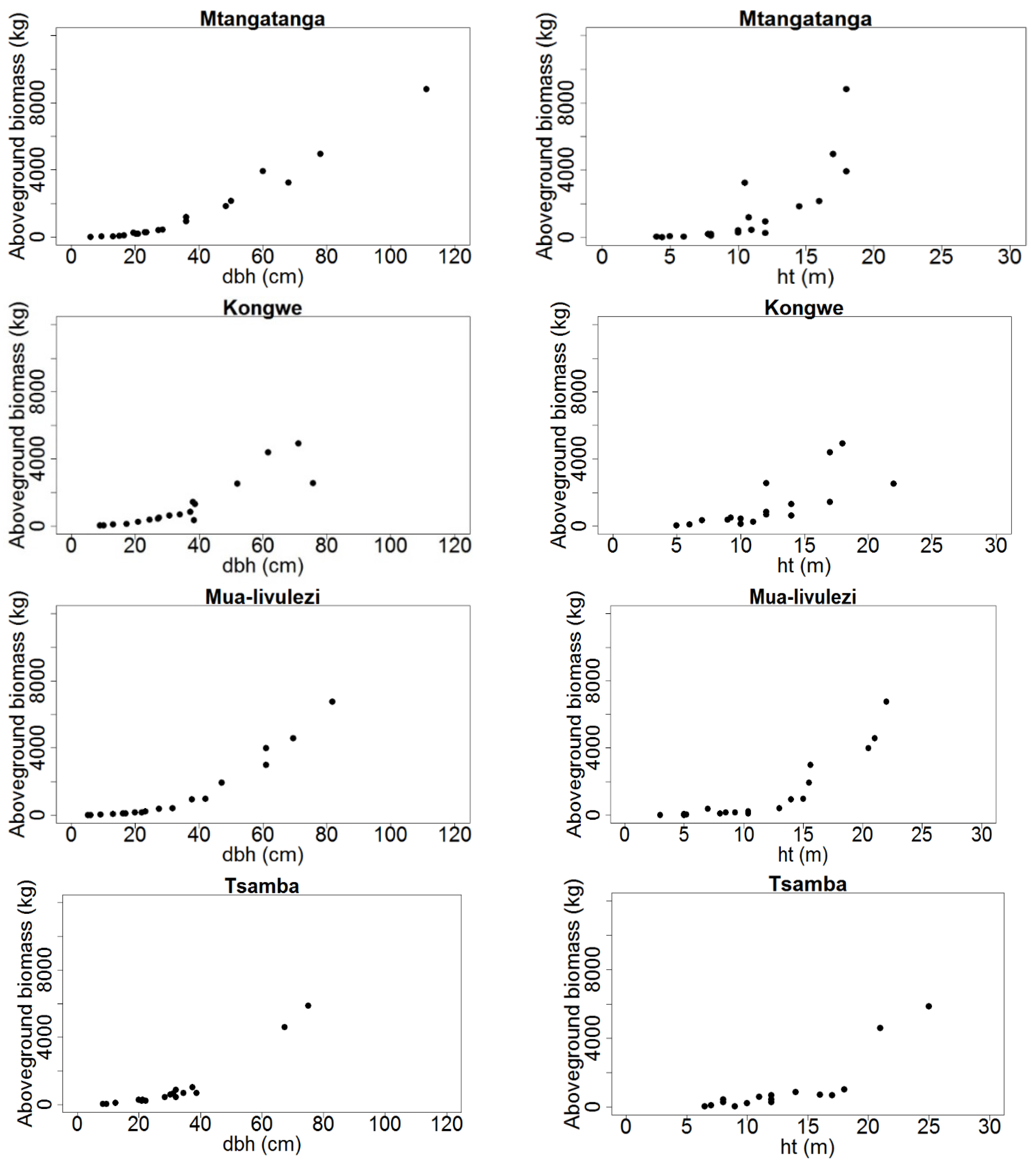
We then calculated the dry weight of each section as a product of tree- and section specific DF-ratios and the fresh weights of the respective trees and tree sections. Subsequently, we computed the total aboveground dry weight by summing the dry weights of the merchantable stem, branches and twigs of each tree (Figure 2, Table A1).

Figure 2. Total aboveground tree biomass (kg dry weight) distribution over dbh (cm) and ht (m) for Mtangatanga, Kongwe, Mua-livulezi and Tsamba and forest reserves.

Figure 2. Total aboveground tree biomass (kg dry weight) distribution over dbh (cm) and ht (m) for Mtangatanga, Kongwe, Mua-livulezi and Tsamba and forest reserves.

To determine the total belowground dry weights of the excavated parts of the trees we first converted all the fresh weights from the different sections to dry weight biomass by multiplying the tree- and section specific DF-ratios and their respective fresh weights. We then developed a general (combining data from all sites) side root model by regressing the dry weight biomass of the fully excavated side roots and their diameters (cm). We assumed the relationship between side root biomass and root diameter (similarly for main roots, see below) to exhibit a power-law relationship described as:

$$\mathrm{B}=\mathrm{a} \times {\mathrm{d}}^{\mathrm{b}}$$

(1)

where B = dry weight biomass of a side root or main root (kg); d = diameter (cm) of a side or main root at the point it is joining the main root or the root crown, respectively; a and b are parameter estimates. The following side root model was developed:

$$\mathrm{B}= 0.198102\times {\mathrm{d}}^{1.656968}, \text{Pseudo}-R^2=0.67, \text{MPE}\%= -2.0$$

(2)

where

$$\text{Pseudo}-R^2= 1- \left(\frac{\text{SSR}}{\text{CSST}}\right)$$

(3)

SSR is the sum of squared residuals and CSST is the corrected total sum of squares. The mean prediction error (MPE), and the relative mean prediction error (MPE%) is calculated as

$$\text{MPE}= {{\displaystyle \sum }}_{i=1}^n\frac{\left(y_i-{\widehat{y}}_i\right)}{n}, \text{MPE}\%= \frac{\text{MPE}}{\overline{y}} \times 100$$

(4)

where $y_i$ is the observed biomass of tree i, ${\widehat{y}}_i$is the predicted biomass of tree i and $\overline{y}$ is the mean observed biomass. Both MPE and MPE% are based on leave-one-out-cross validation. The MPE% value for the side root model was not significantly different from zero indicating appropriate model performance.

The side root model was used to predict the dry weight biomass of all the side roots that were not excavated for the main sample root. The total dry weight of all side roots for each main sample root was then determined by summing dry weights of the excavated side roots and predicted dry weights of unexcavated side roots. Finally the complete dry weight of the sample main root was determined by summing the total dry weights of all side roots and the excavated parts of the main root. The following main root model was then developed and applied to predict the dry weights of main roots not excavated;

$$\mathrm{B}= 0.063132\times {\mathrm{d}}^{2.174388}, \text{Pseudo}-R^2=0.79, \text{MPE}\%= -0.4$$

(5)

The MPE% value for the main root model was not significantly different from zero indicating appropriate model performance. To determine the dry weight of unexcavated parts of the taproots (16 trees), we applied the general side root model.

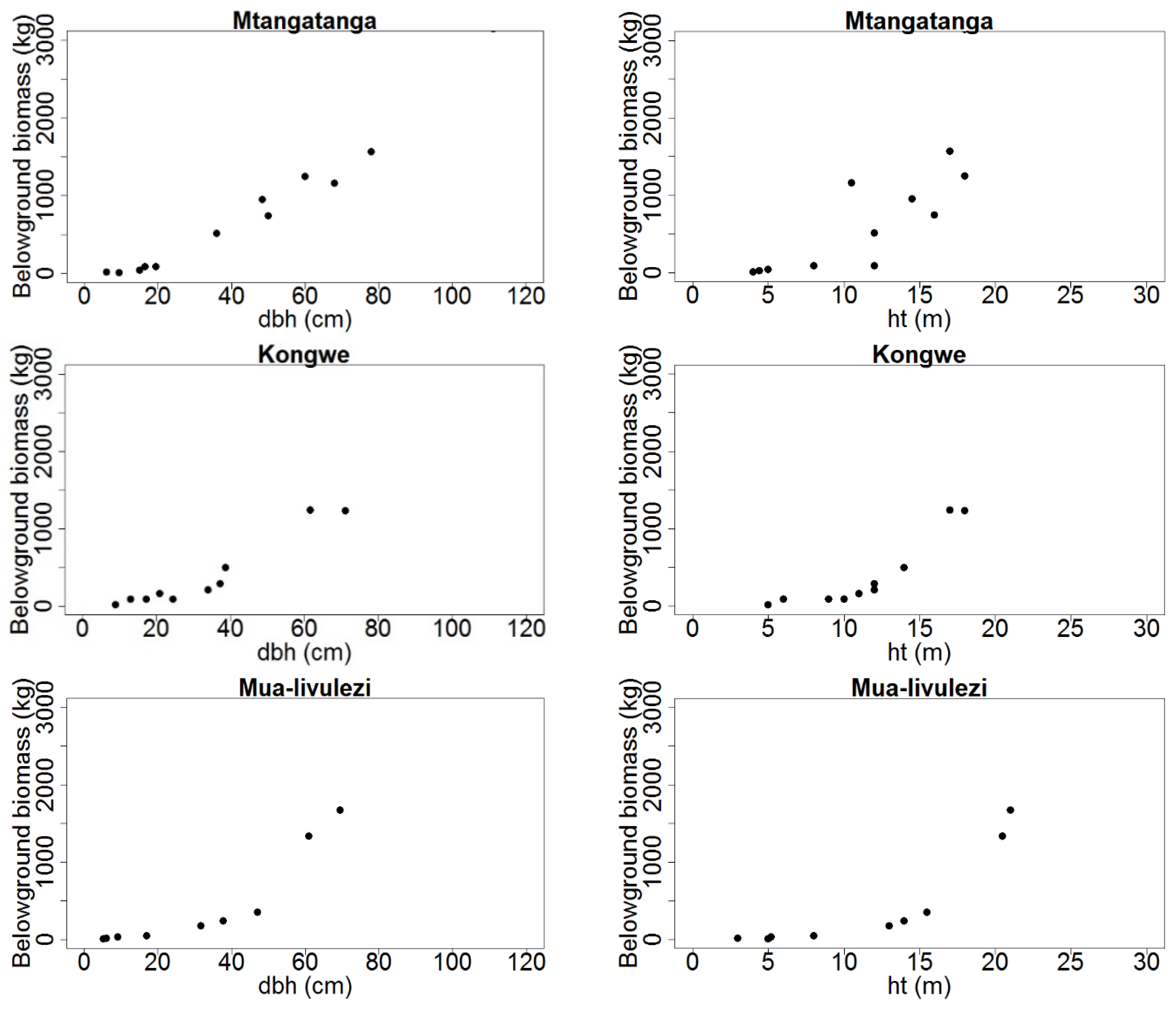
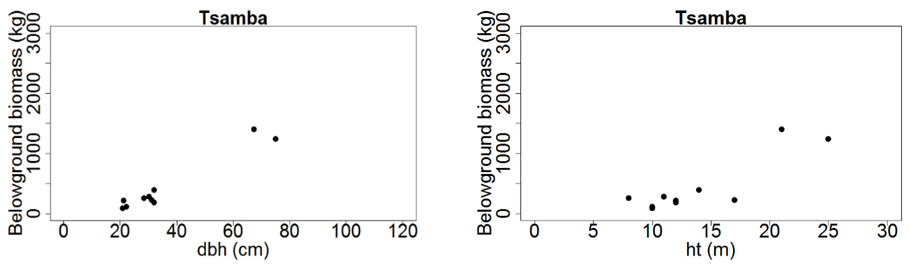
Total belowground dry weight biomass for each tree was finally determined by adding the dry weights of all excavated and unexcavated main roots, dry weight of the taproot, and the dry weight of the root crown (Figure 3, Table A1).

Figure 3. Total belowground tree biomass (kg dry weight) distribution over dbh (cm) and ht (m) for Mtangatanga, Kongwe, Mua-livulezi and Tsamba and forest reserves.

Figure 3. Total belowground tree biomass (kg dry weight) distribution over dbh (cm) and ht (m) for Mtangatanga, Kongwe, Mua-livulezi and Tsamba and forest reserves.

2.5. Model Development and Evaluation

Before fitting the models, we assessed the basic diagnostic plots of biomass over dbh and ht. As expected, the plots indicated non-linear patterns in the relationships between biomass and dbh and ht (Figure 2 and Figure 3). Since wood specific gravity ($\mathsf{\rho }$) is considered as an important factor for explaining variation in biomass (e.g., [39]), we included this variable in the models. We therefore tested the following models:

$$\text{Model} 1: \mathrm{B}=\mathrm{a}\times {\text{dbh}}^{\mathrm{b}}$$

(6)

$$\text{Model} 2: \mathrm{B}=\mathrm{a}\times {\text{dbh}}^{\mathrm{b}}\times {\text{ht}}^{\mathrm{c}}$$

(7)

$$\text{Model} 3: \mathrm{B}=\mathrm{a}\times {\text{dbh}}^{\mathrm{b}}\times {\mathsf{\rho }}^{\mathrm{c}}$$

(8)

$$\text{Model} 4: \mathrm{B}=\mathrm{a}\times {\text{dbh}}^{\mathrm{b}}\times {\text{ht}}^{\mathrm{c}}\times {\mathsf{\rho }}^{\mathrm{d}}$$

(9)

where B is biomass (kg), dbh is diameter at breast height (cm), ht is total tree height (m) and $\mathsf{\rho }$ is the species-specific mean wood specific gravity (g/cm³) extracted from the global wood density database [40,41] and a, b, c and d are parameter estimates.

Since the data was collected from different study sites in different geographical regions and silvicultural zones across Malawi, we anticipated that individual tree attributes would be different depending on site. We therefore initially fitted mixed effects models, with site as a random effect, to the side root, main root and total belowground and aboveground biomass datasets using PROC NLMIXED of SAS 9.4 [42]. This procedure fits nonlinear mixed models, that is, models in which both fixed and random effects enter nonlinearly. PROC NLMIXED fits nonlinear mixed models by maximizing an approximation to the likelihood integrated over the random effects using the maximum likelihood estimation method.

These mixed effects models were compared with weighted nonlinear regression models fitted using PROC MODEL in SAS 9.4 [42]. This procedure fits models in which the relationships among the variables comprise a system of one or more nonlinear equations using the full information maximum likelihood (FIML) estimation method.

For each model derived from the two procedures, i.e., mixed effects and weighted regression, we computed Akaike Information Criterion (AIC) values [43]. AIC measures the model goodness-of-fit whilst correcting for model complexity. We used the AIC values to compare mixed effects models with the weighted regression nonlinear models. The results showed that, in all cases, weighted regression models produced lower AIC values relative to mixed effects models. We thus decided to develop our final models based on weighted regression.

Model efficiency and performance were assessed based on results from a leave-one-out cross validation procedure [44]. This splits the dataset of n observations into two parts, namely, a validation dataset and a training dataset. The validation dataset comprises a single observation (x₁, y₁) and the training dataset comprises the remaining {(x₂, y₂),….., (x_n, y_n)} observations. The model is fitted on the n-1 observations in the training dataset and a prediction $\widehat{y }$ is made for a single observation in the validation dataset, using its value x₁. Since (x₁, y₁) was not used in the fitting process, the square error (SE) = (y₁−$\widehat{y}$)² provides an estimate of the test error. This procedure is repeated n times, thus producing n test errors, SE₁…….SE_n. The leave-one-out-cross validation estimate for the test error is the mean of these n test error estimates (MSE).

The cross validation results were then used to calculate the root mean square error (RMSE) as follows;

$$\text{RMSE}=\sqrt{\text{MSE}}$$

(10)

$$\text{RMSE }(\%)=\frac{\text{RMSE}}{\overline{\mathrm{y}}}\times 100$$

(11)

where $\overline{\mathrm{y}}$ is the mean observed biomass and RMSE (%) is the relative Root Mean Square Error.

Model comparison was based on AIC values. Models with insignificant parameter estimates were not considered irrespective of AIC values. For all the models, we presented pseudo-R², RMSE, RMSE (%), covariance matrix for the parameter estimates, and the MPE and MPE% values based on leave-one-out cross validation. Student t-tests were conducted to determine whether the MPE values were significantly different from zero.

In addition, we tested a number of previously developed biomass models (Table 3) on our data. This included models developed for miombo woodlands in neighbouring countries, i.e., Ryan et al. [4] in Mozambique, Mugasha et al. [21] in Tanzania and Chidumayo [18] in Zambia, and the pan-tropical model developed by Chave et al. [39]. MPE values were computed, and student t-tests were applied to determine whether the MPE values were significantly different from zero.

For a graphical display of the behaviour of models with ht as independent variable, i.e., Mugasha et al. [21] and Chave et al. [39] (see Table 3), we applied a height-diameter model developed from our sample trees:

$$\text{ht}=1.3+\exp 3.787685-6.62809 \times {\text{dbh}}^{-0.45222}$$

(12)

Furthermore, when applying Chave et al. [39], we extracted $\mathsf{\rho }$ values from the global wood density database [40,41] and subsequently calculated a mean $\mathsf{\rho }$ value, which was then used for the graphical display of this model.

Table 3. Number of sites, sample trees and dbh ranges (cm) of previously developed models tested on our data.

Tree Section	Author	Model	No. of Sites	No. of Trees	dbh Range (cm)	Species
Above-Ground	Mugasha et al. [21]	$\mathrm{B}=0.1027\times {\text{dbh}}^{2.4798}$	4	167	1.1–110	60
	Mugasha et al. [21]	$\mathrm{B}=0.0763\times {\text{dbh}}^{2.2046}\times {\text{ht}}^{0.4918}$	4	167	1.1–110	60
	Ryan et al. [4] a	$\mathrm{C}=-3.629+2.601\times \log \left(\text{dbh}\right)$	1	29	5–73	6
	Chidumayo [18]	$\mathrm{B}=-2.5265+2.5553\times \log \left(\text{dbh}\right)$	1	113	2–39	19
	Chave et al. [39] b	$\mathrm{B}=0.0673\times {\left(\mathsf{\rho }\times {\text{dbh}}^2\times \text{ht}\right)}^{0.976}$	58	4004	5–180	Unclear
Below-Ground	Mugasha et al. [21]	$\mathrm{B}=0.2113\times {\text{dbh}}^{1.9838}$	4	80	3.3–95	60
	Mugasha et al. [21]	$\mathrm{B}=0.1766\times {\text{dbh}}^{1.7844}\times {\text{ht}}^{0.3434}$	4	80	3.3–95	60
	Ryan et al. [4] a	$\mathrm{C}=-3.370+2.262\times \log \left(\text{dbh}\right)$	1	23	5–72	6
	Chidumayo [18]	$\mathrm{B}=-1.9439+2.1712\times \log \left(\text{dbh}\right)$	1	12	4–35	19

^a Carbon converted to biomass as $\mathrm{B}=\left(\raisebox{1ex}{$\mathrm{C}$}\!\left/ \!\raisebox{-1ex}{$47$}\right.\right) \times 100$; ^b $\mathsf{\rho }$ (g/cm³) is the species-specific mean wood specific gravity (g/cm³) extracted from the global wood density database [40,41].

Table 3. Number of sites, sample trees and dbh ranges (cm) of previously developed models tested on our data.

Tree Section	Author	Model	No. of Sites	No. of Trees	dbh Range (cm)	Species
Above-Ground	Mugasha et al. [21]	$\mathrm{B}=0.1027\times {\text{dbh}}^{2.4798}$	4	167	1.1–110	60
	Mugasha et al. [21]	$\mathrm{B}=0.0763\times {\text{dbh}}^{2.2046}\times {\text{ht}}^{0.4918}$	4	167	1.1–110	60
	Ryan et al. [4] a	$\mathrm{C}=-3.629+2.601\times \log \left(\text{dbh}\right)$	1	29	5–73	6
	Chidumayo [18]	$\mathrm{B}=-2.5265+2.5553\times \log \left(\text{dbh}\right)$	1	113	2–39	19
	Chave et al. [39] b	$\mathrm{B}=0.0673\times {\left(\mathsf{\rho }\times {\text{dbh}}^2\times \text{ht}\right)}^{0.976}$	58	4004	5–180	Unclear
Below-Ground	Mugasha et al. [21]	$\mathrm{B}=0.2113\times {\text{dbh}}^{1.9838}$	4	80	3.3–95	60
	Mugasha et al. [21]	$\mathrm{B}=0.1766\times {\text{dbh}}^{1.7844}\times {\text{ht}}^{0.3434}$	4	80	3.3–95	60
	Ryan et al. [4] a	$\mathrm{C}=-3.370+2.262\times \log \left(\text{dbh}\right)$	1	23	5–72	6
	Chidumayo [18]	$\mathrm{B}=-1.9439+2.1712\times \log \left(\text{dbh}\right)$	1	12	4–35	19

^a Carbon converted to biomass as $\mathrm{B}=\left(\raisebox{1ex}{$\mathrm{C}$}\!\left/ \!\raisebox{-1ex}{$47$}\right.\right) \times 100$; ^b $\mathsf{\rho }$ (g/cm³) is the species-specific mean wood specific gravity (g/cm³) extracted from the global wood density database [40,41].

3. Results

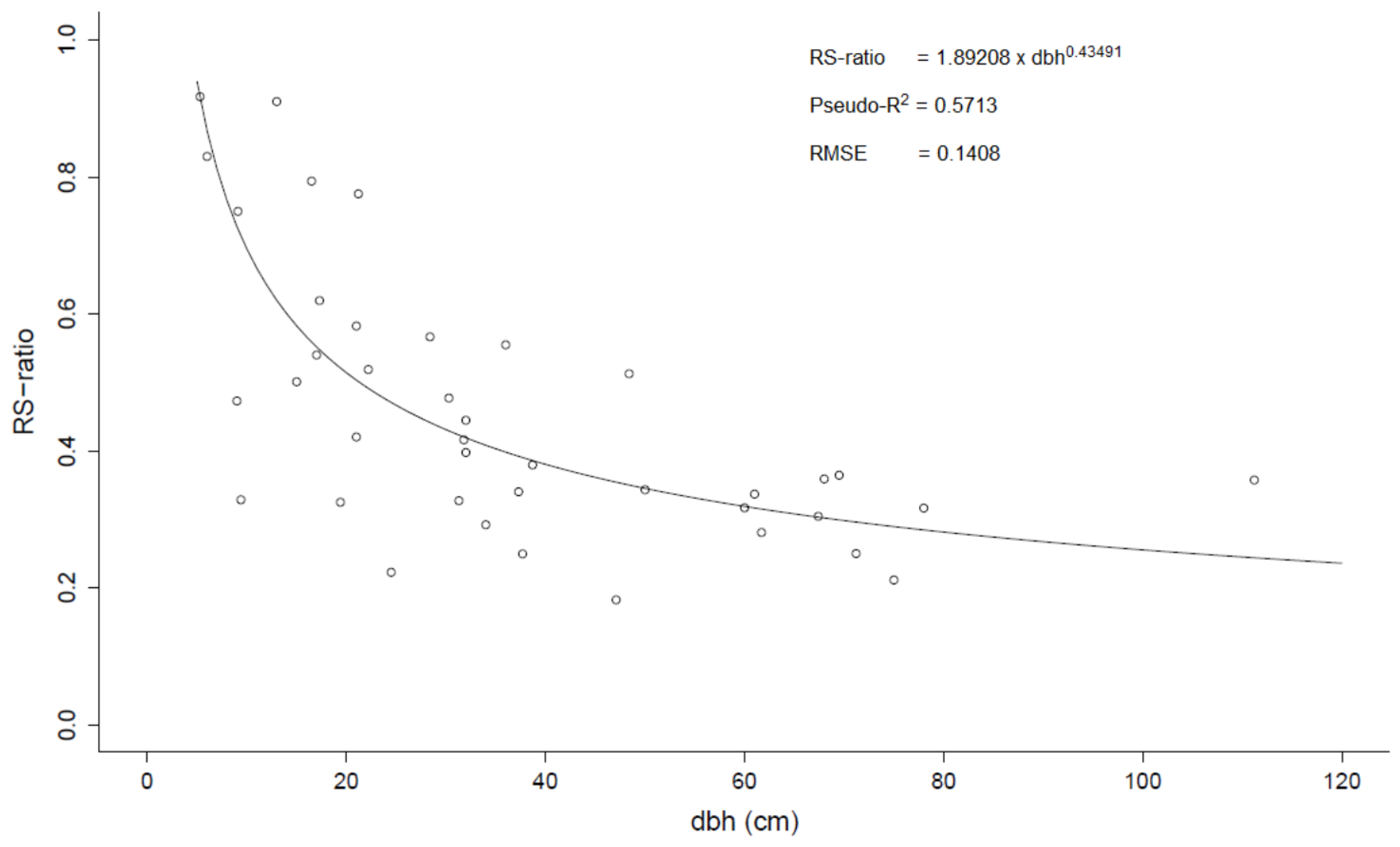
The mean RS-ratio of the 41 trees sampled both above- and belowground was 0.47 (Table 4). No significant differences in RS-ratios were found between sites (p = 0.8684, F = 0.2400). The RS-ratio decreased nonlinearly with increasing dbh (Figure 4).

Table 4. Mean, standard deviation (STD) and range of root to shoot ratios (RS-ratio) over sites.

Site	No. of Trees	Mean	Min	Max	STD
Mtangatanga	12	0.49	0.32	1.15	0.25
Kongwe	10	0.44	0.22	0.91	0.22
Mua-livulezi	9	0.51	0.27	0.92	0.27
Tsamba	10	0.44	0.21	0.78	0.16
All	41	0.47	0.18	1.15	0.22

Table 4. Mean, standard deviation (STD) and range of root to shoot ratios (RS-ratio) over sites.

Site	No. of Trees	Mean	Min	Max	STD
Mtangatanga	12	0.49	0.32	1.15	0.25
Kongwe	10	0.44	0.22	0.91	0.22
Mua-livulezi	9	0.51	0.27	0.92	0.27
Tsamba	10	0.44	0.21	0.78	0.16
All	41	0.47	0.18	1.15	0.22

Figure 4. Root to shoot ratio (RS-ratio) vs. diameter at breast height (dbh). The dots represent observations for individual trees and the line represents the fitted nonlinear model.

Figure 4. Root to shoot ratio (RS-ratio) vs. diameter at breast height (dbh). The dots represent observations for individual trees and the line represents the fitted nonlinear model.

For aboveground biomass, all models, except Model 4, had significant parameter estimates and appropriate performance criteria, i.e., none of the models had MPE% values significantly different from zero (p > 0.05) (Table 5). Among these models, Model 2 with dbh and ht as independent variables had the smallest AIC value. The pseudo-R² values for all models ranged from 0.93 to 0.97. For belowground biomass, Model 1 was the only one where all parameter estimates were significant. Covariance matrices for all models with significant parameter estimates in Table 5 are shown in

Table A3. Covariance matrices of all valid above- and belowground models.

Component	Model No.	Model	Variable	Covariance Matrix
Belowground	1	0.284615 × dbh1.992658		intercept	dbh
			intercept	0.01184
			dbh	−0.01018	0.00882
Aboveground	1	0.21691 × dbh2.318391		intercept	dbh
			intercept	0.00251
			dbh	−0.00263	0.00278
	2	0.103685 × dbh1.921719 × ht0.844561		intercept	dbh	ht
			intercept	0.00058
			dbh	−0.00045	0.00166
			ht	−0.00129	−0.00094	0.00580
	3	0.290457 × dbh2.283998 × $\mathsf{\rho }$0.443619		intercept	dbh	$\mathsf{\rho }$
			intercept	0.00592
			dbh	−0.00422	0.00305
			$\mathsf{\rho }$	0.00557	−0.00346	0.01364

.

Among the models with significant parameter estimates for twigs, branches and merchantable stem biomass (Table 6), Models 1, 2 and 2, respectively, provided the smallest AIC values. The pseudo-R² values for the twigs, branches and merchantable stem models with significant parameter estimates were 0.82, 0.91–0.92 and 0.77–0.88, respectively.

We further evaluated the above- and belowground biomass models over sites and dbh classes (Table 7). None of the tested models produced MPE values significantly different from zero (p > 0.05) overall or for any site. However, a significant MPE was observed for dbh class 0–20 cm for Model 3. For the aboveground biomass models, MPE% values ranged from 0.4% to 15.1% while for the belowground biomass model, the MPE% values ranged from 2.1% to 3.9%.

Finally, we tested previously developed models (Table 3) on our dataset (Table 8). The MPE% when applying the aboveground biomass models developed by Mugasha et al. [21], Ryan et al. [4], Chidumayo [18] and Chave et al. [39] ranged from 2.8 to 30.8 (under prediction). The above- and belowground biomass models developed by Chidumayo [18] generally produced the lowest MPE% values, i.e., 2.8% and −4.7%, respectively. 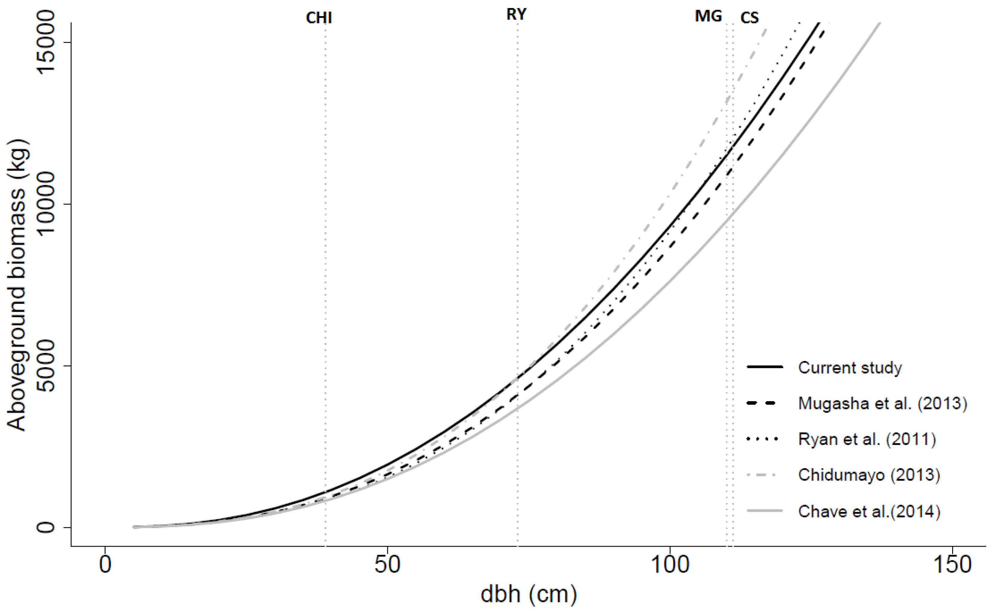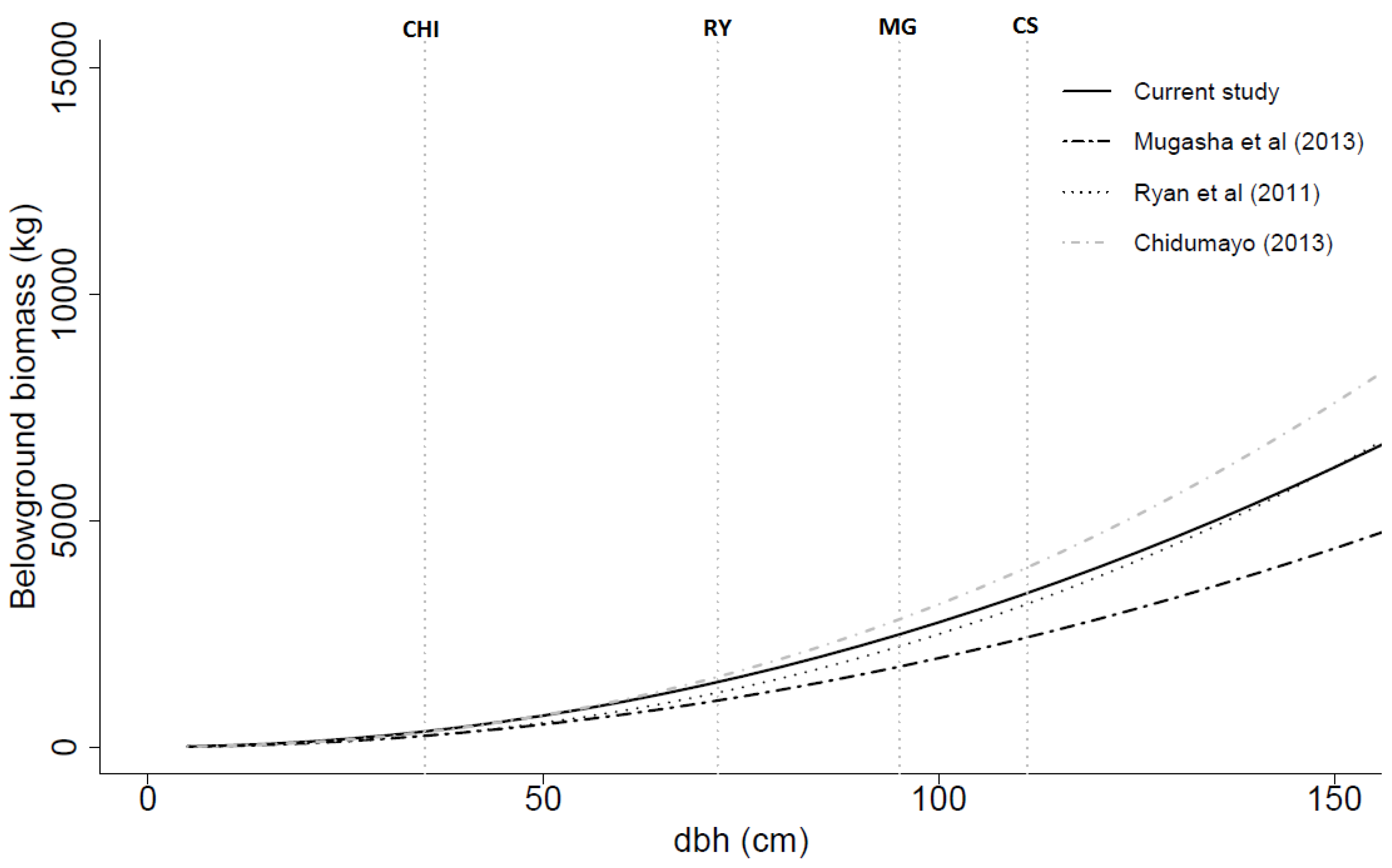Figure 5 and Figure 6 display above- and belowground biomass over dbh for some of the models developed in the current study and some from the previous studies.

Table 5. Model parameters and performance criteria of above- and belowground biomass models.

Component	Model No.	No. of Trees	Model	Pseudo-R2	RMSE		MPE		AIC
					(kg)	(%)	(kg)	(%)
Aboveground	1	74	$0.21691\times {\text{dbh}}^{2.318391}$	0.93	751.2	60.6	−22.2	−1.8	981.89
	2	74	$0.103685 \times db{h}^{1.921719}\times h{t}^{0.844561}$	0.97	426.6	34.4	−19.8	−1.6	954.27
	3	74	$0.290457\times {\text{dbh}}^{2.283998}\times {\mathsf{\rho }}^{0.443619}$	0.94	923.1	74.5	−53.2	−4.3	977.05
	4	74	$0.129899\times {\text{dbh}}^{1.90203}\times {\text{ht}}^{0.828647}\times {\mathsf{\rho }}^{0.296271\text{NS}}$	0.97	542.1	43.7	−37.1	−3.0	952.35
Belowground	1	41	$0.284615\times db{h}^{1.992658}$	0.94	161.7	30.7	−4.8	−0.9	481.23
	2	41	$0.224132\times {\text{dbh}}^{1.899061}\times {\text{ht}}^{0.222554\text{NS}}$	0.94	169.7	32.2	−7.4	−1.4	481.73
	3	41	$0.415451\times {\text{dbh}}^{1.933905}\times {\mathsf{\rho }}^{0.465663\text{NS}}$	0.94	175.4	33.3	−5.0	−1.0	481.74
	4	41	$0.350488\times {\text{dbh}}^{1.732452}\times {\text{ht}}^{0.395127\text{NS}}\times {\mathsf{\rho }}^{0.836154\text{NS}}$	0.94	170.2	32.3	−6.5	−1.2	479.66

^NS Parameter estimate not significant (p > 0.05). Note: biomass in kg, dbh in cm, ht in m, and $\mathsf{\rho }$ in g/cm³, Bold: best model according to AIC (Akaike Information Criterion (AIC)).

Table 5. Model parameters and performance criteria of above- and belowground biomass models.

Component	Model No.	No. of Trees	Model	Pseudo-R2	RMSE		MPE		AIC
					(kg)	(%)	(kg)	(%)
Aboveground	1	74	$0.21691\times {\text{dbh}}^{2.318391}$	0.93	751.2	60.6	−22.2	−1.8	981.89
	2	74	$0.103685 \times db{h}^{1.921719}\times h{t}^{0.844561}$	0.97	426.6	34.4	−19.8	−1.6	954.27
	3	74	$0.290457\times {\text{dbh}}^{2.283998}\times {\mathsf{\rho }}^{0.443619}$	0.94	923.1	74.5	−53.2	−4.3	977.05
	4	74	$0.129899\times {\text{dbh}}^{1.90203}\times {\text{ht}}^{0.828647}\times {\mathsf{\rho }}^{0.296271\text{NS}}$	0.97	542.1	43.7	−37.1	−3.0	952.35
Belowground	1	41	$0.284615\times db{h}^{1.992658}$	0.94	161.7	30.7	−4.8	−0.9	481.23
	2	41	$0.224132\times {\text{dbh}}^{1.899061}\times {\text{ht}}^{0.222554\text{NS}}$	0.94	169.7	32.2	−7.4	−1.4	481.73
	3	41	$0.415451\times {\text{dbh}}^{1.933905}\times {\mathsf{\rho }}^{0.465663\text{NS}}$	0.94	175.4	33.3	−5.0	−1.0	481.74
	4	41	$0.350488\times {\text{dbh}}^{1.732452}\times {\text{ht}}^{0.395127\text{NS}}\times {\mathsf{\rho }}^{0.836154\text{NS}}$	0.94	170.2	32.3	−6.5	−1.2	479.66

^NS Parameter estimate not significant (p > 0.05). Note: biomass in kg, dbh in cm, ht in m, and $\mathsf{\rho }$ in g/cm³, Bold: best model according to AIC (Akaike Information Criterion (AIC)).

Table 6. Model and performance criteria for twigs, branches and merchantable stem biomass models.

Component	Model No.	No. of Trees	Model	Pseudo-R2	RMSE		MPE		AIC
					(kg)	(%)	(kg)	(%)
Twigs	1	72	$0.07239 \times db{h}^{1.858897}$	0.82	39.3	62.5	−0.8	−1.2	602.84
	2	72	$0.070224\times {\mathrm{dbh}}^{1.598204}\times {\mathrm{ht}}^{0.384139\text{NS}}$	0.84	37.8	60.1	−1.1	−1.7	634.09
	3	72	$0.130116\times {\text{dbh}}^{1.764995}\times {\mathsf{\rho }}^{0.687581\text{NS}}$	0.83	44.3	70.4	−1.4	−2.2	616.35
	4	72	${0.109969}^{\text{NS}}\times {\text{dbh}}^{1.446488}\times {\text{ht}}^{0.549901}\times {\mathsf{\rho }}^{0.951968}$	0.83	40.2	63.9	−1.5	−2.4	631.63
Branches	1	74	$0.137316\times {\text{dbh}}^{2.328104}$	0.91	659.8	80.9	−25.4	−3.1	973.58
	2	74	$0.051157 \times db{h}^{2.161115}\times h{t}^{0.598879}$	0.92	565.2	69.3	−22.6	−2.8	933.50
	3	74	$0.123375\times {\text{dbh}}^{2.379626}\times {\mathsf{\rho }}^{0.30643\text{NS}}$	0.91	789.0	96.8	−47.5	−5.8	946.79
	4	74	$0.059792\times {\text{dbh}}^{2.150762}\times {\text{ht}}^{0.582627}\times {\mathsf{\rho }}^{0.20053\text{NS}}$	0.92	692.2	84.9	−39.3	−4.8	934.74
Merchantable	1	60	$0.145576\times {\text{dbh}}^{2.116265}$	0.77	299.9	66.9	−1.2	−0.3	773.89
Stem	2	60	$0.030811\times db{h}^{1.572422}\times h{t}^{1.345696}$	0.88	249.9	55.8	5.3	1.2	737.16
	3	60	$0.221213\times {\text{dbh}}^{2.059249}\times {\mathsf{\rho }}^{0.544483}$	0.79	330.2	73.7	−13.9	−3.1	772.48
	4	60	$0.039194\times {\text{dbh}}^{1.554911}\times {\text{ht}}^{1.329832}\times {\mathsf{\rho }}^{0.36722\text{NS}}$	0.88	256.2	57.2	2.6	0.6	737.75

^NS Parameter estimate not significant (p > 0.05). Note: biomass in kg, dbh in cm, ht in m, and $\mathsf{\rho }$ in g/cm³. Bold: best model according to AIC.

Table 6. Model and performance criteria for twigs, branches and merchantable stem biomass models.

Component	Model No.	No. of Trees	Model	Pseudo-R2	RMSE		MPE		AIC
					(kg)	(%)	(kg)	(%)
Twigs	1	72	$0.07239 \times db{h}^{1.858897}$	0.82	39.3	62.5	−0.8	−1.2	602.84
	2	72	$0.070224\times {\mathrm{dbh}}^{1.598204}\times {\mathrm{ht}}^{0.384139\text{NS}}$	0.84	37.8	60.1	−1.1	−1.7	634.09
	3	72	$0.130116\times {\text{dbh}}^{1.764995}\times {\mathsf{\rho }}^{0.687581\text{NS}}$	0.83	44.3	70.4	−1.4	−2.2	616.35
	4	72	${0.109969}^{\text{NS}}\times {\text{dbh}}^{1.446488}\times {\text{ht}}^{0.549901}\times {\mathsf{\rho }}^{0.951968}$	0.83	40.2	63.9	−1.5	−2.4	631.63
Branches	1	74	$0.137316\times {\text{dbh}}^{2.328104}$	0.91	659.8	80.9	−25.4	−3.1	973.58
	2	74	$0.051157 \times db{h}^{2.161115}\times h{t}^{0.598879}$	0.92	565.2	69.3	−22.6	−2.8	933.50
	3	74	$0.123375\times {\text{dbh}}^{2.379626}\times {\mathsf{\rho }}^{0.30643\text{NS}}$	0.91	789.0	96.8	−47.5	−5.8	946.79
	4	74	$0.059792\times {\text{dbh}}^{2.150762}\times {\text{ht}}^{0.582627}\times {\mathsf{\rho }}^{0.20053\text{NS}}$	0.92	692.2	84.9	−39.3	−4.8	934.74
Merchantable	1	60	$0.145576\times {\text{dbh}}^{2.116265}$	0.77	299.9	66.9	−1.2	−0.3	773.89
Stem	2	60	$0.030811\times db{h}^{1.572422}\times h{t}^{1.345696}$	0.88	249.9	55.8	5.3	1.2	737.16
	3	60	$0.221213\times {\text{dbh}}^{2.059249}\times {\mathsf{\rho }}^{0.544483}$	0.79	330.2	73.7	−13.9	−3.1	772.48
	4	60	$0.039194\times {\text{dbh}}^{1.554911}\times {\text{ht}}^{1.329832}\times {\mathsf{\rho }}^{0.36722\text{NS}}$	0.88	256.2	57.2	2.6	0.6	737.75

^NS Parameter estimate not significant (p > 0.05). Note: biomass in kg, dbh in cm, ht in m, and $\mathsf{\rho }$ in g/cm³. Bold: best model according to AIC.

Table 7. Mean prediction errors (MPE) of the models over study sites and dbh classes.

Component	Model No.	Variable		No. of Trees	Observed	Predicted	MPE
					(kg)	(kg)	(kg)	(%)
Aboveground	1	Site	Mtangatanga	20	1465.5	1606.2	−140.8	−9.6
			Kongwe	18	1195.4	1200.6	−5.2	−0.4
			Mua-livulezi	18	1316.7	1231.5	85.3	6.5
			Tsamba	18	956.3	882.4	73.8	7.7
		dbh class	0–20	21	79.7	93.4	−13.6	−17.1
		(cm)	21–40	35	545.6	584.1	−38.5	−7.1
			41–60	6	2225.4	1911.6	313.9	14.1
			>60	12	4801.5	4826.0	−24.5	−0.5
		All		74	1239.7	1240.3	−0.6	−0.1
	2	Site	Mtangatanga	20	1465.5	1424.1	41.4	2.8
			Kongwe	18	1195.4	1146.8	48.6	4.1
			Mua-livulezi	18	1316.7	1337.8	−21.1	−1.6
			Tsamba	18	956.3	1032.2	−75.9	−7.9
		dbh class	0–20	21	79.7	86.3	−6.5	−8.2
		(cm)	21–40	35	545.6	578.5	−32.9	−6.0
			41–60	6	2225.4	2111.9	112.5	5.1
			>60	12	4801.5	4754.1	47.4	1.0
		All		74	1239.7	1240.3	−0.6	−0.1
	3	Site	Mtangatanga	20	1465.5	1686.3	−220.8	−15.1
			Kongwe	18	1195.4	1133.3	62.1	5.2
			Mua-livulezi	18	1316.7	1205.4	111.4	8.5
			Tsamba	18	956.3	889.3	67.0	7.0
		dbh class	0–20	21	79.7	96.3	−16.5	−20.7 *
		(cm)	21–40	35	545.6	585.6	−40.0	−7.3
			41–60	6	2225.4	1936.4	289.1	13.0
			>60	12	4801.5	4807.8	−6.3	−0.1
		All		74	1239.7	1240.9	−1.2	−0.1
Belowground	1	Site	Mtangatanga	12	795.9	777.0	18.9	2.4
			Kongwe	10	386.3	401.4	−15.1	−3.9
			Mua-livulezi	9	427.7	418.9	8.8	2.1
			Tsamba	10	435.3	450.9	−15.5	−3.6
		dbh class	0–20	12	42.1	46.1	−4.0	−9.5
		(cm)	21–40	16	240.3	259.3	−19.0	−7.9
			41–60	4	821.3	736.9	84.4	10.3
			>60	9	1553.4	1551.9	1.5	0.1
		All		41	527.2	527.2	−0.0	−0.0

* MPE is significantly different from zero (p < 0.05).

Table 7. Mean prediction errors (MPE) of the models over study sites and dbh classes.

Component	Model No.	Variable		No. of Trees	Observed	Predicted	MPE
					(kg)	(kg)	(kg)	(%)
Aboveground	1	Site	Mtangatanga	20	1465.5	1606.2	−140.8	−9.6
			Kongwe	18	1195.4	1200.6	−5.2	−0.4
			Mua-livulezi	18	1316.7	1231.5	85.3	6.5
			Tsamba	18	956.3	882.4	73.8	7.7
		dbh class	0–20	21	79.7	93.4	−13.6	−17.1
		(cm)	21–40	35	545.6	584.1	−38.5	−7.1
			41–60	6	2225.4	1911.6	313.9	14.1
			>60	12	4801.5	4826.0	−24.5	−0.5
		All		74	1239.7	1240.3	−0.6	−0.1
	2	Site	Mtangatanga	20	1465.5	1424.1	41.4	2.8
			Kongwe	18	1195.4	1146.8	48.6	4.1
			Mua-livulezi	18	1316.7	1337.8	−21.1	−1.6
			Tsamba	18	956.3	1032.2	−75.9	−7.9
		dbh class	0–20	21	79.7	86.3	−6.5	−8.2
		(cm)	21–40	35	545.6	578.5	−32.9	−6.0
			41–60	6	2225.4	2111.9	112.5	5.1
			>60	12	4801.5	4754.1	47.4	1.0
		All		74	1239.7	1240.3	−0.6	−0.1
	3	Site	Mtangatanga	20	1465.5	1686.3	−220.8	−15.1
			Kongwe	18	1195.4	1133.3	62.1	5.2
			Mua-livulezi	18	1316.7	1205.4	111.4	8.5
			Tsamba	18	956.3	889.3	67.0	7.0
		dbh class	0–20	21	79.7	96.3	−16.5	−20.7 *
		(cm)	21–40	35	545.6	585.6	−40.0	−7.3
			41–60	6	2225.4	1936.4	289.1	13.0
			>60	12	4801.5	4807.8	−6.3	−0.1
		All		74	1239.7	1240.9	−1.2	−0.1
Belowground	1	Site	Mtangatanga	12	795.9	777.0	18.9	2.4
			Kongwe	10	386.3	401.4	−15.1	−3.9
			Mua-livulezi	9	427.7	418.9	8.8	2.1
			Tsamba	10	435.3	450.9	−15.5	−3.6
		dbh class	0–20	12	42.1	46.1	−4.0	−9.5
		(cm)	21–40	16	240.3	259.3	−19.0	−7.9
			41–60	4	821.3	736.9	84.4	10.3
			>60	9	1553.4	1551.9	1.5	0.1
		All		41	527.2	527.2	−0.0	−0.0

* MPE is significantly different from zero (p < 0.05).

Table 8. Mean prediction error (MPE) of previously developed models.

Component	Model	Independent Variable(s)	No. of Trees	Observed	Predicted	MPE
				(kg)	(kg)	(kg)	(%)
Aboveground	Mugasha et al. [21]	dbh	74	1239.7	1135.7	104.0	8.4
	Mugasha et al. [21]	dbh, ht	74	1239.7	1076.7	163.0	13.2 **
	Ryan et al. [4]	dbh	74	1239.7	1068.8	170.9	13.8 *
	Chidumayo [18]	dbh	74	1239.7	1205.6	34.1	2.8
	Chave et al. [39]	dbh, $\mathsf{\rho }$, ht	74	1239.7	953.7	286.1	23.1 ***
Belowground	Mugasha et al. [21]	dbh	41	527.2	377.5	149.7	28.4 ***
	Mugasha et al. [21]	dbh, ht	41	527.2	364.8	162.4	30.8 ***
	Ryan et al. [4]	dbh	41	527.2	426.9	100.3	19.0 ***
	Chidumayo [18]	dbh	41	527.2	551.9	−24.7	−4.7

* MPE is significantly different from zero at (p < 0.05); ** MPE is significantly different from zero at (p < 0.01) and *** MPE is significantly different from zero at (p < 0.001)

Table 8. Mean prediction error (MPE) of previously developed models.

Component	Model	Independent Variable(s)	No. of Trees	Observed	Predicted	MPE
				(kg)	(kg)	(kg)	(%)
Aboveground	Mugasha et al. [21]	dbh	74	1239.7	1135.7	104.0	8.4
	Mugasha et al. [21]	dbh, ht	74	1239.7	1076.7	163.0	13.2 **
	Ryan et al. [4]	dbh	74	1239.7	1068.8	170.9	13.8 *
	Chidumayo [18]	dbh	74	1239.7	1205.6	34.1	2.8
	Chave et al. [39]	dbh, $\mathsf{\rho }$, ht	74	1239.7	953.7	286.1	23.1 ***
Belowground	Mugasha et al. [21]	dbh	41	527.2	377.5	149.7	28.4 ***
	Mugasha et al. [21]	dbh, ht	41	527.2	364.8	162.4	30.8 ***
	Ryan et al. [4]	dbh	41	527.2	426.9	100.3	19.0 ***
	Chidumayo [18]	dbh	41	527.2	551.9	−24.7	−4.7

* MPE is significantly different from zero at (p < 0.05); ** MPE is significantly different from zero at (p < 0.01) and *** MPE is significantly different from zero at (p < 0.001)

Figure 5. Aboveground biomass (dry weight) over dbh based on the general models developed in this study (with dbh and ht as independent variables), by Mugasha et al. [21] (with dbh and ht as independent variables), by Ryan et al. [4] (with dbh as only independent variable), by Chidumayo [18] (with dbh only as independent variable) and by Chave et al. [39] (with dbh, $\mathsf{\rho }$, and ht as independent variables). CHI, RY, MG and CS are the maximum dbh values for the data used in the models developed by Chidumayo [18], Ryan et al. [4], Mugasha et al. [21] and current study, respectively.

Figure 5. Aboveground biomass (dry weight) over dbh based on the general models developed in this study (with dbh and ht as independent variables), by Mugasha et al. [21] (with dbh and ht as independent variables), by Ryan et al. [4] (with dbh as only independent variable), by Chidumayo [18] (with dbh only as independent variable) and by Chave et al. [39] (with dbh, $\mathsf{\rho }$, and ht as independent variables). CHI, RY, MG and CS are the maximum dbh values for the data used in the models developed by Chidumayo [18], Ryan et al. [4], Mugasha et al. [21] and current study, respectively.

Figure 6. Belowground biomass (dry weight) over dbh based on the general models developed in this study, by Mugasha et al. [21], by Ryan et al. [4] and by Chidumayo [18]. All models had dbh as the only independent variable. CHI, RY, MG and CS are the maximum dbh values for the data used in the models developed by Chidumayo [18], Ryan et al. [4], Mugasha et al. [21] and current study, respectively.

Figure 6. Belowground biomass (dry weight) over dbh based on the general models developed in this study, by Mugasha et al. [21], by Ryan et al. [4] and by Chidumayo [18]. All models had dbh as the only independent variable. CHI, RY, MG and CS are the maximum dbh values for the data used in the models developed by Chidumayo [18], Ryan et al. [4], Mugasha et al. [21] and current study, respectively.

4. Discussion

Capturing a wide range of natural variability in factors influencing tree growth, such as soil types, temperature, and rainfall, is important for developing robust biomass models [21,39]. The modelling dataset for this study was collected from sites located in all the three regions of Malawi, i.e., north, central and south (Figure 1). Application of sound sampling procedures when selecting sample trees is also critical in development of models as it may help in reducing the probability of biases. In this study, we selected trees based on information from forest inventories for each site done prior to tree selection. We also included a number of very large trees to avoid extrapolation beyond the data ranges as much as possible. Our sample trees comprised 33 out of the 139 tree species identified during the forest inventories for the four study sites. Compared to most previous studies our dataset included a large number of tree species. The modelling dataset of Mugasha et al. [21] comprised 60 tree species, while those of Chidumayo [18] and Ryan et al. [4] had 19 and 6 species, respectively. Although the proportion of the number of tree species in our dataset is relatively low compared to total number of tree species reported in miombo woodlands [22,23,24,25,26,27], the information from the prior forest inventories ensured that the most common species were represented, in addition to species selected randomly among the remaining less frequent species.

Leaves and fine roots were excluded from our biomass sampling. Leaves were excluded because most of the trees had started to shed leaves when we carried out destructive sampling. This is a common challenge for biomass studies in seasonally dry forests, as acknowledged by Chave et al. [39]. A recent study on miombo woodlands in Mozambique by Mate et al. [17] found that leaves comprised only 3% of the total aboveground biomass during the peak leaf season. Such a number would probably be a good estimate of how much aboveground biomass is missing in our data.

Root parts with diameter < 1 cm were also excluded from the biomass data, mainly to reduce workload. Similar root parts (diameter < 2 cm) were also excluded in the Chidumayo [18] and Ryan et al. [4] models. Chidumayo [18] analysed cumulative root biomass vs. diameter and found that the trend levelled off considerably around a diameter of 2 cm. Thus, the underestimation of the belowground biomass in our data is small, especially since we used a diameter threshold of 1 cm.

RS ratio is an important alternative for estimating belowground tree biomass in cases where allometric models are not available (see [14,45]). The mean RS ratio observed here (0.47, Table 4) is higher than the value reported by Mugasha et al. [21] and Ryan et al. [4] for miombo woodlands (0.40 and 0.42 respectively). However, Chidumayo [18] reported a mean value of 0.54 which is comparatively higher. Since the RS ratio decreases with increasing dbh (Figure 4), the mean value depends on the size distribution of the trees. The high mean RS-ratio found by Chidumayo [18] is likely to result from the relatively smaller tree sizes in his dataset (see Table 3) rather than a higher proportion of root biomass in trees from miombo woodlands in Zambia. Mean RS ratios are frequently used to estimate belowground biomass (e.g., [46]). However, by using a fixed mean RS ratio for a relationship that most probably is non-linear (Figure 4), a bias will be introduced (see e.g., [47]). Therefore, application of mean RS-ratios to estimate belowground should be done with caution.

Among the aboveground biomass models with significant parameter estimates, Model 2 (with dbh and ht as independent variables) had the smallest AIC value (Table 5). Models with both dbh and ht as independent variables had a better fit than those with only dbh (e.g., [21,39]). Inclusion of $\mathsf{\rho }$ as independent variable (Model 3), in place of ht (Model 2), did not improve aboveground biomass prediction. This could be attributed to the fact that the $\mathsf{\rho }$ values were not obtained directly from the sampled trees, but from the global wood density database [40,41]. The model with the smallest AIC value (Model 2) is similar (pseudo-R² = 0.97) to the models developed by Mugasha et al. [21] (pseudo-R² = 0.95), Chidumayo [18] (R² = 0.98) and Ryan et al. [4] (adjusted-R² = 0.93).

Although Model 2 is generally considered the best aboveground biomass model, it should be noted that Models 1 and 3 can still be applied during forest inventories in cases where ht is lacking or considered as inaccurate. Application of Model 2 requires measuring both dbh and ht during a forest inventory. In such cases, ht for individual trees is usually predicted based on dbh-ht models developed from sample trees collected from the study site because measuring ht in all trees is too time consuming. However, measuring tree height is also prone to errors especially in closed-canopy forests, due to differences in crown shapes and the difficulty of observing the top of the tree crown [48,49].

Among the belowground biomass models, the only viable model, i.e., with significant parameter estimates, was the one with dbh as an independent variable (Model 1). The fit of this model is similar (pseudo-R² = 0.94) to that of the models developed by Mugasha et al. [21] (pseudo-R² = 0.92), Chidumayo [18] (R² = 0.95) and Ryan et al. [4] (adjusted-R² = 0.94).

Proper implementation of the REDD+ mechanism in participating countries, including Malawi, requires biomass estimates to be accompanied with an estimate of uncertainty (see [30]). Uncertainty of biomass estimates is usually computed from error estimates of model parameters for the employed biomass models [34]. In Table A3, we have therefore presented the covariance matrices of model parameters for all the valid models in Table 5 to enable potential users to estimate uncertainty in biomass and carbon quantities during national forest inventories and monitoring, reporting and verification systems under the REDD+ mechanism (see [30,34]).

Tree component biomass models, i.e., models for twigs, branches and merchantable stem, may be useful when planning commercial extraction of timber or quantification of biomass for domestic fuelwood or charcoal production (see [37]). All tree component models with significant parameter estimates produced MPE% values not significantly different from zero (see Table 6). This is an indication of appropriate performance.

The evaluation of the developed above- and belowground models on our own data showed that no models produced MPE% significantly different from zero for any site (Table 7), thus indicating that the models can be applied over a wide range of conditions. The trend was the same over dbh classes except for the smallest dbh class under Model 3. It should be noted that the magnitude of MPE% seen over sites in Table 7 is the kind of error that should be expected across sites if we were to apply our models across Malawi, e.g., in a national forest inventory.

The previously developed models from neighbouring countries resulted in large prediction errors significantly different from zero when applied to our data (Table 8). Exceptions were observed in the aboveground biomass models of Mugasha et al. [21] and the above- and belowground models of Chidumayo [18]. For the recently developed pan tropical aboveground biomass model of Chave et al. [39], the prediction error was also large (23.1% underestimation). The generally large prediction errors when appliying the previously developed models are, of course, not surprising since they are applied outside their respective data ranges. These results, however, also demonstrate the importance of developing local models.

5. Conclusions

We developed general above- and belowground, stem, branch and twig biomass models for the miombo woodlands of Malawi. Our models can be used over a wide range of geographical and ecological conditions in Malawi. The generally large prediction errors seen when applying previously developed models from neighbouring countries to our data demonstrated the importance of developing local models.