Article

Environmental Drivers of Patterns of Plant Diversity Along a Wide Environmental Gradient in Korean Temperate Forests

1
Korea Green Promotion Agency, 121 Dunsanbukro, Seogu, Daejeon 302-831, Korea
2
Division of Forest Ecology, National Institute of Forest Science, 57, Hoegiro, Dongdaemungu, Seoul 130-712, Korea
*
Author to whom correspondence should be addressed.
Forests 2016, 7(1), 19; https://doi.org/10.3390/f7010019
Submission received: 11 November 2015 / Revised: 31 December 2015 / Accepted: 6 January 2016 / Published: 12 January 2016

Abstract

:
Understanding patterns of biodiversity and their drivers along environmental gradients is one of the central topics in ecology. However, whether diversity patterns along environmental gradients differ among diversity components as well as life forms and what kind of variables control or interact to shape the diversity patterns are poorly known. This study scrutinized the distribution patterns of three plant groups with four diversity indices and evaluated the effects of regional area, topography, topographic heterogeneity, climate, primary productivity, vegetation structure diversity and vegetation type diversity along an extensive elevational gradient on the Baekdudaegan Mountains in South Korea. Different elevational patterns, including hump-shaped, reversed hump-shaped, increasing, multimodal and no relationship, were observed among both the diversity indices and the plant groups. Regional area, habitat heterogeneity and climate were included to explain most of the elevational diversity patterns. In particular, habitat heterogeneity was the most important variable for explaining the patterns of diversity. The results suggest that patterns of elevational diversity may differ not only among plant groups but also among diversity indices and that such patterns are primarily caused by habitat heterogeneity in the Baekdudaegan Mountains because more heterogeneous and diverse habitats can support more coexisting species.

1. Introduction

During recent decades, understanding the distributional patterns of biodiversity and the potential mechanisms that act along environmental gradients has become one of the most important challenges in biogeography, conservation biology, ecology and evolution [1] because this knowledge is critically important for biodiversity conservation, sustainable use and natural reserve area planning and management [2].
Species diversity, as a component of biodiversity, is one of the most important features of biotic communities because it is closely related to other parameters of ecosystem functioning such as productivity, temporal variability and invasion resistance [3,4]. Moreover, the quantification of biodiversity has tended to focus primarily on alpha and beta species diversity [5]. This species diversity-centric approach is a logical starting point in biodiversity studies and has been successful in contributing initial insights into the distribution of biodiversity and the drivers governing these patterns [5,6].
One of the most important properties of biodiversity is its spatial variation [7]. In general, environmental drivers such as climate, regional area of a species pool, habitat heterogeneity, productivity and geological history contribute to this spatial distribution of biodiversity at broad geographic scales [8], while at the local scale not only biotic factors such as competition and facilitation contribute to levels of biodiversity but also abiotic factors such as geomorphological heterogeneity and disturbance make their own contribution [9]. In particular, general interest in the importance of regional-level patterns and the drivers that generate spatial variation in biodiversity have increased considerably during the last decades [10].
In particular, mountain ecosystems have received increasing attention from researchers examining ecological and biogeographical patterns as well as theories of biodiversity because they provide habitats for various organisms; in addition, a series of environmental gradients in mountain ecosystems are important factors affecting biodiversity and patterns of species distribution [11,12].
In recent years, many studies have documented the elevational patterns of diversity for various taxa such as plants [13], mammals [14], birds [15] and insects [16], and different patterns have been observed in different organisms and in different regions. Intensive summary reviews concluded that three main types of diversity patterns with increasing elevation may exist: (1) monotonic decline with increasing elevation, (2) a plateau at low elevations and (3) a hump-shaped distribution with high richness at intermediate elevations [7,11]. Of these main types, hump-shaped distribution patterns were recognized as a predominant type. However, most previous studies aimed to clarify mechanisms at very large regional scales such as country and continental scales using secondary distribution data from the literature associated with the study areas [12,14,17].
In general, biodiversity has been defined as the variety of life forms at all levels of biological organization including taxonomic, genetic, phenotypic and phylogenetic diversity [1]. In addition, species diversity has long been recognized and used as the most important component and main measurement of biodiversity in many studies [1,5]. Moreover, for many years, ecologists have recognized that biodiversity in an area is divided into three components such as alpha, beta and gamma diversity, which Whittaker [18] initially defined. Alpha and gamma diversity are related to the species richness found in a single site or habitat, sharing the same characteristics and differentiated only by scale, while beta diversity is defined as the change in species composition among sites, habitat or gradients [19]. However, previous studies used interpolated diversity indices modified from actual distribution records and the analyses were limited to gamma diversity at each elevational band.
Therefore, although many studies have looked at biodiversity of various taxa and regions, few studies have comprehensively analyzed different components of diversity and little attention has been paid to the response of different components of diversity along environmental gradients in mountain ecosystems.
In this study, we used an elevational gradient as a system to conduct integrative and comparative analyses among four species diversity indices because elevational gradients are well known to be ideally suited for examining spatial patterns of diversity and the drivers [20]. In addition, the elevational gradients in mountain ecosystems provide the most powerful natural experimental system that can be used to clarify ecological and evolutionary responses of living organisms to geophysical influences [21].
In this context, we focused on patterns of plant diversity with four species diversity indices among three life forms (total, woody and herbaceous plants) and their drivers along an extensive elevational gradient in temperate forests of South Korea. We evaluated (1) whether patterns of diversity differ among different diversity components and plant life forms and (2) asked what major environmental determinants shape these patterns. We expected the elevational patterns will be different among life forms and diversity indices because of the different responses along environmental gradients among life forms and different formula among diversity indices. In addition, the main drivers of these patterns will be different among life forms and diversity indices.

2. Materials and Methods
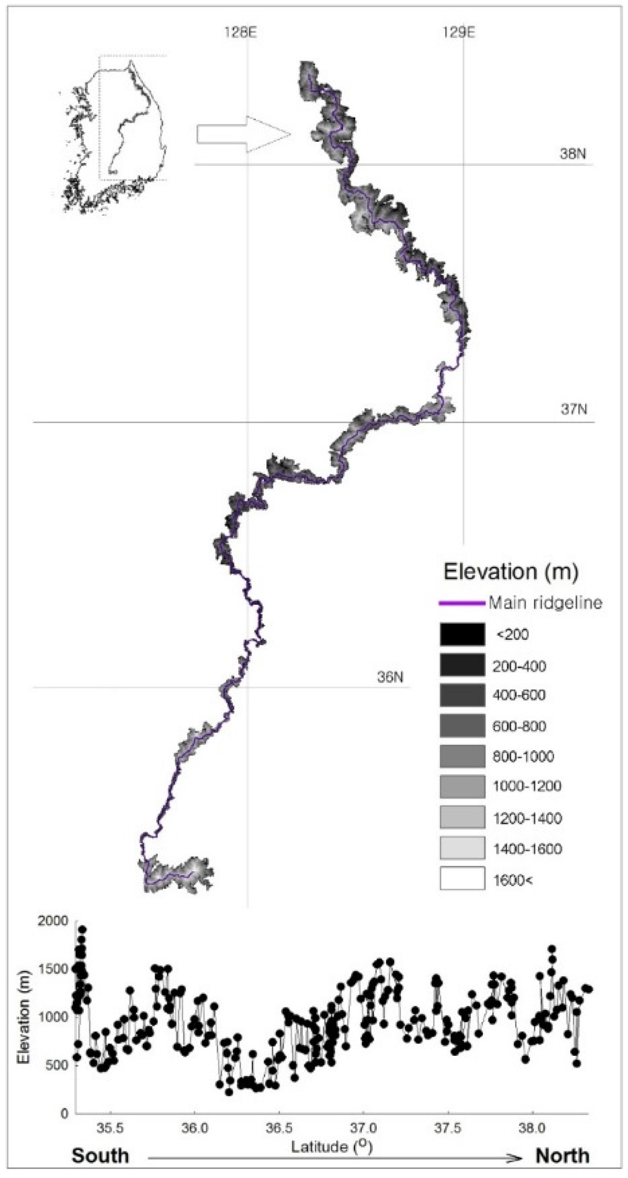
2.1. Study area

We surveyed plant species along the main ridge of the Baekdudaegan Mountains in South Korea (Figure 1). The Baekdudaegan, extending 684 km from Mt Hyangnobong to Mt Jiri, stretch from 35°15′ N, 127°28′ E and 38°22′ N, 129°3′ E with elevation ranging from 200 to 1909 m a.s.l. The protected area of the Baekdudaegan was designated in September 2005 by the Korea Forest Service; the total protected area, including the main ridge, covers 2634 km2 (1712 km2 core districts and 992 km2 buffer districts). The ridge of the Baekdudaegan belongs to core districts and is protected by the Baekdudaegan Protection Act announced by the Korea Forest Service with restrictions on overall activities in the core districts [22]. This also forms a protected area registered with the International Union for Conservation of Nature (IUCN) and is widely recognized as a well-conserved area with an effective protection system [23]. Monthly mean temperature ranges from a minimum of −5.9 °C in January to a maximum of 19.6 °C in August while mean annual precipitation varies from about 1200–2200 mm based on national digital climate maps produced by the National Center of AgroMeteorology, Korea Meteorological Administration [24]. The Baekdudaegan in South Korea belongs to a mountain ecoregion and a temperate deciduous forest biome while the bedrock is composed of granite, granite gneiss and metamorphic sedimentary rocks [22]. The Baekdudaegan is a core site of forest biodiversity in South Korea, containing a total of 1477 plant species belonging to 126 families and 541 genera, which account for 35.2% of the vascular plants in South Korea [23]. The vegetation is categorized into 49 communities, including 42 natural (e.g., Quercus mongolica Fisch. ex Ledeb. community) and seven planted (e.g., Larix kaempferi (Lamb.) Carrière community) vegetation communities. It is divided into four vegetation zones by elevation, namely (1) the temperate deciduous broad-leaved and pine forest dominated by Pinus densiflora Siebold & Zucc. and Rhus trichocarpa Miq. under 550 m, (2) the temperate deciduous broad-leaved and coniferous mixed forest dominated by Abies holophylla Maxim., P. koraiensis Siebold & Zucc., Q. mongolica Fisch. ex Ledeb. and Q. serrata Murray between 550 and 1100 m, (3) sub-alpine coniferous forest dominated by Taxus cuspidata Siebold & Zucc., A. koreana E. H. Wilson and A. nephrolepis (Trautv. ex Maxim.) Maxim. between 1100 and 1600 m, and (4) dwarf sub-alpine forest dominated by Betula ermanii Cham. and P. pumila (Pall.) Regel above 1600 m [22].
Figure 1. Location and topography of the study areas on the ridge of the Baekdudaegan Mountains in South Korea.
Forests 07 00019 g001

2.2. Plant Data and Diversity Indices

A 100 m-wide transect was established in a north–south direction along the ridge of the Baekdudaegan. The ridge was divided into 16 elevations using 100-m intervals extending from 200 to more than 1700 m a.s.l. Field sampling was performed to cover the most common and specific physiognomic vegetation types in each elevational band. However, the sampling efforts were different among elevational bands and were biased to elevational bands with large areas due to the long latitudinal range of the study area (almost 3°) and different areas among elevational bands. Plant data were obtained from a total of 1100 plots within 400 m2 along the 100 m-wide transect from May 2005 to August 2009. The plant species and a cover-abundance scale were recorded within each plot according to the method of Braun-Blanquet [25]. Table S1 lists the plant species and life form checklists at each elevation.
To examine the relationships between plant diversity and elevation or explanatory variables, we calculated four diversity indices using plant data from the field surveys: (1) the total number of species per elevational band (NSB) as a measurement of gamma diversity, (2) the mean number of species per plot in each elevational band (MNSP) as a measurement of alpha diversity, (3) the total estimated number of species per elevational band (ENSB) as estimated gamma diversity and (4) the beta diversity (BETAD) of each elevational band. The NSB was defined as the total number of species that were recorded in each elevational band. We calculated the MNSP as the mean number of species in all plots of each elevational band. The ENSB was defined as the mean value of seven non-parametric species diversity estimators (ACE, ICE, Chao1, Chao2, Jackknife1, Jackknife2 and bootstrap) [26]. The BETAD was also defined as the mean value of eight compositional similarity indices (Classic Jaccard and Sørensen similarity indices, Chao’s Jaccard Raw Abundance-based similarity index and its estimator, Chao’s Sørensen Raw Abundance-based similarity and its estimator, Morisita-Horn similarity index and Bray-Curtis similarity index). Nonparametric species richness estimators for ENSB and similarity indices for BETAD were computed using EstimateS software version 8.2 [27]. All of the diversity indices were computed for three plant groups: total, woody and herbaceous plants. Additionally, the rarefaction approach was used to rectify the bias that was caused by different sample sizes among elevational bands [26,27]. All of the diversity indices were rarefied at the lowest number of samples (n = 26) that were observed in the 1700-m elevational band. Rarefied diversity indices allowed a comparison of the diversity indices of each plant group with an equal number of samples for each elevational band.

2.3. Explanatory Variables

To test the species-area relationships, we calculated the regional area (RA) of each elevational band for the entire mountain range to estimate the habitat area that is available to support the regional species pool. In addition, the three topographic variables of slope, surface area ratio (SAR) and topographic position index (TPI) were calculated to estimate the effects of each elevational band on the plant diversity in the 100-m-wide transects using a triangular irregular network (TIN) model. This model represents a surface as a set of non-overlapping contiguous triangular facets of irregular sizes and shapes [28]. These shapes were based on a digital elevation model (DEM) that was developed from a 1:25,000 digital terrain map. SAR was developed as a method for calculating a type of roughness called rugosity, which is essentially the ratio of study region’s surface area to the planar surface area [29]. TPI was calculated as the slope position relative to the surrounding landscape, with negative values indicating areas that are lower than the surrounding landscape (ravines) and positive values indicating areas that are higher than the surrounding landscape (ridges) [30]. We also calculated the standard deviations (SD) of slope, TPI and SAR in each elevational band as measures of topographic heterogeneity. To perform calculations for the regional area, six topographic characteristics were measured using a DEM with a resolution of 30 m with the 3D Analyst extension in ArcGIS.
This study used two climatic variables, mean annual temperature (MAT) and precipitation (MAP). We used digital climate maps that had been produced by the Korea Meteorological Administration and National Center of Agrometeorology to extract the meteorological parameters for each elevational band [23]. MAT data were dated from 1971 to 2008, and MAP data were dated from 1981 to 2009. The spatial resolution of the raster data was 30 m for MAT and 270 m for MAP. MAT and MAP were calculated for each elevational band in the 100-m-wide transects.
To assess the relationships between the diversity components and productivity, we used the mean annual enhanced vegetation index (EVI) as a surrogate of net primary productivity [31]. MODIS-derived 16-day composite EVI images were downloaded at 500-m resolution between January 2004 and December 2009 and mosaicked together using the MODIS re-projection tool.
In contrast to topographic heterogeneity as a proxy of habitat heterogeneity at a regional level, we also calculated the vegetation structure diversity and vegetation type diversity (VTD) as proxies of habitat heterogeneity at a plot level. To assess the effect of vegetation structure on plant diversity, we calculated the mean percentage covers of the tree (>5 m), subtree (2–5 m), shrub (1–2 m) and herb (<1 m) layers in sampled plots of each elevational band. We also recorded the major vegetation type covering most of each sampled plot based on the dominant tree species (Table S2) and calculated the VTD in each elevational band based on the Shannon-Wiener index as follows:
H = i   = 1 S p i ln p i
where S and pi are the number of vegetation types and the proportion of the ith vegetation type in an elevational band, respectively.
The RA and mean percentage cover data were subjected to log and arc-sine square root transformations for statistical analysis, respectively. Moreover, to reduce the total number of variables and to ensure the orthogonality of variables, four separate principal component analyses (PCAs) were performed on each set of the topographic, SD of topographic, climatic, and vegetation structure variables except for RA, EVI and VTD (Table S3). From each PCA, the first axis was extracted, resulting in the new PCA-derived variables, which were then used in the subsequent data analyses as independent variables. The new PCA-derived variables were named PC1topo, PC1hetero, PC1climate and PC1vegest for topographic variable, topographic heterogeneity, climate and vegetation structure diversity, respectively.

2.4. Data Analysis

Linear and quadratic regression models were fitted to assess the relationships between elevation and four diversity indices of three plant groups. To test the effects of individual variables, such as logRA, PC1topo, PC1hetero, PC1climate, EVI, PC1vegest and VTD, on the elevational patterns of diversity indices, we performed a simple linear regression analysis for each plant group. We also used forward stepwise multiple regression models to establish the relative importance of the explanatory variables for the diversity indices of each plant group. In this study, forward stepwise multiple regressions were used to find a set of independent variables that together provide the best fit for the observed patterns of diversity by minimizing the sum of the squared residuals. All of the linear terms of the explanatory variables were used in the forward stepwise multiple regression analyses. We used PAST version 2.17c for PCA and SPSS version 18.0 for simple linear and forward stepwise multiple regressions.

3. Results

3.1. General Description

A total of 802 plant species belonging to 97 families and 342 genera were recorded along the elevational gradient on the Baekdudaegan (Table 1 and Table S1). More than half of these species were herbaceous (69%; 62 families, 249 genera and 554 species), while woody species accounted for 31% (47 families, 99 genera and 248 species).
Table 1. Observed species richness among total, woody and herbaceous plants for different elevational bands along the ridge of the Baekdudaegan Mountains, South Korea.
Elevational Band (m)Number of PlotsTotalWoodyHerbaceous
2003618886102
3006419393100
40064240106134
5004619588107
60061218101117
70093284126158
800117372138234
900113364127237
1000103389133256
110072355118237
120070366114252
130068337111226
140075320109211
15005423986153
16003819173118
1700261103971
All bands pooled1100802248554
Figure 2. Relationships between elevation and (a) regional area; (b) slope; (c) surface area ratio; (d) topographic position index; (e) standard deviation (SD) of slope; (f) SD of surface area ratio; (g) SD of topographic position index; (h) mean annual temperature; (i) mean annual precipitation; (j) enhanced vegetation index; (k) tree layer cover; (l) subtree layer cover; (m) shrub layer cover; (n) herbaceous layer cover and (o) vegetation type diversity.
Forests 07 00019 g002
Among explanatory variables, with increasing elevation, the RA of the elevational bands increased steeply and then decreased after reaching 800–900 m (Figure 2a). The slope and SAR increased steeply to 700–800 m and then reached a plateau from 800 to 1700 m (Figure 2b,c). TPI generally increased (Figure 2d) and the standard deviations of slope, SAR and TPI had hump-shaped patterns along the elevational gradient (Figure 2e–g). Among climatic variables, MAT decreased monotonically with increasing elevation (Figure 2h), whereas MAP increased (Figure 2i). The EVI as well as tree layer and subtree layer covers generally decreased with elevation (Figure 2j–l). The shrub layer cover decreased from 200–1600 m and then increased steeply to more than 1600 m (Figure 2m). The herbaceous layer cover had two peaks at 200–300 m and 1400–1500 m (Figure 2n). The vegetation type diversity peaked from 700 to 1500 m and had the lowest value from 900 to 1000 m (Figure 2o).

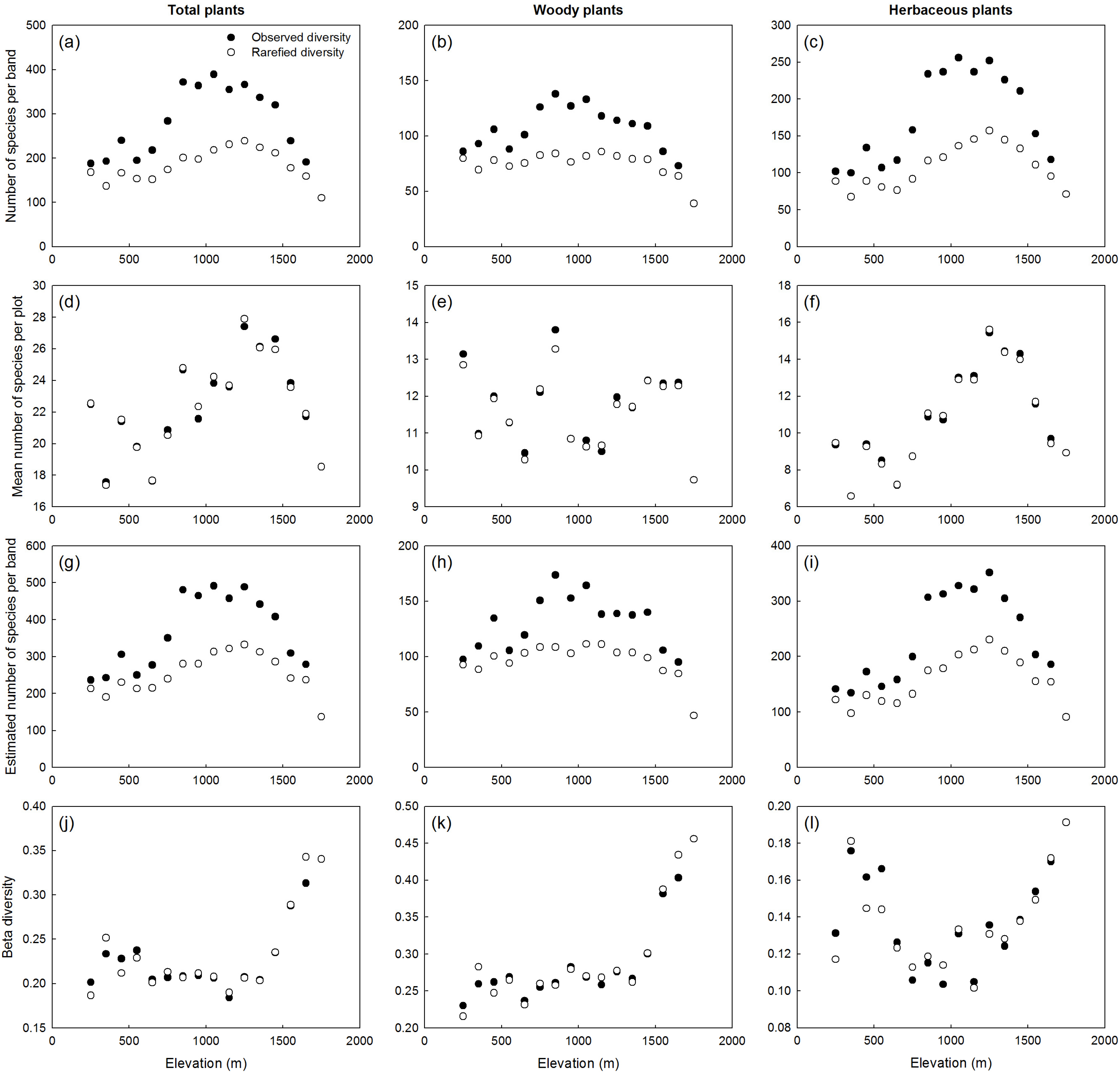
3.2. Elevational Plant Diversity Patterns

The observed NSBs of the total, woody and herbaceous plants showed hump-shaped patterns with maximum richness between 800 m and 1100 m (Table 2, Figure 3a–c). The observed MNSPs for total and woody plants had no significant relationship with elevation; in particular, the MNSP for woody plants showed approximately multimodal patterns with peaks at the 200-, 800- and 1400-m elevational bands (Table 2, Figure 3d,e). However, the observed MNSP for herbaceous plants had both significant linear and quadratic relationships with elevation, and the power of the quadratic model was higher than that of the linear model (Table 2, Figure 3f). The ENSBs for all of the plant groups showed a hump-shaped pattern with maximum richness between 800 and 1300 m (Table 2, Figure 3g–i). The BETADs for two plant groups, except for the herbaceous plants, generally increased with elevation and both the linear and quadratic models were significant (Table 2, Figure 3j–l). Although the explanatory powers of both of the models were somewhat different, similar relationships occurred between observed and rarefied diversity indices with elevation.
Table 2. Relationship between elevation and plant diversity with linear and quadratic models along the ridge of the Baekdudaegan Mountains, South Korea. Rarefied diversity was calculated with the same sample size (n = 26) in each elevational band.
Observed DiversityRarefied Diversity
LinearQuadraticLinearQuadratic
Total
NSB<0.010.77 ***0.040.57 **
MNSP0.160.330.150.34
ENSB0.020.76 ***0.040.64 **
BETAD0.34 *0.78 ***0.38 *0.74 ***
Woody
NSB0.080.84 ***0.20.67 ***
MNSP0.020.020.010.01
ENSB0.050.79 ***0.140.79 ***
BETAD0.61 ***0.85 ***0.61 ***0.83 ***
Herbaceous
NSB0.060.74 ***0.170.59 **
MNSP0.28 *0.50 **0.27 *0.50 *
ENSB0.070.72 ***0.150.62 **
BETAD0.030.61 **0.090.59 **
Significance levels are * p < 0.05; ** p < 0.01; *** p < 0.001. Abbreviations: NSB, number of species per elevational band; MNSP, mean number of species per plot; ENSB, estimated number of species per elevational band; BETAD, beta diversity per elevational band.
Figure 3. Relationships between elevation and plant diversity indices of total, woody and herbaceous plants along the ridge of the Baekdudaegan Mountains, South Korea. Four plant richness indices were used: (ac) the number of species per elevational band; (df) the mean number of species per plot; (gi) the estimated number of species per elevational band, and (jl) the beta diversity per elevational band. Rarefied diversity was calculated with the same sample size (n = 26) in each elevational band.
Forests 07 00019 g003

3.3. Plant Diversity Patterns with Explanatory Variables

The simple linear models yielded similar results between the observed and rarefied diversity patterns (Table 3). The overall diversity indices for all of the plant groups commonly had significant relationships with PC1hetero based on the simple linear models. However, several exceptions occurred (observed and rarefied MNSPs and BETADs for woody plants; rarefied BETAD for total plants). The observed and rarefied MNSPs for woody plants had significant relationships with only VTD in simple linear models. Based on forward stepwise multiple regression models that were used to select the best model, PC1hetero was also the most important explanatory variable in most of the diversity indices for all of the plant groups (Table 4). LogRA or PC1climate was also an important variable for BETADs. For the total plants, the observed BETAD showed a strong relationship with logRA, whereas PC1hetero and PC1climate explained the variation in rarefied BETAD. In addition, VDT was the most important variable for the MNSPs for woody plants even in forward stepwise multiple regression models.
Table 3. Coefficients of determination (R2) and significance levels from simple linear regression models for explanatory variables and diversity indices of total, woody and herbaceous plants along the ridge of the Baekdudaegan Mountains, South Korea. Rarefied diversity was calculated with the same sample size (n = 26) in each elevational band.
logRAPC1topoPC1heteroPC1climateEVIPC1vegestVTD
Observed diversity
Total
NSB0.30 *0.030.61 ***0.030.030.02<0.01
MNSP<0.010.020.26 *0.040.10<0.01<0.01
ENSB0.250.030.62 ***0.020.010.01<0.01
BETAD0.63 ***0.140.30 *0.59 ***0.26 *0.26 *<0.01
Woody
NSB0.66 ***0.010.53 ***0.27 *0.190.120.08
MNSP<0.010.16<0.010.030.040.200.31 *
ENSB0.59 ***<0.010.54 ***0.200.170.100.10
BETAD0.65 ***0.31 *0.160.81 ***0.36 *0.42 **0.03
Herbaceous
NSB0.170.070.58 ***<0.01<0.01<0.010.01
MNSP0.010.110.30 *0.100.100.020.05
ENSB0.130.060.58 ***<0.01<0.01<0.010.01
BETAD0.39 **<0.010.47 **0.140.080.020.02
Rarefied diversity
Total
NSB0.100.010.56 ***<0.01<0.010.01<0.01
MNSP<0.010.020.26 *0.030.11<0.01<0.01
ENSB0.130.020.63 ***<0.01<0.010.01<0.01
BETAD0.60 ***0.140.230.62 ***0.240.33 *<0.01
Woody
NSB0.52 **0.140.43 **0.40 **0.100.28 *0.09
MNSP<0.010.160.010.020.040.180.32 *
ENSB0.62 ***0.060.58 ***0.33 *0.140.170.10
BETAD0.64 ***0.28 *0.120.81 ***0.36 *0.44 **0.01
Herbaceous
NSB0.010.080.47 **0.030.040.010.04
MNSP0.010.110.29 *0.090.100.020.05
ENSB0.030.070.53 ***0.020.04<0.010.02
BETAD0.43 **0.020.43 **0.230.050.040.02
Abbreviations: logRA, log-transformed regional area; PC1topo, PC1 from topographic variables; PC1hetero, PC1 from standard deviations of topographic variables; PC1climate, PC1 from climatic variables; EVI, enhanced vegetation index; PC1vegest, PC1 from vegetation covers; VTD, vegetation type diversity. Table 2 describes abbreviations for diversity indices. Significance levels are * p < 0,05; ** p < 0.01; *** p < 0.001.
Table 4. Results of forward stepwise multiple regression models for the explanatory variables and diversity indices of total, woody and herbaceous plants along the ridge of the Baekdudaegan Mountains, South Korea. Table 2 and Table 3 describe the abbreviations for explanatory variables and diversity indices. Rarefied diversity was calculated with the same sample size (n = 26) in each elevational band.
Plant GroupDependent VariableRegression EquationFR2P
Observed diversity
TotalNSBy = 272.563 + 68.748 PC1hetero22.040.61<0.001
MNSPy = 22.352 + 1.572 PC1hetero4.810.260.046
ENSBy = 351.195 + 89.798 PC1hetero23.260.62<0.001
BETADy = 0.465 − 0.026 logRA24.010.63<0.001
WoodyNSBy = 3.793 + 10.891 logRA + 10.264 PC1hetero21.880.77<0.001
MNSPy = 5.603 + 3.229 VTD6.200.310.026
ENSBy = 16.424 + 11.982 logRA + 14.314 PC1hetero17.330.73<0.001
BETADy = 0.292 − 0.022 PC1hetero + 0.0002 PC1climate89.290.93<0.001
HerbaceousNSBy = 169.563 + 50.018 PC1hetero19.150.580.001
MNSPy = 20.886 − 1.114 logRA + 2.345 PC1hetero7.150.520.008
ENSBy = 226.663 + 66.164 PC1hetero19.690.580.001
BETADy = 0.140 − 0.019 PC1hetero12.190.470.004
Rarefied diversity
TotalNSBy = 182.574 + 28.012 PC1hetero17.920.560.001
MNSPy = 22.399 + 1.610 PC1hetero4.990.260.042
ENSBy = 252.669 + 43.834 PC1hetero24.270.63<0.001
BETADy = 0.233 − 0.022 PC1hetero + 0.0001 PC1climate27.560.81<0.001
WoodyNSBy = 20.258 + 5.982 logRA15.420.520.002
MNSPy = 5.899 + 3.025 VTD6.530.320.023
ENSBy = 41.510 + 6.047 logRA + 7.518 PC1hetero22.470.78<0.001
BETADy = 0.294 − 0.022 PC1hetero + 0.0002 PC1climate61.670.91<0.001
HerbaceousNSBy = 107.844 + 20.365 PC1hetero12.310.470.003
MNSPy = 20.438 − 1.068 logRA + 2.289 PC1hetero6.490.500.011
ENSBy = 157.311 + 32.458 PC1hetero15.890.530.001
BETADy = 0.137 − 0.016 PC1hetero + 0.00004 PC1climate10.920.630.002

4. Discussion

This study explored the patterns of four plant diversity indices and the environmental determinants on an extensive temperate elevational gradient in South Korea. Many previous studies have been restricted to the use of only species richness as a surrogate of biodiversity at each elevational band in their analyses without using other valuable diversity indices, such as the mean number of species and beta diversity. This is because these studies used interpolated species richness as modified from distributional records with secondary data sources, such as the literature [32]. Therefore, our study benefited from exploring the elevational patterns and the drivers with additional valuable diversity indices as related to an empirical data source; these data were collected at a regional scale and were analyzed by comparing the results with many previous studies using secondary data from the literature. Moreover, few studies have analyzed the importance of habitat characteristics in relation to patterns of elevational diversity at a regional scale. Below, we discuss plant diversity patterns with elevation as well as the type of variables, such as regional area, topographic variables, topographic heterogeneity, climate, productivity, vegetation structure diversity and vegetation type diversity. We also explain how these variables may influence the patterns of elevational plant diversity along the ridge of the Baekdudaegan.

4.1. Elevational Plant Diversity Patterns

Our study revealed the different elevational patterns in plant diversity not only among diversity indices and but also among plant groups along the ridge of the Baekdudaegan. We detected hump-shaped patterns of NSBs and ENSBs for all of the plant groups and MNSP only for herbaceous plants, despite different elevational peaks among diversity indices and plant groups. The hump-shaped distribution in elevational patterns of species richness at regional scales is the most commonly observed pattern in many taxa of various ecosystems [7]. At the most general level, our study adds to the growing body of evidence demonstrating that the observed and estimated total number of species per elevational band exhibits strong hump-shaped patterns in mountain ecosystems with changes in elevation. However, the absolute elevations of the diversity peaks vary somewhat among studies [2,4,11,12,13,41]. Moreover, in our study area, previous studies have reported that the most widespread middle-elevation oak forests (e.g., Q. dentata Thunb. forest, Q. mongolica Fisch. ex Ledeb. forest, Q. serrata Murray forest) have the highest woody plant richness [33] and higher herbaceous plant richness than other forest types (e.g., P. densiflora Siebold & Zucc. forest, Robinia pseudoacacia L. forest, Styrax obassia Siebold & Zucc. forest), whereas pine forests (e.g., P. densiflora Siebold & Zucc. forest, P. koraiensis Siebold & Zucc. forest), which are mainly dominant at low and high elevations, have the lowest total species richness [34]. These hump-shaped patterns may reflect these differences of species richness by vegetation types with elevational gradient.
However, the MNSPs of the total and woody plants showed some fluctuation; in particular, the MNSP of woody plants had no clear peak and exhibited a multimodal pattern with the elevational gradient. Such multimodal patterns are rarely observed in nature, considering the large number of elevational gradients that have been studied. Rahbek [7] estimated that approximately 50%, 25%, and 25% of the recorded elevational patterns were hump-shaped, monotonic decreasing and other patterns, respectively. Our results are consistent with those of two recent studies on vascular plants on Mt. Tianshan in central Xinjiang, China [35] and Mt. Seorak in South Korea [36]. First, Sang [35] reported that the total and herbaceous plant species diversity of total, tree, shrub and herbaceous plants showed multimodal patterns along an elevational gradient. He found two or several peaks of plant diversity in the transition zones between vegetation types, and that these patterns were controlled by climatic and soil factors, such as temperature, precipitation, soil water and nutrition, on Mt. Tianshan in China. Lee et al. [36] also revealed different patterns, including monotonic decline as well as hump-shaped and multimodal patterns for the different diversity indices of total, woody and herbaceous plants with elevation on Mt. Seorak in South Korea.
Previous studies frequently reported that, based on the similarity in composition of local assemblages, BETAD increases with increasing latitude [37,38]. Elevation transects have commonly been championed as useful models of larger-scale ecological patterns because they compress marked changes in climate into relatively small distances [21], and the elevational gradient is claimed to parallel the latitudinal gradient [39]. Therefore, the same BETAD patterns between latitudinal and elevational gradients are expected. In the present study, while BETADs in total and woody plants increased with elevation, this was not the case with herbaceous plants. Stevens [40] extended Janzen’s hypotheses to explain the elevational patterns of species richness, under the assumption that climate is more temporally variable at high than at low elevations; one can, therefore, deduce that based on similarity, BETAD increases with increasing elevation [40]. Moreover, the present results for the BETAD patterns of total and woody plants on the Baekdudaegan are consistent with those on the Qilian Mountains of China [41]. However, herbaceous plants did not show an increasing pattern rather than a reversed hump-shaped pattern. This result implies that an extension of Janzen’s hypothesis to an elevational gradient [40] is not applicable for BETAD of herbaceous plants, at least on the ridge of the Baekdudaegan.
Another possibility may be that these differences are caused by differences in dispersal abilities between woody and herbaceous plants. In general, because forest herbs are often poorly dispersed compared with woody species, herbaceous species in particular may tend to be patchily distributed even in a homogeneous environment [42,43]. Restrictions on dispersal of herbaceous species may produce autocorrelated distributions of individuals of each species. Accordingly, elevational bands with larger areas and larger topographic heterogeneities will contain increasingly different sets of herbaceous species. Therefore, one expects that the BETAD of herbaceous species will show a reversed hump-shaped pattern. However, the BETAD of woody species may be mainly governed by an environmental filtering effect such as climate. It is likely that harsh environments at higher elevation make clustering of woody species with similar ecological traits or lineage more readily able to tolerate stressful high-elevation habitats [44].

4.2. Determinants of Elevational Diversity Patterns

In this study, although the explanatory variables that were identified as significant in simple regression analyses were not necessarily identified as contributors to patterns of diversity in multiple regression analyses, the regional area, topographic heterogeneity, climate and vegetation type diversity were included to explain most of the elevational patterns for diversity indices of the plant groups.
First, area has long been recognized as a crucial determinant of patterns of diversity for species growing along an elevational gradient and is believed to have both indirect and direct effects on species diversity [11,45]. Most studies employing transects attempt to control the influence of area by sampling plots of equal area. However, in addition to the direct influence of the area of the sampled plot, local communities can be perceived as dynamic samples drawn from a regional species pool, and the size of the surrounding region can be considered a surrogate for the size of the regional species pool. Romdal and Grytnes [45] used the term “indirect area effect” to describe the effect of regional area on the local pattern of diversity. In this study, we used the regional area as a predictor to explain plant diversity patterns. Our results also indicate that the indirect area effect was important in explaining the elevational patterns for several diversity indices on the ridge of the Baekdudaegan despite some differences in the results between simple and multiple regression analyses. Moreover, several studies found that the observed elevational diversity patterns were largely explained by the amount of available area within elevational bands [45].
Habitat heterogeneity is also considered to be an important variable in shaping patterns of diversity, notably by driving local differences in species distributions and thereby increasing diversity via differences in environmental preferences [46]. An increase in the number of habitat types or greater structural complexity in vegetation can provide more resources than a more uniform environment and may therefore support a greater number of species [47]. Heterogeneity is also thought to have a significant influence on the dynamics and structure of ecological communities [48]. However, although traditionally interpreted as local-scale heterogeneity, habitat heterogeneity also can shape diversity at larger spatial scales. Habitat heterogeneity appears to be less frequently evaluated than other factors in elevational gradient analyses. This may occur because of the difficulties that are associated with measuring this variable and the non-independence with other potential factors such as climate, pedogenic stage, productivity and resource availability [49]. In this study, we used three variables as surrogates of habitat heterogeneity: topographic heterogeneity at a regional scale and vegetation structure diversity and vegetation type diversity at a plot scale. Of these variables, topographic heterogeneity was one of the most important variables for all of the plant groups and diversity indices except for the MNSP of woody plants. However, the MNSP of woody plants was also explained by vegetation type diversity as another proxy of habitat heterogeneity at a plot level. Topography is an important factor regulating biodiversity at the local and regional scales [50], although it was not a significant variable in this study. In particular, topographic heterogeneity can create a complex mosaic of substrates with varying structures, hydrologies and chemistries [51]. Moreover, these factors that were formed by topographic heterogeneity may also affect vegetation patterns by imposing environmental constraints on plant growth and offer a wide variety of different habitats, as well as buffering against climate change [50]. Hofer et al. [52] suggested that topographic heterogeneity is an effective and significant variable that can be used as a proxy of habitat heterogeneity to estimate plant diversity in large agricultural landscapes of Switzerland. In addition, different vegetation types can possess significant differences in plant diversity, and habitats with diverse vegetation types can stochastically harbor more diverse species than those with less diverse vegetation types in habitats with the same areas [53]. In this study, even though the VTD was only related to the MNSP of woody plants, this result indicates the possibility that, based on dominant tree species, VTD can be used as a surrogate of habitat heterogeneity to predict the MNSP of woody plants on the ridge of the Baekdudaegan. Although we did not use light heterogeneity including solar radiation, or soil heterogeneity in moisture, nutrients and soil type, which are resources that directly influence plant diversity in this study, undoubtedly the availability of these resources influence plant establishment, community succession and patterns of diversity [49]. Indeed, in the present study area, Černý et al. [33] have reported that soil nutrients and solar radiation are important variables that can be used to explain plant diversity and that the relative importance of individual predictors was most probably determined by environmental stress, which changes along the elevational gradient. Moreover, at large scales such as the scale of our study area, vegetation type and structure generally have evolved in a particular climate with specific precipitation and temperature characteristics. This occurs because climate can indirectly influence changes in vegetation type and structure by controlling soil factors relevant to nutrient availability and pedogenic stage and also modify the disturbance regime [14], although we could not find direct relationships between climate and vegetation type or structure in this study. Therefore, vegetation diversity indices such as VDT and vegetation structure diversity in this study may indirectly reflect the effects of other potential factors such as soil nutrients, solar radiation and climate.
In general, climate is an obvious factor that may control species distribution and diversity in many areas [14]. This study suggested that significant relationships exist between climate and beta diversity; however, as observed with the other discussed variables, these effects are not necessarily the same between the results from simple and multiple regression analyses. In addition, climate had a significant effect on the observed beta diversity of woody plants between both the simple and multiple regressions in this study. Lenoir et al. [54] reported that when comparing forests with similar internal environmental variation and using the same sampling unit size, one might expect that macroclimate differences affecting gamma diversity will be the primary cause of the corresponding differences in the beta diversity of woody plants. Moreover, if the explanation of the limited carrying capacity holds, climatic differences could also modulate beta diversity by changing the tree density of forests. Some studies have also suggested that the combined effects of climate and other variables, such as habitat heterogeneity and soil characteristics, may provide an explanation for beta diversity [35,55]. In this study, the climate also showed a combined effect with topographic heterogeneity rather than an individual effect in multiple regression models.
Among environmental drivers, primary productivity is frequently cited as a fundamental determinant of diversity pattern, although controversy remains as to the nature of the relationship and the potential underlying mechanisms [56]. Studies using remote sensing-based vegetation indices as surrogates of primary productivity have found significant productivity-diversity relationships, suggesting that such estimates can be used to evaluate patterns of diversity [14]. However, our study found little support for primary productivity in shaping the patterns of plant diversity on the ridge of the Baekdudaegan. This suggests that the relationships between productivity and elevation and between productivity and diversity may be more complex than previously thought. Among elevational gradient studies, the location of peak productivity is often qualitatively asserted to be based on inverse or largely incongruent trends in precipitation and temperature [57]. These results demonstrate that such assertions may be misleading.

5. Conclusions

The plant diversity patterns along an elevational gradient on the ridge of the Baekdudaegan were different among both diversity indices and plant groups confirming our first expectation. These had: hump-shaped, reversed hump-shaped, increasing, multimodal, and no relationships. Of these elevational patterns, the hump-shaped pattern was the predominant type for the observed and estimated number of species as a measurement of gamma diversity. The mean number of species per plot, as a measurement of alpha diversity in an elevational band, showed no relationships or multimodal patterns for total and woody plants whereas herbaceous plants showed hump-shaped pattern. Beta diversity depicted increasing patterns for total and woody plants and a reversed hump-shaped pattern for herbaceous plants. Explanatory variables that were identified as significant under simple regression analyses were not necessarily identified as contributors to patterns of diversity using multiple regression analyses. However, regional area, habitat heterogeneity, such as topographic heterogeneity and vegetation type diversity, and climate were included to explain most of the elevational diversity patterns of all of the plant groups. In particular, habitat heterogeneity was the most important variable for explaining the elevational patterns of plant diversity along the ridge of the Baekdudaegan. Elevational patterns of diversity differed among plant groups and also among different diversity indices. In addition, elevational patterns of plant diversity may be primarily explained by habitat heterogeneity on the ridge of the Baekdudaegan. This occurs because more heterogeneous and diverse habitats can support more coexisting species despite different responses of plant groups to the environment such as potential dispersal ability and resource availability.

Supplementary Materials

Supplementary materials can be found at https://www.mdpi.com/1999-4907/7/1/19.

Acknowledgments

We thank Keun-Wook Lee and Sang-Hyouk Seo for invaluable help during the fieldwork and data analysis in this study. Thanks are also due to Hyun-Je Cho and Sang-Gon Park for their support and encouragement. This paper forms part of the “Korea Big Tree Project” funded by the Korea Green Promotion Agency, Korea Forest Service.

Author Contributions

Chang-Bae Lee and Jung-Hwa Chun generated the main ideas and analyzed the data. Chang-Bae Lee led the writing. Authors read and approved the final manuscript.

Conflicts of Interest

The authors declare no conflict of interest.

References

  1. Gaston, K.J. Global patterns in biodiversity. Nature 2000, 405, 220–227. [Google Scholar] [CrossRef] [PubMed]
  2. Grytnes, J.A.; Vetaas, O.R. Species richness and altitude: A comparison between null models and interpolated plant species richness along the Himalayan altitudinal gradient, Nepal. Am. Nat. 2002, 159, 294–304. [Google Scholar] [CrossRef] [PubMed]
  3. Zhang, X.Y.; Ma, K.M.; Anand, M.; Fu, B.J. Do generalized scaling laws exist for species abundance distribution in mountains? Oikos 2006, 115, 81–88. [Google Scholar] [CrossRef]
  4. Acharya, B.K.; Chettri, B.; Vijayan, L. Distribution pattern of trees along an elevational gradient of Eastern Himalaya, India. Acta Oecologica 2011, 37, 329–336. [Google Scholar] [CrossRef]
  5. Swenson, N.G.; Erickson, D.L.; Mi, X.; Bourg, N.A.; Forero-Montaña, J.; Ge, X.; Howe, R.; Lake, J.K.; Liu, X.; Ma, K.; et al. Phylogenetic and functional diversity alpha and beta diversity in temperate and tropical tree communities. Ecology 2012, 93, S112–S125. [Google Scholar] [CrossRef] [Green Version]
  6. Legendre, P.; Borcard, B.; Peres-Neto, P.R. Analyzing beta diversity: Partitioning the spatial variation of community composition data. Ecol. Monogr. 2005, 75, 435–450. [Google Scholar] [CrossRef]
  7. Rahbek, C. The role of spatial scale and the perception of large-scale species-richness patterns. Ecol. Lett. 2005, 8, 224–239. [Google Scholar] [CrossRef]
  8. Field, R.; Hawkins, B.A.; Cornell, H.V.; Currie, D.J.; Diniz-Filho, J.A.F.; Guégan, J.F.; Kaufman, D.M.; Kerr, J.T.; Mittelbach, G.G.; Oberdorff, T.; et al. Spatial species-richness gradients across scales: A meta-analysis. J. Biogeogr. 2009, 36, 132–147. [Google Scholar] [CrossRef]
  9. Gentili, R.; Armiraglio, S.; Sgorbati, S.; Baroni, C. Geomorphological disturbance affects ecological driving forces and plant turnover along an altitudinal stress gradient on alpine slopes. Plant Ecol. 2013, 214, 571–586. [Google Scholar] [CrossRef]
  10. Legendre, P.; Dale, M.R.T.; Fortin, M.J.; Casgrain, P.; Gurevitch, J. Effects of spatial structures on the results of field experiments. Ecology 2004, 85, 3202–3214. [Google Scholar] [CrossRef]
  11. Rahbek, C. The elevational gradient of species richness: A uniform pattern? Ecography 1995, 18, 200–205. [Google Scholar] [CrossRef]
  12. Grau, O.; Grytnes, J.A.; Birks, H.J.B. A comparison of altitudinal species richness patterns of bryophytes with other plant groups in Nepal, Central Himalaya. J. Biogeogr. 2007, 34, 1907–1915. [Google Scholar] [CrossRef]
  13. Wang, Z.; Tang, Z.; Fang, J. Altitudinal patterns of seed plant richness in the Gaoligong Mountains, south-east Tibet, China. Divers. Distrib. 2007, 13, 845–854. [Google Scholar] [CrossRef]
  14. Rowe, R.J. Environmental and geometric drivers of small mammal diversity along elevational gradients in Utah. Ecography 2009, 32, 411–422. [Google Scholar] [CrossRef]
  15. Wu, Y.; Colwell, R.K.; Rahbek, C.; Zhang, C.; Quan, Q.; Wang, C.; Lei, F. Explaining the species richness of birds along a subtropical elevational gradient in the Hengduan Mountains. J. Biogeogr. 2013, 40, 2310–2323. [Google Scholar] [CrossRef]
  16. Sanders, N.J. Elevational gradients in ant species richness: Area, geometry, and Rapoport’s rule. Ecography 2002, 25, 25–32. [Google Scholar] [CrossRef]
  17. Jetz, W.; Rahbek, C. Geographic range size and determinants of avian species richness. Science 2002, 297, 1548–1551. [Google Scholar] [CrossRef] [PubMed]
  18. Whittaker, R.H. Vegetation of the Siskiyou Mountains, Oregon and California. Ecol. Monogr. 1960, 30, 280–338. [Google Scholar] [CrossRef]
  19. Sfenthourakis, S.; Panitsa, M. From plots to islands: Species diversity at different scales. J. Biogeogr. 2012, 39, 750–759. [Google Scholar] [CrossRef]
  20. Lomolino, M.V. Elevational gradients of species-density: Historical and prospective views. Glob. Ecol. Biogeogr. 2001, 10, 3–13. [Google Scholar] [CrossRef]
  21. Körner, C. The use of ‘altitude’ in ecological research. Trends Ecol. Evol. 2007, 22, 569–574. [Google Scholar] [CrossRef] [PubMed]
  22. Kong, W.S. Biogeography of Korea Plants, 2nd ed.; GeoBook Publishing: Seoul, Korea, 2007. (In Korean) [Google Scholar]
  23. Korea Forest Research Institute. Ecological Aspects of Baekdu Mountains in Korea and Delineation of Their Management and Conservation area; Korea Forest Research Institute: Seoul, Korea, 2003. (In Korean) [Google Scholar]
  24. Yun, J.I. Agroclimatic maps augmented by a GIS technology. Korean J. Agric. For. Meteorol. 2010, 12, 63–73. [Google Scholar] [CrossRef]
  25. Braun-Blanquet, J. Plant Sociology; Hafner Publishing Company: New York, NY, USA, 1965. [Google Scholar]
  26. Colwell, R.K.; Mao, C.X.; Chang, J. Interpolating, extrapolating and comparing incidence-based species accumulation curves. Ecology 2004, 85, 2717–2727. [Google Scholar] [CrossRef]
  27. Colwell, R.K. Estimate S: Statistical Estimation of Species Richness and Shared Species from Samples. Available online: http://purl.oclc.org/estimates (accessed on 20 September 2015).
  28. Speckmann, B.; Snoeyink, J. Easy triangle strips for TIN terrain models. Int. J. Geograph. Inf. Sci. 2001, 15, 379–386. [Google Scholar]
  29. Jenness, J.S. Calculating landscape surface area from digital elevation models. Wildl. Soc. Bull. 2004, 32, 829–839. [Google Scholar] [CrossRef]
  30. Jenness, J.S. Topogrphic Position Index (tpi_jen.avx) Extension for ArcView 3.x. Available online: http://www.jennessent.com/arcview/tpi.htm (accessed on 10 September 2015).
  31. Adhikari, D.; Barik, S.K.; Upadhaya, K. Habitat distribution modeling for reintroduction of Ilex khasiana Purk., a critically endangered tree species of northeastern India. Ecol. Eng. 2012, 40, 37–43. [Google Scholar] [CrossRef]
  32. Oommen, M.A.; Shanker, K. Elevational species richness patterns emerge from multiple local mechanisms in Himalayan woody plants. Ecology 2005, 86, 3039–3047. [Google Scholar] [CrossRef]
  33. Černý, T.; Doležal, J.; Janeček, Š.; Šrůtek, M.; Valachovič, M.; Petřík, P.; Altman, J.; Bartoš, M.; Song, J.S. Environmental correlates of plant diversity in Korean temperature forests. Acta Oecologica 2013, 47, 37–45. [Google Scholar] [CrossRef]
  34. Lee, C.B.; Cho, H.J.; Chun, J.H.; Song, H.K.; Kim, H.H. Variations in species and functional plant diversity among forest types on the ridge of the Baekdudaegan Mountains, South Korea. J. Agric. Life Sci. 2013, 47, 147–162. [Google Scholar]
  35. Sang, W. Plant diversity patterns and their relationships with soil and climatic factors along an altitudinal gradient in the middle Tianshan Mountain area, Xinjiang, China. Ecol. Res. 2009, 24, 303–314. [Google Scholar] [CrossRef]
  36. Lee, C.B.; Chun, J.H.; Ahn, H.H. Elevational patterns of plant richness and their drivers on an Asian mountain. Nord. J. Bot. 2014, 32, 347–357. [Google Scholar] [CrossRef]
  37. Koleff, P.; Lennon, J.J.; Gaston, K.J. Are there latitudinal gradients in species turnover? Glob. Ecol. Biogeogr. 2003, 12, 483–498. [Google Scholar] [CrossRef]
  38. Qian, H.; Ricklefs, R.E. A latitudinal gradient in large-scale beta diversity for vascular plants in North America. Ecol. Lett. 2007, 10, 737–744. [Google Scholar] [CrossRef] [PubMed]
  39. Begon, M.; Harper, J.L.; Townsend, C.R. Ecology: Individuals, Populations and Communities; Blackwell Science: Oxford, UK, 1990. [Google Scholar]
  40. Stevens, G.C. The elevational gradient in altitudinal range: An extension of Rapoport’s latitudinal rule to altitude. Am. Nat. 1992, 140, 893–911. [Google Scholar] [CrossRef] [PubMed]
  41. Wang, G.; Zhou, G.; Yang, L.; Li, Z. Distribution, species diversity and life-form spectra of plant communities along an altitudinal gradient in the northern slope of Qilianshan Mountans, Gansu, China. Plant Ecol. 2002, 165, 169–181. [Google Scholar] [CrossRef]
  42. Peterken, G.F.; Game, M. Historical factors affecting the number and distribution of vascular plant species in the woodlands of central Lincolnshire. J. Ecol. 1984, 72, 155–182. [Google Scholar] [CrossRef]
  43. Singleton, R.; Gardescu, S.; Marks, P.L.; Geber, M.A. Forest herb colonization of postagricultural forests in central New York State, USA. J. Ecol. 2001, 89, 325–338. [Google Scholar] [CrossRef]
  44. Webb, C.O. Exploring the phylogenetic structure of ecological communities: An example for rain forest trees. Am. Nat. 2000, 156, 145–155. [Google Scholar] [CrossRef] [PubMed]
  45. Romdal, T.S.; Grytnes, J.A. An indirect area effect on elevational species richness patterns. Ecography 2007, 30, 440–448. [Google Scholar] [CrossRef]
  46. Moeslund, J.E.; Arge, L.; Bøcher, P.K.; Nygaard, B.; Svenning, J.C. Geographically comprehensive assessment of salt-meadow vegetation-elevation relations using LiDAR. Wetlands 2011, 31, 471–482. [Google Scholar] [CrossRef]
  47. Chase, J.M.; Leibold, M.A. Ecological Niches: Linking Classical and Contemporary Approaches; University of Chicago Press: Chicago, IL, USA, 2003. [Google Scholar]
  48. Vivian-Smith, G. Microtopographic heterogeneity and floristic diversity in experimental wetland communities. J. Ecol. 1997, 85, 71–82. [Google Scholar] [CrossRef]
  49. Laliberté, E.; Grace, J.B.; Huston, M.A.; Lambers, H.; Teste, F.P.; Turner, B.L.; Wardle, D.A. How does pedogenesis drive plant diversity? Trends Ecol. Evol. 2013, 28, 331–340. [Google Scholar] [CrossRef] [PubMed]
  50. Moeslund, J.E.; Arge, L.; Bøcher, P.K.; Dalgaard, T.; Svenning, J.C. Topography as a driver of local terrestrial vascular plant diversity patterns. Nord. J. Bot. 2013, 31, 129–144. [Google Scholar] [CrossRef]
  51. Bledsoe, B.P.; Shear, T.H. Vegetation along hydrologic and edaphic gradients in a North Carolina coastal plain creek bottom and implications for restoration. Wetlands 2000, 20, 126–147. [Google Scholar] [CrossRef]
  52. Hofer, G.; Bunce, R.G.H.; Edwards, P.J.; Szerencsits, E.; Wagner, H.H.; Herzog, F. Use of topographica variability for assessing plant diversity in agricultural landscapes. Agric. Ecosyst. Environ. 2011, 142, 144–148. [Google Scholar] [CrossRef]
  53. Chiarucci, A.; de Dominicis, V.; Wilson, J.B. Structure and floristic diversity in permanent monitoring plots in forest ecosystems of Tuscany. For. Ecol. Manag. 2001, 141, 201–210. [Google Scholar] [CrossRef]
  54. Lenoir, J.; Gégout, J.C.; Guisan, A.; Vittoz, P.; Wohlgemuth, T.; Zimmermann, N.E.; Dullinger, S.; Pauli, H.; Willner, W.; Grytnes, J.A.; et al. Cross-scale analysis of the region effect on vascular plant species diversity in southern and northern European mountain ranges. PLoS ONE 2010, 5, e15743. [Google Scholar] [CrossRef] [PubMed]
  55. Novillo, A.; Ojeda, R.A. Elevational patterns in rodent diversity in the dry Andes: Disentangling the role of environmental factors. J. Mammal. 2014, 95, 99–107. [Google Scholar] [CrossRef]
  56. Hawkins, B.A.; Field, R.; Cornell, H.V.; Currie, D.J.; Guégan, J.F.; Kaufman, D.M.; Kerr, J.T.; Mittelbach, G.G.; Oberdorff, T.; O’Brien, E.; et al. Energy, water, and broad-scale geographic patterns of species richness. Ecology 2003, 84, 3105–3117. [Google Scholar] [CrossRef]
  57. McCain, C.M. The mid-domain effect applied to elevational gradients: Species richness of small mammals in Costa Rica. J. Biogeogr. 2004, 31, 19–31. [Google Scholar] [CrossRef]

