Data Assimilation in Forest Inventory: First Empirical Results

Abstract

Data assimilation techniques were used to estimate forest stand data in 2011 by sequentially combining remote sensing based estimates of forest variables with predictions from growth models. Estimates of stand data, based on canopy height models obtained from image matching of digital aerial images at six different time-points between 2003 and 2011, served as input to the data assimilation. The assimilation routines were built on the extended Kalman filter. The study was conducted in hemi-boreal forest at the Remningstorp test site in southern Sweden (lat. 13°37′ N; long. 58°28′ E). The assimilation results were compared with two other methods used in practice for estimation of forest variables: the first was to use only the most recent estimate obtained from remotely sensed data (2011) and the second was to forecast the first estimate (2003) to the endpoint (2011). All three approaches were validated using nine 40 m radius validation plots, which were carefully measured in the field. The results showed that the data assimilation approach provided better results than the two alternative methods. Data assimilation of remote sensing time series has been used previously for calibrating forest ecosystem models, but, to our knowledge, this is the first study with real data where data assimilation has been used for estimating forest inventory data. The study constitutes a starting point for the development of a framework useful for sequentially utilizing all types of remote sensing data in order to provide precise and up-to-date estimates of forest stand parameters.

1. Introduction

Accurate information about forest stands is one of the keys to successful forest management and for efficient wood supply to the forest industry. Modern planning tools, such as the Heureka system [1], can be applied to support decision making in forestry. These tools rely on accurate information about the stands in the target forest area and have the potential to provide solutions to the spatiotemporal planning problem that go beyond what can be achieved by human intuition [2].

Traditionally in many countries, stand-level forest information has been collected through recurrent campaigns. That is, every 10–20 years data have been collected in the field from all stands in a forest holding in order to update the information. However, the transfer to digital databases in combination with the increasing flow of low-cost data that are becoming regularly provided through remote sensing motivates a shift towards continuous updating. Several new remote sensing techniques are emerging, and we are entering an unprecedented era of information richness. Modern 3D remote sensing techniques like point clouds from laser scanning [3] and stereo-view image matching of digital aerial images (denoted “image matching”) [4] are being rapidly developed and applied. Digital aerial images are regularly acquired in many countries, and it has recently been shown that point clouds from aerial images can be used to estimate canopy heights and correlated variables with good accuracy [5,6,7,8]. In a similar way, accurate forest height estimates can be obtained frequently from interferometric SAR data [9,10] as well as from radargrammetry [11]. This remote sensing development might imply a paradigm shift regarding how information is collected and compiled for purposes of forest management planning.

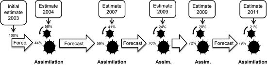
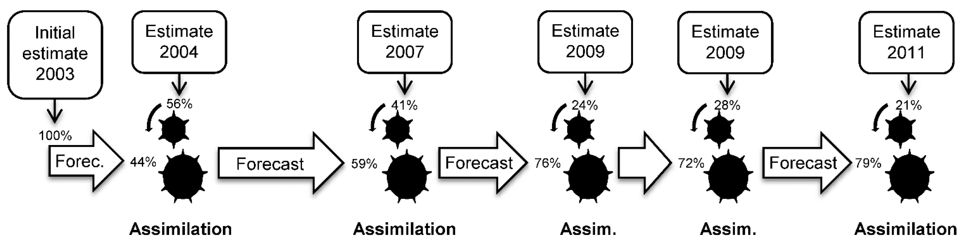
Data assimilation can be used to continuously combine models and new sensor data in an optimal way, offering great potential for making use of new sources of forest information. Existing information about a forest area is forecasted using a model that provides an estimate for the date of the next data acquisition and an estimate of the precision of the forecasted information. Thus, the precision of the forecasted information can be compared with the precision of the new information. In the assimilation step, the two sources of information are combined through weights that are inversely proportional to their uncertainties (Figure 1). The combined estimate is then forecasted to the time-point of the next data acquisition, and repeated when new data become available.

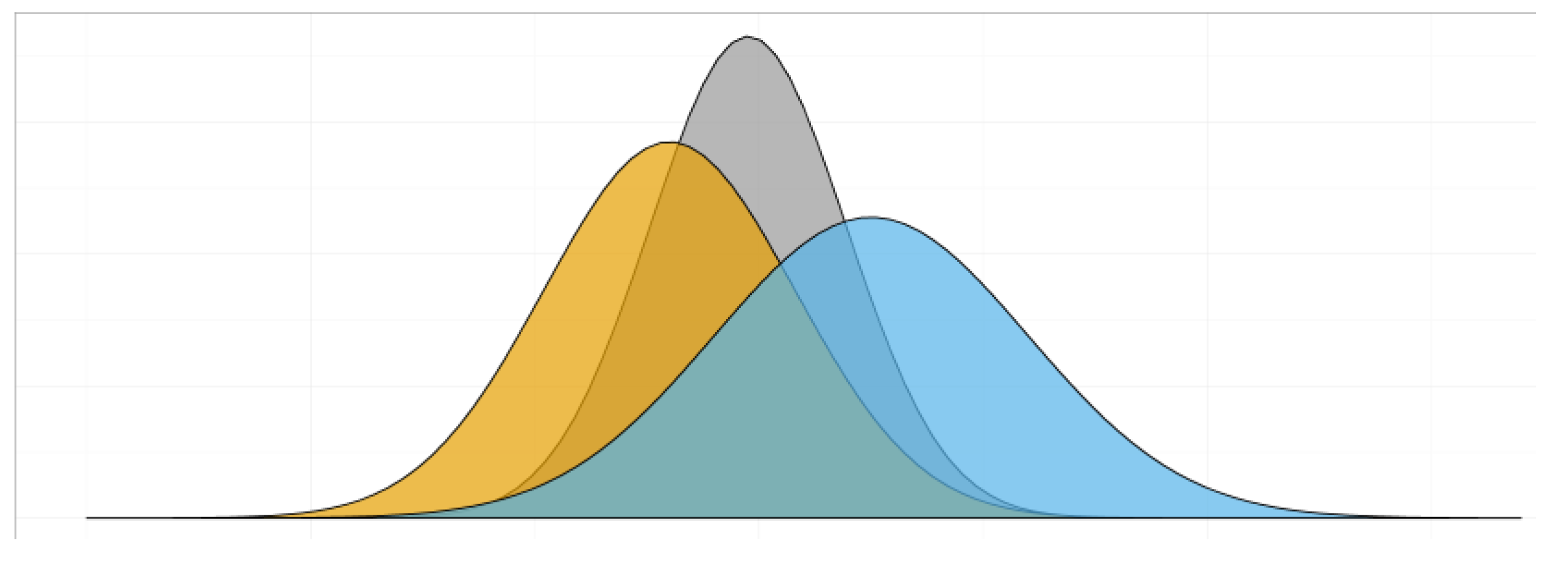
Figure 1. An illustration of the basic principle of data assimilation applied to a Gaussian model and estimate. The figure shows how the prior forecast (the center of the orange distribution) is updated to the posterior forecast (the center of the grey distribution) when a new estimate (the center of the blue distribution) is taken into account. Notice that the grey distribution is narrower than the orange distribution, indicating that the posterior forecast is more precise (i.e., the estimate has lower variance) than the prior forecast.

Figure 1. An illustration of the basic principle of data assimilation applied to a Gaussian model and estimate. The figure shows how the prior forecast (the center of the orange distribution) is updated to the posterior forecast (the center of the grey distribution) when a new estimate (the center of the blue distribution) is taken into account. Notice that the grey distribution is narrower than the orange distribution, indicating that the posterior forecast is more precise (i.e., the estimate has lower variance) than the prior forecast.

The success of data assimilation in areas such as meteorology is well documented [12]. Data assimilation of time series of satellite data has also been used in research studies for calibration of physical models of ecosystem functions [13]. Such models typically produce estimates of ecosystem variables such as gross primary production, net primary production and ecosystem respiration [14]. Data assimilation techniques have also been proposed for operational forest inventory [15,16,17,18], but we are not aware of any previous data assimilation studies where estimates like those usually produced and employed for forest management planning have been made using real data.

However, in order to realize the potential in the context of forest inventory and management, the data assimilation techniques need to be adapted to this field of application. This involves development of new growth models from which not only growth predictions can be made but also the uncertainty of those models can be ascertained. All new estimates from remote sensing or field surveys should be used to adjust the forecasted forest information to the extent motivated by the uncertainties of the new estimates as compared to the uncertainties of the forecasts. Thus, through data assimilation, forest planning would benefit from having up-to-date and accurate information available as input to its different planning processes, from long-term strategic planning to short-term optimization of the value chains linking forests with forest industry.

Two common approaches to data assimilation are Kalman filtering [19] and Bayesian methods [20]. Kalman filters assume that the errors of the forecasts and the new measurements based on sensor data are normally distributed whereas Bayesian methods can handle any distribution of errors. In the basic setting, the Kalman filter assumes linear forecasting models, so that the variance of forecasted variables can be calculated without approximation. However, several further developments of the Kalman filter are available as well, such as the extended Kalman filter which uses a Taylor approximation to linearize non-linear prediction models. Bayesian methods assume the true state to be a random variable and predict entire joint probability distributions of the variables of interest.

In a previous simulation study made by our research group [15], several challenges for applying data assimilation to forest information were identified. These included non-linear growth models, temporal correlation of errors from growth models, poorly known uncertainty of estimates, spatiotemporally correlated inventory errors, and the need in some cases to handle discrete data, such as individual trees within description units. Thus, any future system for data assimilation in forestry would need to be developed through a series of research studies where the different challenges are addressed.

The objective of the present study was to present our first empirical results of the application of data assimilation to forest stand data. In our previous study [15], the results were based on theoretical assumptions and the article provided case examples of the potential benefits of applying data assimilation. In the present study, we applied the data assimilation technique to empirical estimates based on point clouds from image matching from six time-points obtained over an eight year period (2003–2011) calibrated with forest estimates from circular field plots. Estimates were compiled for three variables: stem volume (V), basal area (BA) and Lorey’s mean height (H_L). Data assimilation using the extended Kalman filter was compared to two methods used in practice for estimation of forest variables: (i) estimates of the target variables using point clouds from image matching from the most recent time-point (denoted “most recent estimate”) and (ii) forecasting the stand development with growth models from the initial state estimate (denoted “forecast”).

2. Materials and Methods

2.1. Study Area

The study was carried out at the forest estate Remningstorp in southwestern Sweden (lat. 13°37′ N; long. 58°28′ E). This 1500 ha estate is covered primarily by well-managed, productive forest. The forest is dominated by Norway spruce (Picea abies) and Scots pine (Pinus sylvestris), with some deciduous forest of mainly birch (Betula pendula and Betula pubescens). Generally, the area is rather flat, with ground elevations ranging from 120 to 145 m above sea level.

2.2. Field Data

In this study, field data were applied for three different purposes: (i) for developing models linking the remotely sensed data with the ground conditions for the target variables (V, BA, H_L), (ii) for developing growth models, and (iii) for validating the results at the endpoint of the data assimilation period.

For the development of models estimating the state of the target variables from the remote sensing data, we used field data from sample plots (denoted “training plots”) distributed across the Remningstorp study area. Training plots were available from two different field campaigns during the study period (data set 1 and 2 in Figure 2). All trees greater than 4 cm diameter at breast height on the plots were calipered, and a sub-sample of the trees was selected for measurements of height and age. Site index (SI) [21] was also assessed on the plots, using the Swedish system for site index based on ground- and field-layer vegetation as indicators of site productivity. Lorey’s mean height (H_L) [22], basal area (BA) and stem volume (V) [23] were calculated for the plots using all trees greater than 4 cm in diameter at breast height. The stem volume was defined as the total volume of the entire stem above the stump, including bark but excluding branches. In Table 1, a summary of the training plot data available for the development of remote sensing based models is given.

Table 1. Field inventories of training plots used for the development of predictive models estimating the state of the target variables from the remote sensing data.

No	Inv. Year	No of Plots	Radius (m)	V (m3/ha) min/mean/max	BA (m2/ha) min/mean/max	HL (m) min/mean/max
1	2004	849	10	0/277/1050	0/28/80	0/19/34
2	2010	247	10	0/202/697	0/22/60	0/16/33

V = Stem volume, BA = Basal area, H_L = Lorey’s mean height, based on all calipered trees greater than 4 cm diameter at breast height.

Table 1. Field inventories of training plots used for the development of predictive models estimating the state of the target variables from the remote sensing data.

No	Inv. Year	No of Plots	Radius (m)	V (m3/ha) min/mean/max	BA (m2/ha) min/mean/max	HL (m) min/mean/max
1	2004	849	10	0/277/1050	0/28/80	0/19/34
2	2010	247	10	0/202/697	0/22/60	0/16/33

V = Stem volume, BA = Basal area, H_L = Lorey’s mean height, based on all calipered trees greater than 4 cm diameter at breast height.

Figure 2. Overview of the study area, the location of the field inventoried training plots, and the validation plots used for assimilation. Data set 1 consists of 849 field plots located in a regular grid of 40 m within the cross-hatched area. ^©Lantmäteriet I2014/00764.

Figure 2. Overview of the study area, the location of the field inventoried training plots, and the validation plots used for assimilation. Data set 1 consists of 849 field plots located in a regular grid of 40 m within the cross-hatched area. ^©Lantmäteriet I2014/00764.

The field data used for developing the growth models were derived from the Swedish National Forest Inventory (NFI) [24]. The NFI each year lays out approximately 10,000 field plots across the land area of Sweden. A majority of the plots are permanent and are revisited every fifth year. The permanent plots from the NFI were used for developing the growth models and the corresponding models for estimating the variance of the growth predictions (see Appendix A).

The third set of field data was the large plots (denoted “validation plots”) used for validating the results of the data assimilation and the two methods used in practice for estimating forest variables (most recent estimate and forecast). The validation plots were selected from a larger dataset of 52 plots with 40 m radius whose positions had initially been located in the interior of fairly homogeneous stands. After having removed all plots that had been subject to cutting or major damages during the study period, as well having omitted the only multi-storied stand, nine plots remained. The nine validation plots (Table 2, Figure 2) were classified into four different forest type classes for which different growth models based on the Swedish NFI data were used. The forest type class was based on the conditions at the time-point of validation (2011). The composition was recorded as spruce stand if more than 65% of the total stem volume was Norway spruce, pine stand if more than 65% of the total stem volume was Scots pine, mixed conifer stand if more than 65% of the total stem volume was conifer, and mixed stand if the total stem volume of broadleaved trees was between 35 and 65%. None of the validation plots had, according to the field inventories, been subject to management (such as thinning or clear-felling) during the period from the first acquisition of images used to the last. All the validation plots (except two) were inventoried in the same growth season as the last aerial images were acquired. The two other plots inventoried during the growth season of 2012 and 2013 were back-casted to the growth season of the field inventory (2011), using the growth models developed in this study.

Table 2. Summary of the validation plots, i.e., the nine large plots with 40 m radius that were used to validate the results of the data assimilation, at growth season 2011.

ID	Inv. Growth Season 1	SI (m/100 years)	Age (years)	HL (m)	V (m3/ha)	BA (m2/ha)	Forest Type Class
10	2011	25	39	21.5	389	39.3	Spruce stand
116	2011	30	55	25.3	501	43.4	Spruce stand
151	2011	31	44	19.8	283	29.3	Spruce stand
211	2011	32	41	21.6	308	30.5	Spruce stand
212	2011	32	40	20.2	241	26.4	Mixed stand
325	2011	31	43	22.2	386	37.0	Spruce stand
351	2011	31	46	20.5	265	27.1	Spruce stand
515	2012	25	26	12.1	115	20.6	Mixed stand
517	2013	30	30	13.1	185	30.8	Mixed stand

¹ Growth season when the plot was measured in field.

Table 2. Summary of the validation plots, i.e., the nine large plots with 40 m radius that were used to validate the results of the data assimilation, at growth season 2011.

ID	Inv. Growth Season 1	SI (m/100 years)	Age (years)	HL (m)	V (m3/ha)	BA (m2/ha)	Forest Type Class
10	2011	25	39	21.5	389	39.3	Spruce stand
116	2011	30	55	25.3	501	43.4	Spruce stand
151	2011	31	44	19.8	283	29.3	Spruce stand
211	2011	32	41	21.6	308	30.5	Spruce stand
212	2011	32	40	20.2	241	26.4	Mixed stand
325	2011	31	43	22.2	386	37.0	Spruce stand
351	2011	31	46	20.5	265	27.1	Spruce stand
515	2012	25	26	12.1	115	20.6	Mixed stand
517	2013	30	30	13.1	185	30.8	Mixed stand

¹ Growth season when the plot was measured in field.

2.3. Remote Sensing Data

Aerial images were acquired with the Intergraph Z/I Imaging Digital Mapping Camera (DMC) system [25] operated by Lantmäteriet (Swedish National Land Survey) for six different survey campaigns with partial or complete coverage of the study site (Table 3). All datasets were acquired at 4800 m above ground level (a.g.l.) except for the 2003 dataset which was acquired at 3000 m a.g.l., resulting in a ground sampling distance of approximately 0.48 m and 0.30 m, respectively. The images were acquired with 60% along-track overlap and 30% across-track overlap, resulting in at least one stereo model for each position on the ground. The images were block triangulated using bundle adjustment and radiometrically corrected by Lantmäteriet, as part of their operational aerial image production, creating a pan-sharpened false colour composite image with 8-bit radiometric resolution.

Table 3. Digital aerial images and training plots used for modeling the target variables.

Acquisition Date	Growth Season 1	Leaf-on/leaf-off	Altitude (m a.g.l.)	Field Ref. Data Set 2	No. of Training Plots Used
13 October 2003	2003	leaf-on	3000	1	361
28 June 2005	2005	leaf-on	4800	1	416
26 May 2007, 3 June 2007	2006	leaf-on	4800	1	258
1 September 2009	2009	leaf-on	4800	2	214
2 May 2010	2009	leaf-off	4800	2	214
23 May 2012	2011	leaf-on	4800	2	166

¹ Refers to whether the acquisition was performed before or after the 15th of June. See section Estimation of forest state from aerial image matching data for details. ² Refers to Table 1.

Table 3. Digital aerial images and training plots used for modeling the target variables.

Acquisition Date	Growth Season 1	Leaf-on/leaf-off	Altitude (m a.g.l.)	Field Ref. Data Set 2	No. of Training Plots Used
13 October 2003	2003	leaf-on	3000	1	361
28 June 2005	2005	leaf-on	4800	1	416
26 May 2007, 3 June 2007	2006	leaf-on	4800	1	258
1 September 2009	2009	leaf-on	4800	2	214
2 May 2010	2009	leaf-off	4800	2	214
23 May 2012	2011	leaf-on	4800	2	166

¹ Refers to whether the acquisition was performed before or after the 15th of June. See section Estimation of forest state from aerial image matching data for details. ² Refers to Table 1.

Image matching was performed using the SURE software [26,27] to produce point cloud data for each dataset. SURE generates a height value for each point using cost-based matching, similar to the semi-global matching method [28]. All possible stereo pairs were used, so that both along-track and cross-track stereo images were incorporated. The point clouds from all stereo-matched image pairs were merged into one point cloud with a point density ranging from 2 to 46 points/m² (mean 8 points/m²) depending on the amount of overlap, the height of acquisition, and object occlusion within the 10 m radius training plots. Finally, the height values of the point cloud were transformed from height above sea level to height above ground level by subtracting a digital terrain model (DTM). The DTM used to normalize the photogrammetric point cloud was created from airborne laser scanning (ALS) data acquired using a Leica ALS 60/23 on April 21, 2011 under leaf-off conditions. The DTM used was the national DTM from Lantmäteriet; its grid size is 2 m and its vertical accuracy (RMS) is 0.2 m [29] and the density of the ALS point cloud used to create the DTM was 0.7 last returns/m².

In this study, an area based approach [30] was used. Metrics describing the point cloud data, such as height distribution and spatial density characteristics, were calculated for every training plot using Fusion software [31]. For the validation plots, raster of each metric was calculated using a grid cell size of 18 m × 18 m, which corresponds to the size of training plot i.e., 314 m².

2.4. Estimation of Forest State from Aerial Image Matching Data

The state of each validation plot was estimated for each image acquisition using the corresponding raster with metrics. Estimation models were trained with training plots, namely data sets 1 and 2 described in Table 1. In order to obtain as good temporal matches as possible, sample plot data were either fore- or back-casted for short time periods to correspond to the time-points of the image acquisitions. This was done using growth models in the forestry planning and analysis system Heureka [1,32]. In southern Sweden, the growth of tree-shoots occurs mainly in June. Therefore, if the images were acquired after the 15th of June, the growth for that particular year was included when the field reference data were computed. For example, the last images (acquired the 23rd of May 2012) will be defined as belonging to growth season 2011, as they were acquired before the breaking point (15th of June). Therefore, we consistently denote the last estimate to be from year 2011 in this study to avoid confusion. Plots that had been subject to logging operations in the time between the field inventory and the remote sensing acquisition were identified through management operations registers provided by the land manager. Affected plots were excluded from the training data, thus resulting in a different number of training plots used for the different acquisitions. Linear regression was applied for modeling Lorey’s mean height (H_L) and non-linear regression for modeling stem volume (V) and basal area (A), using the aerial imagery metrics as predictors. First, model expressions and metrics were chosen using studies of correlation and regression residuals of the reference data surveyed in 2010 and metrics from the aerial images acquired in 2010 (Equations (1)–(3)).

$$H_L={\mathsf{\beta }}_0+{\mathsf{\beta }}_{1}P95+{\mathsf{\beta }}_{2}D+\mathsf{\epsilon }$$

(1)

$$V=\exp \left({\mathsf{\beta }}_3+{\mathsf{\beta }}_{4}P95+{\mathsf{\beta }}_5\ln \left(P95\right)\right)+\mathsf{\epsilon }$$

(2)

$$BA=\text{exp}\left({\mathsf{\beta }}_6+{\mathsf{\beta }}_{7}P30+{\mathsf{\beta }}_8\ln \left(P95\right)\right)+\mathsf{\epsilon }$$

(3)

where P30 and P95 are the 30th and 95th percentiles of the height distribution of image matching points at each plot and D is the ratio of matched points with heights larger than 2 m above ground to all matched points at each plot. Second, the parameters β were then re-estimated for each remaining time-point of aerial images and corresponding reference data. Third, the state of H_L, V and BA for each of the raster elements in the validation plots was estimated at each time-point using the developed models (Equations (1)–(3)) and, for each time-point, the corresponding data and parameter estimates. The residual variances of V and BA were not constant, rather there were increasing trends with respect to the predicted values. As accurate error variance estimates are crucial in the assimilation model, predictive models of the error standard deviations for V and BA and each time-point were developed using linear regression. In other words, models predicting the residual standard deviation from the predicted value of each respective variable were developed. These models were fitted using data of standard deviations calculated for residuals of ten equal intervals of predicted values.

2.5. Data Assimilation

In this study, we applied the extended Kalman filter [19] for the data assimilation. Only univariate models were used. For simplicity, influential factors such as SI, tree species classification and age were assumed to be measured without error to simplify the modeling. We limited the study in this way in order to more easily interpret causes and effects as well as to compare the usefulness of applying data assimilation for estimation of the three different target variables.

Data assimilation was used for modeling the target variables over time using remote sensing data for adjusting the development given by the growth model. Figure 3 shows a flow chart describing the forecasting and assimilation steps in this study. The notations in this article are the same as in [15].

Figure 3. Illustration of the data assimilation procedure used in this study. The years state the growth season for each remote sensing data acquisition. The percentage is an example of the Kalman Gain, i.e., the amount of information that is included from each source when assimilating. The Kalman Gain value is different for each 18 m × 18 m pixel within the validation plot. There were two acquisitions with growth season 2009 and, therefore, no forecast of the growth was needed between these two.

Figure 3. Illustration of the data assimilation procedure used in this study. The years state the growth season for each remote sensing data acquisition. The percentage is an example of the Kalman Gain, i.e., the amount of information that is included from each source when assimilating. The Kalman Gain value is different for each 18 m × 18 m pixel within the validation plot. There were two acquisitions with growth season 2009 and, therefore, no forecast of the growth was needed between these two.

The development over time of the target variable can thus be formulated as:

$$X_t=f\left(x_{t-1},W_t,t-1\right)=x_{t-1}+g\left(x_{t-1},t-1\right)+W_t$$

(4)

where the random variable $X_t$ denotes the state of the target variable at time $t$. The model describes the conditional distribution of $X_t$, given that the observed value of the variable at time $t-1$ was $x_{t-1}$. Thus, the forecasted value at time $t$ was given by the previous value, to which the expected growth $g\left(x_{t-1},t-1\right)$ and a random term $W_t$) were added. The growth models were developed through regression analysis. Details about the methods used for developing the growth models, and the corresponding model outputs, are given in Appendix A.

The growth was estimated for a five-year period; predictions for any shorter periods were obtained through computing a share corresponding to the share of the length of the prediction period. Model precision was assessed through analyzing the variance of the residual errors. It was found that the residuals were heteroscedastic and thus a separate model was applied for estimating the variance of the predictions. This was made by dividing the dataset into groups based on the predicted values and deriving a simple linear regression model for the variance prediction (see

Table A3. Relationships for estimations of the residual standard deviation (SD) as a function of predicted increment. $SD=\mathsf{\alpha }+\mathsf{\beta }\mathsf{Ŷ}$.

	Spruce Stands		Pine Stands		Mixed Conifer Stands		Mixed Stands
Function	α	β	α	β	α	β	α	β
Volume increment, Vi	13.67	0.147	8.68	0.248	14.58	0.113	11.20	0.260
Basal area increment, BAi	1.92	0.183	1.43	0.263	1.83	0.260	2.65	0.096
Mean height increment, Hi	1.55	−0.113	1.34	−0.131	1.46	−0.103	1.71	−0.133

). We assumed the random term $W_t$ to be normally distributed with zero mean and a variance $q_t^2$ that is dependent on the previous state as well as on time; $q_t=\mathsf{\alpha }+\mathsf{\beta }·g\left(x_{t-1},t-1\right)$, where $t\ge 1$ and $\mathsf{\alpha }$ and $\mathsf{\beta }$ are parameters used for estimating the standard deviation of the residual errors. The parameters were different for the three target variables and for different forest type classes.

The deviations between the state of the target variable and estimates of it—based on remotely sensed data—were assumed to be independent normally distributed random variables. These normal distributions were assumed to have zero mean and time-dependent variances according to:

$$Z_t=x_t+V_t$$

(5)

where $Z_t$ is the (random) estimator, $x_t$ is the true state at time-point $t$, and $V_t$ is a random deviation with zero mean and variance, $r_t^2$, which is estimated from the residual errors obtained in connection with the development of estimators for the target variables based on the remotely sensed data, and ${\tilde{z}}_t$ is used as notation for the actual value observed of $Z_t$. Similarly, ${\tilde{x}}_t$ is used as notation for the actual value obtained through the growth predictions, i.e., ${\tilde{x}}_t=f\left({\widehat{x}}_{t-1},0,t-1\right)$, where ${\widehat{x}}_{t-1}$ is the assimilated variable at time-point $t-1$; its variance is denoted $p_{t-1}^2$. In case no estimates are made at time-point $t$, the assimilated variable ${\widehat{x}}_t$ will obtain the value ${\tilde{x}}_t$ and the variance ${\tilde{p}}_t^2=a_t^2{p}_{t-1}^2+q_t^2$. This is a consequence of the use of first order Taylor linearization, in connection with the extended Kalman filter, to linearize the growth model in order to compute the variance. Thus, $a_t=\frac{d}{dx}f\left({\widehat{x}}_{t-1},0,t-1\right)$, or in other words, $a_t$ is the partial derivative of the growth model with respect to the target variable.

In case an estimate is made at time-point $t$, the forecast and the estimate are weighted inversely proportional to the variances to obtain the assimilated variable, i.e.,

$${\widehat{x}}_t=\left(1-K_t\right){\tilde{x}}_t+K_t{\tilde{z}}_t$$

(6)

with the Kalman gain $K_t=\frac{{\tilde{p}}_t^2}{{\tilde{p}}_t^2+r_t^2}$. If the estimator (Equation (5)) has considerable variance then the Kalman gain becomes almost zero, implying that the estimate does not contribute to the assimilation. On the other hand, if the estimator is very precise, then the Kalman gain becomes almost 1, implying that the forecast does not contribute much to the assimilation. Equation (6) is based on the assumption that ${\tilde{x}}_t$ and ${\tilde{z}}_t$ are independent. Further, the variance of the assimilated variable is:

$$p_t^2=\left(1-K_t\right){\tilde{p}}_t^2.$$

(7)

The assimilation steps were conducted for each raster element (18 m × 18 m). For purposes of comparison, we also estimated the state of the validation plots based on two methods used in practice for estimation of forest variables: use of only the most recent remotely sensed data trained with simultaneously surveyed training plots (Table 1, data set 2), and forecasting of the first estimate using growth models. Both these methods and the assimilation were performed on single raster cells and the mean value of the raster cells with its center within the validation plots was calculated for the year of validation (2011). Figure 4 shows a flowchart of the implementation in the code of the data assimilation framework.

Figure 4. Flowchart of the implementation of the data assimilation framework.

Figure 4. Flowchart of the implementation of the data assimilation framework.

Validation of the three methods (assimilation, most recent estimate, and forecast) was made by calculating the deviation ($e_i$) from the field measured value for the nine validation plots at the last time-point. For each method, the deviations were calculated by subtracting the field measured value from the plot mean value of the intersecting raster cells. In addition, the root mean squared error ($RMSE$) and mean deviation ($MD$) was calculated for the three target variables and methods as:

$$RMSE=\sqrt{\frac{1}{n}{\displaystyle \sum }_{i=1}^n{e}_i^2}$$

(8)

$$MD=\frac{1}{n}{\displaystyle \sum }_{i=1}^n{e}_i$$

(9)

3. Results and Discussion

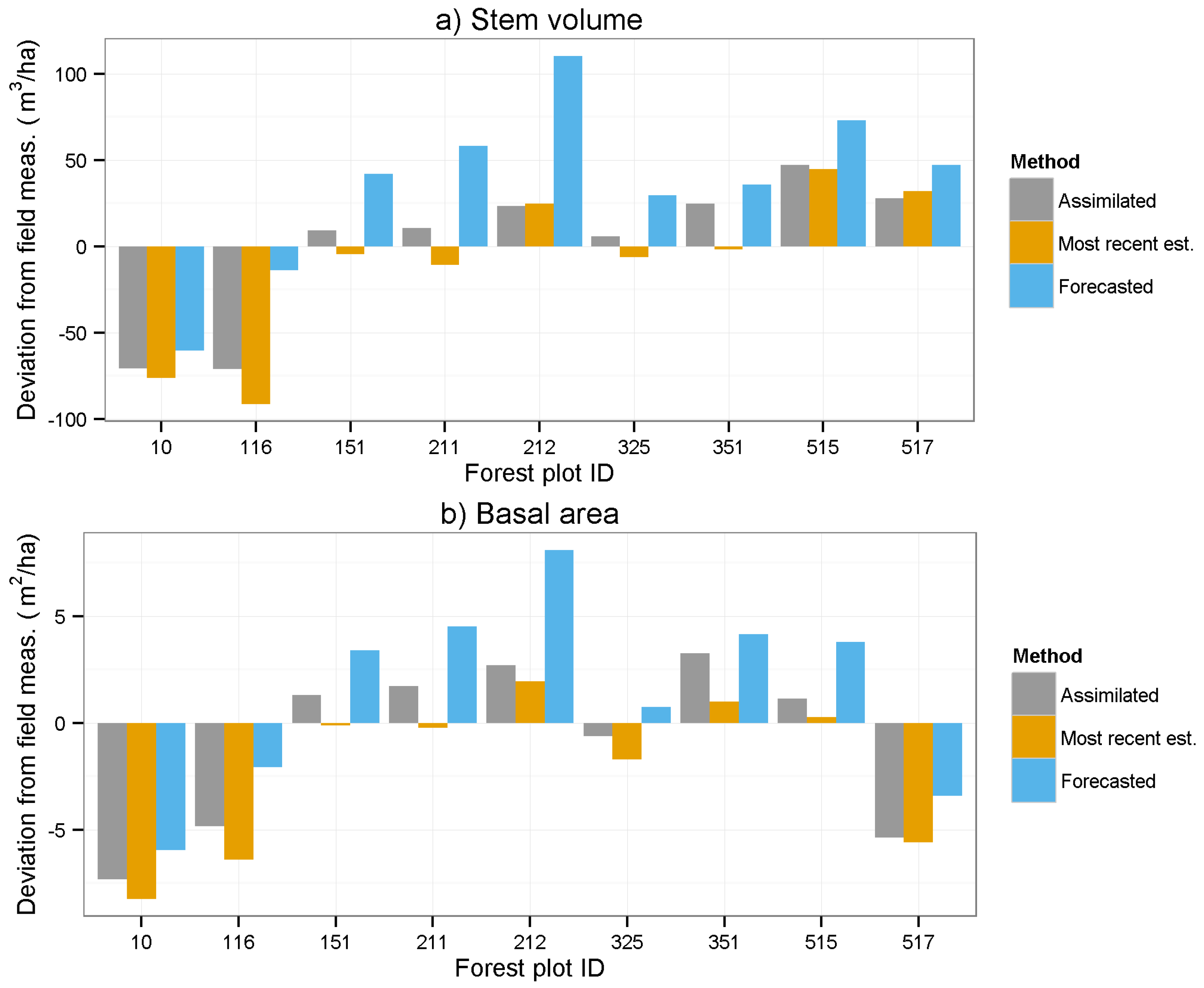
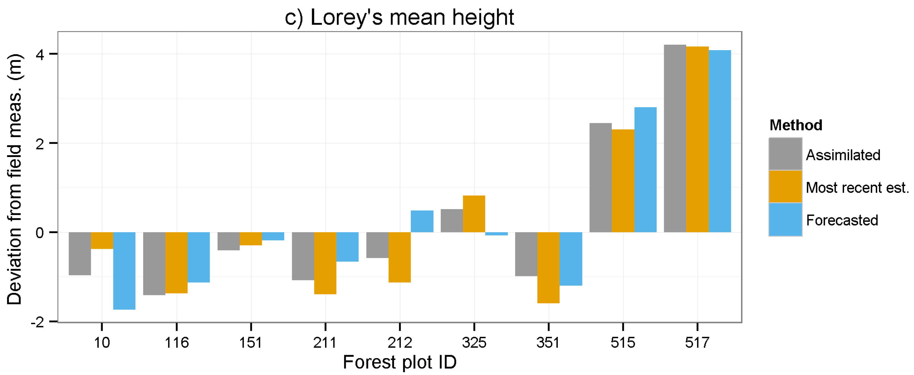
The initial state (2003) was estimated from point clouds obtained from image matching. The validation was made with field data for the 40 m radius validation plots reflecting the state in 2011. Figure 5 shows the deviation from the field measured value for each of the three methods (i.e., assimilation, most recent estimate, forecasting) for the nine validation plots. Table 4 shows the $RMSE$ of the deviation from the field measurements and Table 5 shows the corresponding mean deviation ($MD$). A positive $MD$ means that the plot value is on average overestimated. It can be seen that the $RMSEs$ are smaller using data assimilation compared to forecasting the value from the first (initial state) remote sensing prediction. The full strength of data assimilation will probably first be seen when data from multiple sources are combined. For example, if data are first acquired using airborne laser scanning (ALS) and later acquired with a technique that has lower accuracy, we will be able to update the high accuracy acquisition from the ALS with new data. In a similar way, the data assimilation framework can be used for maintaining information from earlier high quality measurements, for example from field visits, and combining it, rather than replacing it, with new information from remote sensing.

Figure 5. Deviation at year 2011 between field measurement and estimates of (a) stem volume; (b) basal area, and (c) Lorey’s mean height using different methods. A positive value means that the plot has an overestimated value.

Figure 5. Deviation at year 2011 between field measurement and estimates of (a) stem volume; (b) basal area, and (c) Lorey’s mean height using different methods. A positive value means that the plot has an overestimated value.

Table 4. Root mean squared error (RMSE) of the deviation from the field measurement 2011 for the nine assimilated plots. In parentheses is relative RMSE.

Target Variable	Assimilated	Most Recent Estimate	Forecasted
V	40.1 (13.5%)	44.7 (15.0%)	58.5 (19.7%)
BA	3.80 (12.0%)	4.05 (12.8%)	4.49 (14.2%)
HL	1.81 (9.3%)	1.86 (9.6%)	1.86 (9.5%)

Table 4. Root mean squared error (RMSE) of the deviation from the field measurement 2011 for the nine assimilated plots. In parentheses is relative RMSE.

Target Variable	Assimilated	Most Recent Estimate	Forecasted
V	40.1 (13.5%)	44.7 (15.0%)	58.5 (19.7%)
BA	3.80 (12.0%)	4.05 (12.8%)	4.49 (14.2%)
HL	1.81 (9.3%)	1.86 (9.6%)	1.86 (9.5%)

Table 5. Mean deviation ($MD$) from the field measurement 2011 for the nine assimilated plots. A positive $MD$ means that the value is on average overestimated compared to the field measurements. In parentheses is relative $MD$.

Target Variable	Assimilated	Most Recent Estimate	Forecasted
V	0.73 (0.3%)	−10.0 (−3.4%)	35.7 (12.0%)
BA	−0.89 (−2.8%)	−2.12 (−6.7%)	1.47 (4.7%)
HL	0.19 (1.0%)	0.12 (0.6%)	0.27 (1.4%)

Table 5. Mean deviation ($MD$) from the field measurement 2011 for the nine assimilated plots. A positive $MD$ means that the value is on average overestimated compared to the field measurements. In parentheses is relative $MD$.

Target Variable	Assimilated	Most Recent Estimate	Forecasted
V	0.73 (0.3%)	−10.0 (−3.4%)	35.7 (12.0%)
BA	−0.89 (−2.8%)	−2.12 (−6.7%)	1.47 (4.7%)
HL	0.19 (1.0%)	0.12 (0.6%)	0.27 (1.4%)

The results of the validation shows that the accuracy of estimates are similar to other studies of image matching based forest inventory [5,6]. Table 4 and Table 5 show that the assimilated values on average for all stands and variables are better than the most recent estimates, as well as the forecasted estimates. The only exception is that the mean deviation of Lorey’s mean height is lower when using only the most recent estimate. This might be explained by the fact that the photogrammetric point cloud contains particularly accurate information about tree height, and then the gain by data assimilation to reduce noise is less [15]. It is also evident from Figure 5 that two of the mixed stands (515 and 517) had comparatively large over estimates of the canopy height. This might be because broadleaved trees have more leaves and branches in the upper part of the canopy than cone-shaped spruces. Thus, developing separate regression models for different tree species groups might improve the results in future studies.

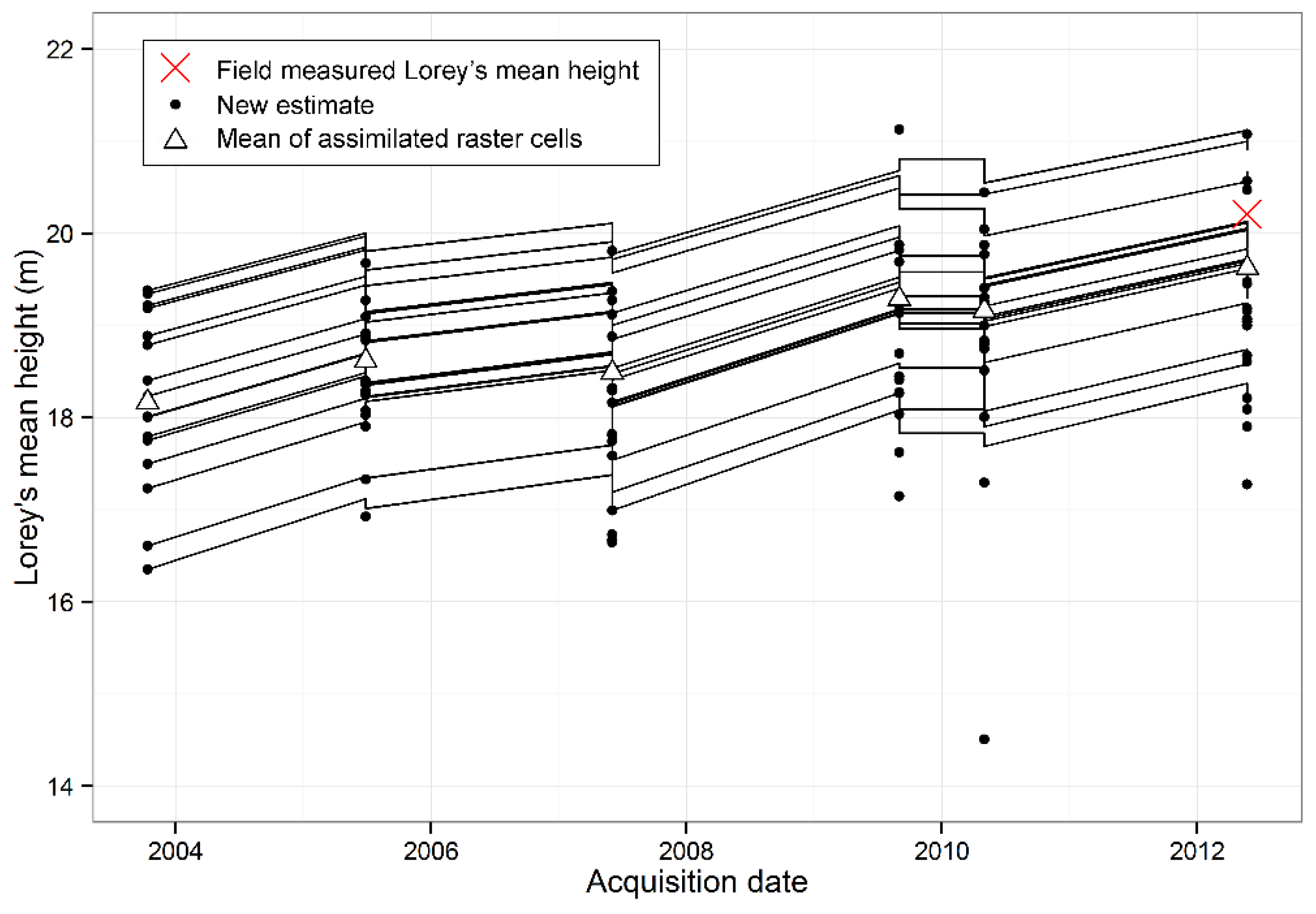
Figure 6 shows the growth of validation plot 212. Each line represents one raster cell within the 40 m radius validation plot. The black dots represent remote sensing based estimates. In the fifth acquisition (2 May 2010), there is one clear outlier at 14.5 m, but the assimilation remained stable despite this. The result of the last assimilation (the rightmost triangle) should be compared with the field measured value (the red cross). It should also be noticed that the acquisition dates are shown on the x-axis, but it is the growth season that determines the growth prediction, and, therefore, the slope is different between the acquisitions.

Figure 6. Data assimilation of Lorey’s mean height on validation plot 212. The black dots are the estimates from remote sensing where each dot represents one 18 m × 18 m raster cell within the validation plot. The triangles are the mean value of the assimilation for each time-point. The red cross is the field measured Lorey’s mean height for the same growth season (2011) as the last acquisition. The black lines are the current estimate for each raster cell. Note that the lines jump either up or down depending on the outcome of the assimilation at each acquisition time-point.

Figure 6. Data assimilation of Lorey’s mean height on validation plot 212. The black dots are the estimates from remote sensing where each dot represents one 18 m × 18 m raster cell within the validation plot. The triangles are the mean value of the assimilation for each time-point. The red cross is the field measured Lorey’s mean height for the same growth season (2011) as the last acquisition. The black lines are the current estimate for each raster cell. Note that the lines jump either up or down depending on the outcome of the assimilation at each acquisition time-point.

In this study, the data are all from the same remote sensing method, i.e., point clouds from image matching of aerial images. Therefore, it is likely that the estimation errors are correlated, which would imply that too much weight is being put on the forecasted information as compared to the new information. This could explain why data assimilation did not perform much better than using information from the most recent estimate (Table 4). Methods to compensate for this will be developed in future studies but requires non-standard filters for the data assimilation. During the course of the study, a test was made where smaller weights were consistently given to the forecasted values in the assimilation step as compared to the weights assigned by the Kalman filter. This led to improved assimilation results, which indicates that the issue of correlated errors needs to be more carefully addressed in future studies.

In a future version of the data assimilation application, the models for prediction of the stand attributes ought to be evaluated in a simultaneous setting to handle cross-correlated errors across models. However, in the present study, we analyzed the different growth characteristics separately over a short time period using simple growth models where the non-static predictors (V, BA, H_L) were not used as predictor variables across the growth models to reduce cross-correlation effects in the forecasts.

The first images were from growth season 2003 and the last from 2011. Thus, the assimilation period is rather short (eight years) considering the time perspective in Nordic forestry where the rotation period is typically 80–100 years. In an operational case, we would have a model that is continuously updated when new data become available and probably spans over much longer time periods than eight years. The starting point for the assimilation is an estimate based on the first aerial images. The short time period might give fairly good growth predictions; however, since the initial state itself is an estimate, it is difficult to evaluate how the forecasts perform.

In this study, the assimilation was conducted on 18 m × 18 m raster cells. Further research is needed to investigate at what level the assimilation should be performed. An alternative could be to assimilate directly at stand level. However, the modeling units for the growth forecasts and the estimates based on remotely sensed data need to correspond, and it must be possible to acquire high quality field reference data for purposes of modeling. These issues point towards raster based approaches to data assimilation being more straightforward than stand based approaches. However, procedures need to be developed where the precision of aggregated raster elements can be estimated.

We are entering an era with a frequent flow of data from different sources and of different types. An example of this is the potential availability of several optical and radar satellite images per year, point clouds from digital photogrammetry with a few years’ time interval, and laser scanning data with five to ten years’ time interval. In addition, there will also be different types of field reference data, for example, from field plots, harvesters and ground based laser scanners. The data assimilation technique offers a potential method for utilizing all of these data sources, even if some of these sources would not be sufficient for use in operational forest planning when used alone. The combination of these different data sources will be the subject of further studies.

4. Conclusions

This study presents the first empirical results of data assimilation applied to the estimation of forest variables. A system for data assimilation has been developed, implemented and validated. The input to the data assimilation was canopy height models obtained from image matching of digital aerial images at six different time points during the growth season between 2003 and 2011. The study showed that data assimilation of stem volume, basal area and Lorey’s mean height resulted in marginally better accuracy than estimates made from the last available aerial images, but substantially better accuracy than estimates from the first available aerial images forecasted to the endpoint. There is a strong potential to further develop the data assimilation concept. Among the benefits are that data from all relevant remote sensors can be utilized in proportion to their information content and complement each other in the assimilation. Furthermore, there is no need for each new remote sensing data set to cover the whole area of interest. When remote sensing data are missing for an area of interest at any time point, predictions for that area will be obtained by the growth models. In a similar way, a database with field reference plots could be continuously updated with new ground truth data, for example, from harvesters, even if the whole area of interest is not covered each time. The field reference plots will be forecasted, and old plots with cutting or suspected damages according to records and/or remote sensing change detection will be omitted when the next set of remotely sensed data becomes available.

References

1. Wikström, P.; Edenius, L.; Elfving, B.; Eriksson, L.O.; Lämås, T.; Sonesson, J.; Öhman, K.; Wallerman, J.; Waller, C.; Klintebäck, F. The Heureka forestry decision support system: An overview. Math. Comput. For. Nat. Resour. Sci. 2011, 3, 87–94. [Google Scholar]
2. Baskent, E.Z.; Keles, S. Spatial forest planning: A review. Ecol. Model. 2005, 188, 145–173. [Google Scholar] [CrossRef]
3. Næsset, E.; Gobakken, T.; Holmgren, J.; Hyyppä, H.; Hyyppä, J.; Maltamo, M.; Nilsson, M.; Olsson, H.; Persson, A.; Söderman, U. Laser scanning of forest resources: The Nordic experience. Scand. J. For. Res. 2004, 19, 482–499. [Google Scholar] [CrossRef]
4. Leberl, F.; Irschara, A.; Pock, T.; Meixner, P.; Gruber, M.; Scholz, S.; Wiechert, A. Point Clouds: Lidar versus 3D Vision. Photogramm. Eng. Remote Sens. 2010, 76, 1123–1134. [Google Scholar] [CrossRef]
5. Bohlin, J.; Wallerman, J.; Fransson, J.E.S. Forest variable estimation using photogrammetric matching of digital aerial images in combination with a high-resolution DEM. Scand. J. For. Res. 2012, 27, 692–699. [Google Scholar] [CrossRef]
6. Gobakken, T.; Bollandsås, O.M.; Næsset, E. Comparing biophysical forest characteristics estimated from photogrammetric matching of aerial images and airborne laser scanning data. Scand. J. For. Res. 2015, 30, 73–86. [Google Scholar] [CrossRef]
7. Pitt, D.G.; Woods, M.; Penner, M. A comparison of point clouds derived from stereo imagery and airborne laser scanning for the area-based estimation of forest inventory attributes in boreal Ontario. Can. J. Remote Sens. 2014, 40, 214–232. [Google Scholar] [CrossRef]
8. Stepper, C.; Straub, C.; Pretzsch, H. Using semi-global matching point clouds to estimate growing stock at the plot and stand levels: Application for a broadleaf-dominated forest in central Europe. Can. J. For. Res. 2015, 45, 111–123. [Google Scholar] [CrossRef]
9. Soja, M.J.; Persson, H.; Ulander, L.M.H. Estimation of forest height and canopy density from a single InSAR correlation coefficient. IEEE Geosci. Remote Sens. Lett. 2015, 12, 646–650. [Google Scholar] [CrossRef]
10. Kugler, F.; Schulze, D.; Hajnsek, I.; Pretzsch, H.; Papathanassiou, K.P. TanDEM-X Pol-InSAR performance for forest height estimation. IEEE Geosci. Remote Sens. 2014, 52, 6404–6422. [Google Scholar] [CrossRef]
11. Karjalainen, M.; Kankare, V.; Vastaranta, M.; Holopainen, M.; Hyyppä, J. Prediction of plot-level forest variables using TerraSAR-X stereo SAR data. Remote Sens. Environ. 2012, 117, 338–347. [Google Scholar] [CrossRef]
12. Rabier, F. Overview of global data assimilation developments in numerical weather-prediction centres. Q. J. R. Meteorol. Soc. 2005, 131, 3215–3233. [Google Scholar] [CrossRef]
13. Loew, A. Preface: Remote sensing data assimilation special issue. Remote Sens. Environ. 2008, 112, 1257. [Google Scholar] [CrossRef]
14. Quaife, T.; Lewis, P.; de Kauwe, M.; Williams, M.; Law, B.E.; Disney, M.; Bowyer, P. Assimilating canopy reflectance data into an ecosystem model with an Ensemble Kalman Filter. Remote Sens. Environ. 2008, 112, 1347–1364. [Google Scholar] [CrossRef]
15. Ehlers, S.; Grafström, A.; Nyström, K.; Olsson, H.; Ståhl, G. Data assimilation in stand-level forest inventories. Can. J. For. Res. 2013, 43, 1104–1113. [Google Scholar] [CrossRef]
16. Dixon, B.L.; Howitt, R.E. Continuous forest inventory using a linear filter. For. Sci. 1979, 25, 675–689. [Google Scholar]
17. Czaplewski, R.L.; Alig, R.J.; Cost, N.D. Monitoring land/forest cover using the Kalman filter: A proposal. In Proceedings of the IUFRO Forest Growth Modeling and Prediction Conference, Minneapolis, MN, USA, 23–27 August 1987; pp. 1089–1096.
18. Czaplewski, R.L.; Thompson, M.T. Opportunities to improve monitoring of temporal trends with FIA panel data. In Proceedings of the Forest Inventory and Analysis (FIA) Symposium 2008, Park City, UT, USA, 21–23 October 2008; pp. 1–55.
19. Welch, G.; Bishop, G. An Introduction to the Kalman Filter; University of North Carolina: Chapel Hill, NC, USA, 2006. [Google Scholar]
20. Dowd, M. Bayesian statistical data assimilation for ecosystem models using Markov Chain Monte Carlo. J. Mar. Syst. 2007, 68, 439–456. [Google Scholar] [CrossRef]
21. Hägglund, B.; Lundmark, J.E. Site index estimation by means of site properties. Scots pine and Norway spruce in Sweden. Stud. For. Suec. 1977, 138, 38. [Google Scholar]
22. Söderberg, U. Funktioner för Skogsindelning: Höjd, Formhöjd Och Barktjocklek för Enskilda Träd (Functions for Forest Management: Height, form Height and Bark Thickness of Individual Trees); Institutionen for skogstaxering: Umeå, Sweden, 1992. [Google Scholar]
23. Brandel, G. Volymfunktioner för Enskilda Träd: Tall, Gran Och Björk; Sveriges lantbruksuniversitet, Institutionen för skogsproduktion: Garpenberg, Sweden, 1990. (In Swedish) [Google Scholar]
24. Fridman, J.; Holm, S.; Nilsson, M.; Nilsson, P.; Ringvall, A.H.; Ståhl, G. Adapting National Forest Inventories to changing requirements—The case of the Swedish National Forest Inventory at the turn of the 20th century. Silva Fenn. 2014, 48, 1–29. [Google Scholar] [CrossRef]
25. Hinz, A.; Dörstel, C.; Heier, H. DMC—The digital sensor technology of Z/I-Imaging. In Photogrammetric Week 01; Wichmann Verlag: Heidelberg, Germany, 2001; pp. 93–103. [Google Scholar]
26. Rothermel, M.; Wenzel, K.; Fritsch, D.; Haala, N. SURE—Photogrammetric surface reconstruction from imagery. In Proceedings of the LC3D Workshop, Berlin, Germany, 4–5 December 2012; pp. 1–9.
27. Wenzel, K.; Rothermel, M.; Haala, N.; Fritsch, D. SURE—The ifp software for dense image matching. In Proceedings of the Photogrammetric Week 2013, Heidelberg, Germany, 4–6 September 2013; pp. 59–70.
28. Hirschmüller, H. Stereo processing by semiglobal matching and mutual information. IEEE Trans. Pattern Anal. Mach. Intell. 2008, 30, 328–341. [Google Scholar] [CrossRef] [PubMed]
29. Lundgren, J.; Owemyr, P. Noggrannhetskontroll av Laserdata för ny Nationell Höjdmodell; Högskolan i Gävle: Gävle, Sweden, 2010. [Google Scholar]
30. Næsset, E. Predicting forest stand characteristics with airborne scanning laser using a practical two-stage procedure and field data. Remote Sens. Environ. 2002, 80, 88–99. [Google Scholar] [CrossRef]
31. McGaughey, R.J. FUSION/LDV: Software for LiDAR Data Analysis and Visualization; FUSION Version 3.42; USDA Forest Service, Pacific Northwest Research Station, University of Washington: Seattle, WA, USA, 2014; p. 175. [Google Scholar]
32. Fahlvik, N.; Elfving, B.; Wikström, P. Evaluation of growth models used in the Swedish forest planning system Heureka. Silva Fenn. 2014, 48. [Google Scholar] [CrossRef]