1. Introduction
European foresters emphasized the notion of forest organization to produce an even flow of timber as early as the 18th century [
1]. Since then, a number of different methods have been developed for this purpose. The best known method is the concept of an ideal normal, even-aged forest [
2]. However, its application in practice forestry is problematic as real even-aged structure is difficult to achieve [
2,
3,
4]. Nevertheless, the timber indicators used in many countries in central Europe are derived from the concept of the normal even-aged forest. Furthermore, there are many spatial restrictions for harvesting in the central Europe such as maximum area and the width of clear cut and green-up constraints. These cause the spatial structure to be complicated and scheduling becomes relatively difficult.
Forest ecosystems perform multiple functions and provide a number of variety ecosystem services. Traditionally, forests have a threefold value; economic, social, and environmental. In the case of forest management for production, it is not possible to comply with all the functions of forest ecosystems. Multiple-use forestry is based on the idea that forests can provide value through additional functions. Modern forestry has to find and field test new harvest scheduling methods, which reflect the new management and nature conditions. A number of different models for harvest scheduling have been developed, and many different techniques have been used [
2,
5,
6,
7,
8,
9]. Many papers have focused on limiting the maximum harvest opening size and adjacency constraints [
10,
11,
12,
13,
14]. However, a consequence of this approach is that old forests are fragmented into isolated patches [
15].
Many multiple-use forestry objectives such as biodiversity, one of the main ecosystem services, are affected by spatial structure, which can be included in harvest scheduling models via spatial constraints [
16]. For this reason, these types of models are part of the endogenous approach [
17]. The optimization algorithms of the endogenous approach include spatial information and a very large number of spatial constraints. Spatial harvest scheduling models and methods based on the endogenous approach, have been broadly developed and tested [
15,
16,
18,
19,
20].
Many birds and mammal species may benefit from spatial homogeneity within stands. Numerous animal species need young forest stands for nesting [
21] and old forest for migration [
22]. There are studies which deal with the creation of suitable wildlife habitats for different animal species. Some of these studies have used the concept of core area [
23,
24]. Alternatively, other studies deal with the problem of reserve design [
25,
26,
27].
In addition to homogeneity, the shape of wildlife habitats is also an important factor. The main important aspect of shape is the edge-effect. The edge is where two ecosystems come together [
21]. The edge-effect can be created by human activities, such as clear cuts to create a buffer zone around a core area. The main idea is to minimize the edge-effect through creating the smallest outside perimeter of the reserve area in comparison with the total area.
The objectives of the defined harvest scheduling problem can be reached by means of mathematical programming. The nature of these objectives makes them mutually contradictory. A compromise solution to this multi-objective programming problem needs to be found. An aggregation of objective functions is accomplished as described, e.g., by [
28,
29]. Before the aggregation of objective functions is accomplished, it is necessary to determine the importance of each function from the point of view of the decision makers. The importance is expressed by setting up weights for each objective function. The weights can be determined using Saaty’s method [
30].
This paper has three scopes. First, the paper presents the harvest scheduling problem for multiple-use forestry under the conditions of central Europe’s managed forests and a suitable optimization model is developed to take into account the necessary spatial constraints. The aim is to identify a harvesting schedule in which the amount of timber can be maximized while an identified overmature reserve area remains intact with a minimum amount of timber available. Furthermore, the shape of the overmature reserve areas are important because of the edge-effect. The length of perimeter of an overmature reserve has to be minimized for this reason. The problem is described with three objective functions: to maximize the harvested amount, to minimize the perimeter of the overmature reserve area, and to minimize the wood amount available in overmature reserve areas. Secondly, the paper presents a series of problems that must be identified and solved by managers prior to the model being applied under real conditions. The third scope of the paper is to compare the multiple-use scheduling problem described with other problems developed for harvesting maximization. The purpose of the second and third scope is to show the consequences of a suggested model when it is applied under real forest conditions for central Europe and show that it is possible to find a compromise solution between nature conservation and forest management. The presented model is designed generally without wildlife species specifications and the manager can choose the required overmature reserve area according to a particular situation.
2. Material and Methods
The general aim of optimization is to provide a harvesting schedule that would maximize the volume of harvested wood over the entire planning horizon. Several conditions have to be fulfilled to comply with the requirements derived from either the laws or established principles of harvest scheduling.
First, in every forest management area (FMA), a certain percentage of the entire FMA has to remain unharvested to create an overmature reserve area. This area serves as a habitat for local wildlife to sustain environmental stability in the forest. Here, and after for the model purpose, the overmature reserve is referred to as not harvested area. Second, it is important that the shape of this area is neither oblong nor too narrow. Such shapes would not allow proper habitation of the area by wildlife. The ideal shape is considered to be a circle or circle-like. The last condition is outlined to ensure a harvest flow in the entire FMA in terms of the age of trees. In the follow-up test, the harvested amount of timber is relative to the final harvest, thinning is not considered here.
2.1. Construction of the Model
2.1.1. Variables and Parameters
Let us have a forest management area consisting of patches, each one with the homogenous structure index , to be harvested or not harvested over periods indexed as . In addition, let be the set of all contiguous units .
Then:
is a binary variable with two states of the unit
:
is a binary variable with two states of the unit
:
is a binary variable with two states of the contiguous units
and
:
Next, let us introduce the following parameters:
is the perimeter of the unit
is the area of the unit
is the border length between two contiguous units and
is the volume of the wood in the unit in the period
And the following constant parameters:
is the number of 10-year cutting periods
is the total area of the FMA
is the fractional difference permitted in the harvest level between two consequential periods
is the specified percentage of the total area that has to remain standing at the end of all cutting periods.
2.1.2. Model Constraints
Using the variables and constant parameters defined above, the constraints of the mathematical programming problem are constructed. Over the
periods, every unit can be either harvested in one period
or left alone in all periods. Over the
periods, the unit can be harvested only once. This is ensured by the set of conditions:
A harvest volume is allowed to increase or decrease by α from one period to the next as described in this study [
16]. This can be expressed by the set of conditions regarding every pair of two consequential periods:
A certain not harvested area has to remain in the FMA. The required area is determined by the given coefficient
and is secured by the following set of conditions:
The coefficient was in the case study set the same for all planning periods.
There is an obvious relationship between two variable classes,
and
, as both of them express in two different ways a situation when a unit is not harvested, the relations between these two variable classes have to be defined. Apparently, if the variables
and
(meaning both neighbouring units
and
are not harvested in the period
), then
as well (because
describes the not-harvesting of the pair of two neighboring units
and
in the period
). Actually,
combinations of 0/1 states of the variables
,
and
can possibly occur. To ensure that the relations between the
and
variables make sense, it is necessary to define the following pair of conditions:
Having these two conditions in the model makes sure that no logical contradictions occur in the interpretation of the results.
The final condition to be added to the model concerns the adjacency of the harvested units. To fulfil the silvicultural limits, no adjacent units can be harvested in the same period
. For this purpose, the algorithm proposed by [
31] is used. The algorithm uses an
adjacency matrix
and a control vector
consisting of binary variables
for the
-th unit of the total
units. In addition, there is an
unit vector
and a diagonal matrix
with diagonal elements;
;
is the row vector of the adjacency matrix
. Considering these relations, the following set of constraints is defined:
Adding these constraints into the mathematical programming model will ensure there are no two adjacent units harvested in any one period. To determine the adjacent cutting units for cutting unit i, the definition of Moore’s neighborhood adjacency was used [
32].
2.1.3. Objective Functions
Let us define three objective functions that have to be fulfilled according to the silvicultural requirements for this particular case of harvesting. The main economic interest is to maximize the total volume cut from the units
over the periods;
. The objective function is expressed as:
The silvicultural limits for the not harvested area are expressed with the help of one of the constraints. At least a given percentage of the total area must remain not harvested. However, the volume of the trees standing in this area is not a decisive factor. There is then a tendency not to harvest such units with the smallest possible volume of wood standing in there. This is assured by the following objective function:
The previous objective function ensures that the units with the smallest possible volume of wood in the not harvested area are chosen in the optimal solution. This would cause a selection of separate units across the entire FMA. The not harvested area, however, must make one continuous area. This area should ideally have a circle-like shape. The formulation of the outside perimeter is based on the model by [
16]. The last objective function, concerning the shape of the not harvested area, is defined as:
where
to ensure that only one neighbouring pair of units is counted. The idea of the last objective function is to find such a shape of a group of not harvested units with the minimal outside perimeter. The outside perimeter of two forest stands is the sum of the perimeters of both forest stands minus twice the length of the edge that is shared by them [
16]. The total outside perimeter of any number of forest stands can be calculated by this approach. The length of the border of every two neighboring units must be excluded from the perimeter, as is done in the second part of the objective function.
2.1.4. Objective Function Aggregation
As there are three partial objective functions, their aggregation is needed to compute the model of mathematical programming. The standard additive function aggregation with weights is used, with different weights for each function because these objective functions are not equal from the decision maker’s point of view. Let there be weights
and
for the first, second, and third objective functions, respectively (weight determination is discussed in the next paragraph); then, it is possible to define one single maximization objective function:
Units used in the separate objective functions have to be normalized to be computed via the one aggregated objective function:
The real variables and have to be substituted into the aggregate objective function by the normalized values using these formulae (the final form of the aggregate function after substitution is not shown to preserve the formula clarity).The suggested model will be denoted as the MultiCrit model for future reference, as it takes into consideration multiple criteria.
Comparison to a similar model that only maximizes the harvested volume is also presented. This model works with only the harvest maximization criterion Equation (7). Additionally, there are the same adjacency constraints Equation (6) and the constraints regarding harvest flow over all periods (2, 3). The area not-harvesting constraints and objective functions are not included. The purpose of the comparison is to show how the forest protection aspects influence the optimal harvesting plan and the difference between the harvested amounts. This model will be denoted as the MaxHar model because the harvest maximization is the only criterion of optimality.
2.2. Case Study
The proposed optimization model, including a consideration of fragmentation in short-term planning, was applied to 178 ha FMA divided into 363 harvest units,
i.e.,
I was set to 363 (
Figure 1). The final cut was planned for this particular FMA for the next 30 years, divided into three planning periods,
i.e.,
P was set to three. This corresponds with the traditional time scale when planning final cuts in current forest management plans.
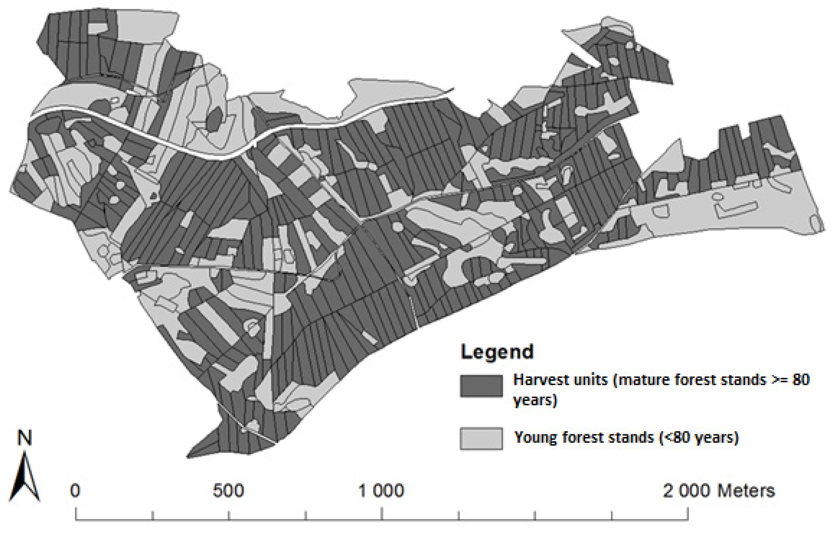
Figure 1.
The forest management area and edited harvest units.
Figure 1.
The forest management area and edited harvest units.
Real data on Norway spruce (standing volume) was used. To predict the growing stock, a growth model based on the Czech yield tables was used [
33].
In the next step, maps from the forest management plan were digitized to shapefiles and then analyzed in the ArcMap geographical information system. All parts of the FMA that were currently of cutting age, or would be within the next 30 years, were chosen. These parts of the FMA were then divided into potential cutting units by the editing tools in ArcMap. When editing these units, wind direction, slope, and existing logging roads were taken into account. On the other hand, it was important to consider also the legislative parameters for clear-cuts. This means primarily the maximum width, which equals two mean heights of the surrounding stand, and the maximum area of a clear-cut, which is one hectare.
It is not possible to determine the weights of the objective functions randomly and a proper way of subjective evaluation of the weights is sought. It is necessary to derive the weights in the proper manner because the importance of the functions is not equivalent. An expert opinion is needed to derive these weights. A questionnaire survey was used for this purpose. Weight values were obtained by questioning 21 experts from the field of forestry. This group consisted of experts representing obvious opinion polarities in the researched situation. There are experts who favor the economic benefits of forest management and, thus, the harvested volume maximization. However, there are also experts who prioritize the environmental aspects of forest management, favoring forest protection and growth preservation. Three expert groups were created by polarity in the researched situation for our purpose.
The opinions of the experts were obtained using questionnaire building on AHP. The task was to express their preference on a given scale for every pair of criteria (combinations of harvesting, protection and trees left standing) using their subjective point of view.
The collected data for each expert were transformed into the pairwise comparison matrix as defined by [
34], and, using this matrix, the criteria weights
for all experts
were calculated. At the same time, the consistency of Saaty’s matrix was tested. The consistency expresses the opinion consistency of the experts. If the consistency index reached a value over 0.1, the data was not included in the final weight determination. The final weights used in this model are then aggregations of the weights of each expert. The experts’ weights are aggregated considering the equal importance of each expert. The aggregation is performed via the following formulae:
Further, the different variants of harvest flow (α = 0.1, 0.2 and 0.3) have been calculated between periods and for a minimum size of the not harvested area of mature stands (λ = 0.05, 0.1 and 0.15, indicating 5.5, 11.0 or 16.5 hectares, respectively) for each period for each group.
Finally, the degree of fragmentation is calculated for each weighting combination. For this purpose, the so-called Shape Index can be used [
15,
35,
36].
The problem was solved using a branch and bound algorithm, which is a standard algorithm for solving mixed integer problems. The problem was formulated as a Gurobi LP format file and solved by Gurobi 5.5.0. A convergence of 0.01% was used.
3. Results
The stated problem was solved for five different weighting combinations. The sets of weights were divided into four groups: A–Production oriented, consisting of experts preferring criteria 1,
i.e., the maximization of the total cut; B–Not-harvested volume oriented, consisting of experts who prefer criteria 2,
i.e., minimization of the stand volume in the not-harvested stands; C–Perimeter oriented, consisting of experts who prefer criteria 3,
i.e., the minimization of the total perimeter of the not harvested area; and D–the neutral group, consisted of those experts with a neutral stance to the criteria. Additionally, the aggregate weights for all experts were used for calculations of a group called “All”. Five combinations were studied in total. For the particular weights and groups see
Table 1. The total harvested volume, the total perimeter of not harvested area, the total area of not harvested area and the total stand volume in not harvested area in the 1st period are presented (
Table 2).
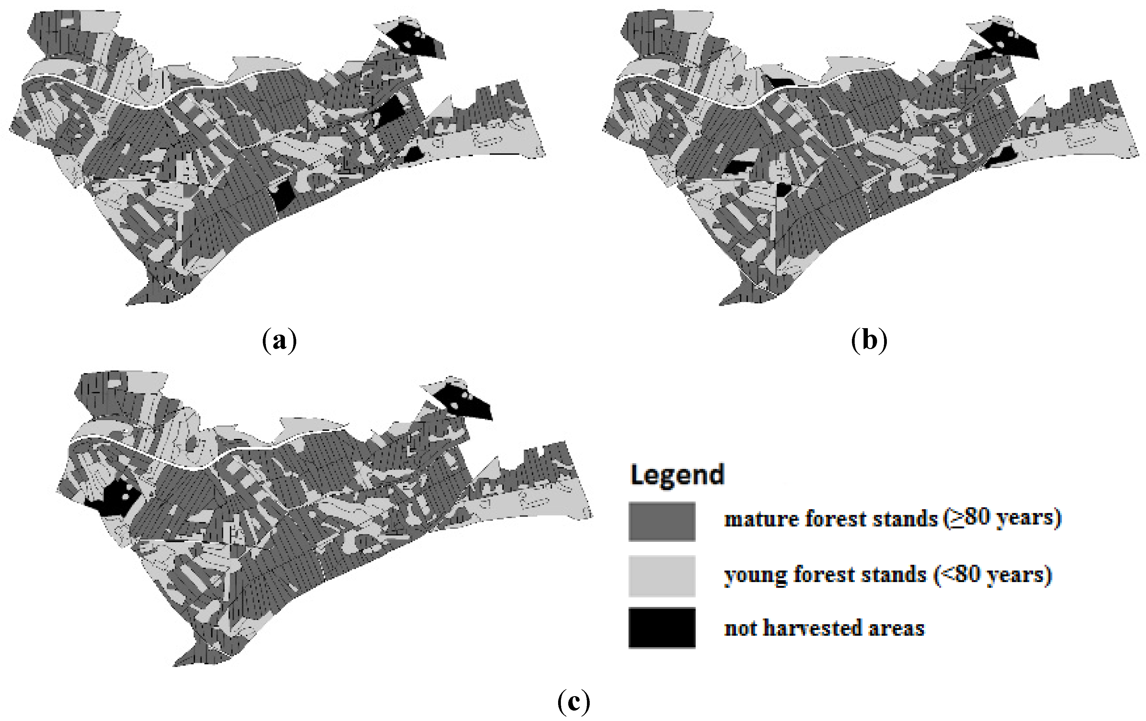
There are 45 graphical and numerical results altogether. For this reason, only the results for groups A, B and C are presented below as they represent extreme situations. The graphical results for different groups (A–C) for a not harvested area of 5% the total size and a harvest flow of 10% are presented (
Figure 2a–c). The graphical results support the achievement of the final shape indices of all groups. Most harvest units are aggregated for protection in the case of group C. By contrast, worse results of aggregation are provided by groups A and B. The differences between each group are easier to see in the cases of 10% and 15% not harvested area sizes (
Figure 3 and
Figure 4).
Table 1.
The different groups for the MultiCrit model.
Table 1.
The different groups for the MultiCrit model.
| Group | Weight 1 | Weight 2 | Weight 3 |
|---|
| A | 0.71 | 0.10 | 0.19 |
| B | 0.06 | 0.77 | 0.17 |
| C | 0.16 | 0.22 | 0.62 |
| All | 0.57 | 0.17 | 0.26 |
| Neutral | 0.43 | 0.22 | 0.35 |
Table 2.
The results of different variants of the MultiCrit model.
Table 2.
The results of different variants of the MultiCrit model.
| Group | The Minimum Size of Not Harvested Area (%) | The Harvest Flow Difference (%) | Total Harvested Volume (m3) | Total Perimeter of Not Harvested Area (m) | Total Area of Not Harvested Area (ha) | Total Stand Volume in Not Harvested Area in 1st Period (m3) |
|---|
| A | | 10 | 82,356 | 2463 | 5.66 | 1381 |
| 5 | 20 | 93,850 | 2463 | 5.66 | 1381 |
| | 30 | 95,958 | 2279 | 5.63 | 1318 |
| | 10 | 82,336 | 3169 | 11.19 | 8145 |
| 10 | 20 | 93,105 | 4373 | 11.19 | 4560 |
| | 30 | 94,760 | 4910 | 11.25 | 3685 |
| | 10 | 82,343 | 5625 | 16.81 | 10,846 |
| 15 | 20 | 91,643 | 7035 | 16.81 | 6577 |
| | 30 | 92,770 | 6934 | 16.82 | 6678 |
| B | | 10 | 81,956 | 2833 | 5.63 | 931 |
| 5 | 20 | 93,397 | 2833 | 5.63 | 931 |
| | 30 | 95,982 | 2833 | 5.63 | 931 |
| | 10 | 81,433 | 6259 | 11.25 | 2369 |
| 10 | 20 | 92,770 | 6259 | 11.25 | 2369 |
| | 30 | 94,931 | 3259 | 11.25 | 2369 |
| | 10 | 79,669 | 9773 | 16.87 | 4129 |
| 15 | 20 | 90,762 | 9773 | 16.87 | 4129 |
| | 30 | 93,241 | 9905 | 16.88 | 4093 |
| C | | 10 | 81,358 | 2034 | 5.65 | 1769 |
| 5 | 20 | 92,700 | 2034 | 5.65 | 1769 |
| | 30 | 95,390 | 2034 | 5.65 | 1769 |
| | 10 | 79,560 | 3929 | 11.19 | 4170 |
| 10 | 20 | 90,634 | 3929 | 11.19 | 4170 |
| | 30 | 93,253 | 4092 | 11.30 | 4152 |
| | 10 | 78,639 | 5814 | 16.81 | 7676 |
| 15 | 20 | 89,630 | 5814 | 16.81 | 7676 |
| | 30 | 90,113 | 6262 | 16.88 | 7024 |
| All | | 10 | 81,980 | 2234 | 5.61 | 1367 |
| 5 | 20 | 93,848 | 2463 | 5.66 | 1381 |
| | 30 | 95,951 | 2279 | 5.63 | 1318 |
| 10 | 10 | 81,936 | 4004 | 11.19 | 5198 |
| 20 | 92,679 | 4031 | 11.21 | 4878 |
| 30 | 94,292 | 4813 | 11.23 | 3310 |
| 15 | 10 | 81,266 | 5606 | 16.78 | 9547 |
| 20 | 90,121 | 5964 | 16.80 | 7484 |
| 30 | 91,551 | 6065 | 16.81 | 7317 |
| Neutral | | 10 | 81,944 | 2234 | 5.61 | 1367 |
| 5 | 20 | 93,425 | 2234 | 5.61 | 1367 |
| | 30 | 95,822 | 2234 | 5.61 | 1367 |
| | 10 | 81,225 | 3880 | 11.18 | 4978 |
| 10 | 20 | 92,499 | 3880 | 11.18 | 4978 |
| | 30 | 93,374 | 4172 | 11.24 | 4016 |
| | 10 | 79,243 | 6036 | 16.83 | 7676 |
| 15 | 20 | 89,930 | 5878 | 16.78 | 7596 |
| | 30 | 91,238 | 6687 | 16.85 | 6089 |
Figure 2.
Graphical results for different variants with 5% not harvested area and 10% harvest flow; (a) group A; (b) group B; (c) group C.
Figure 2.
Graphical results for different variants with 5% not harvested area and 10% harvest flow; (a) group A; (b) group B; (c) group C.
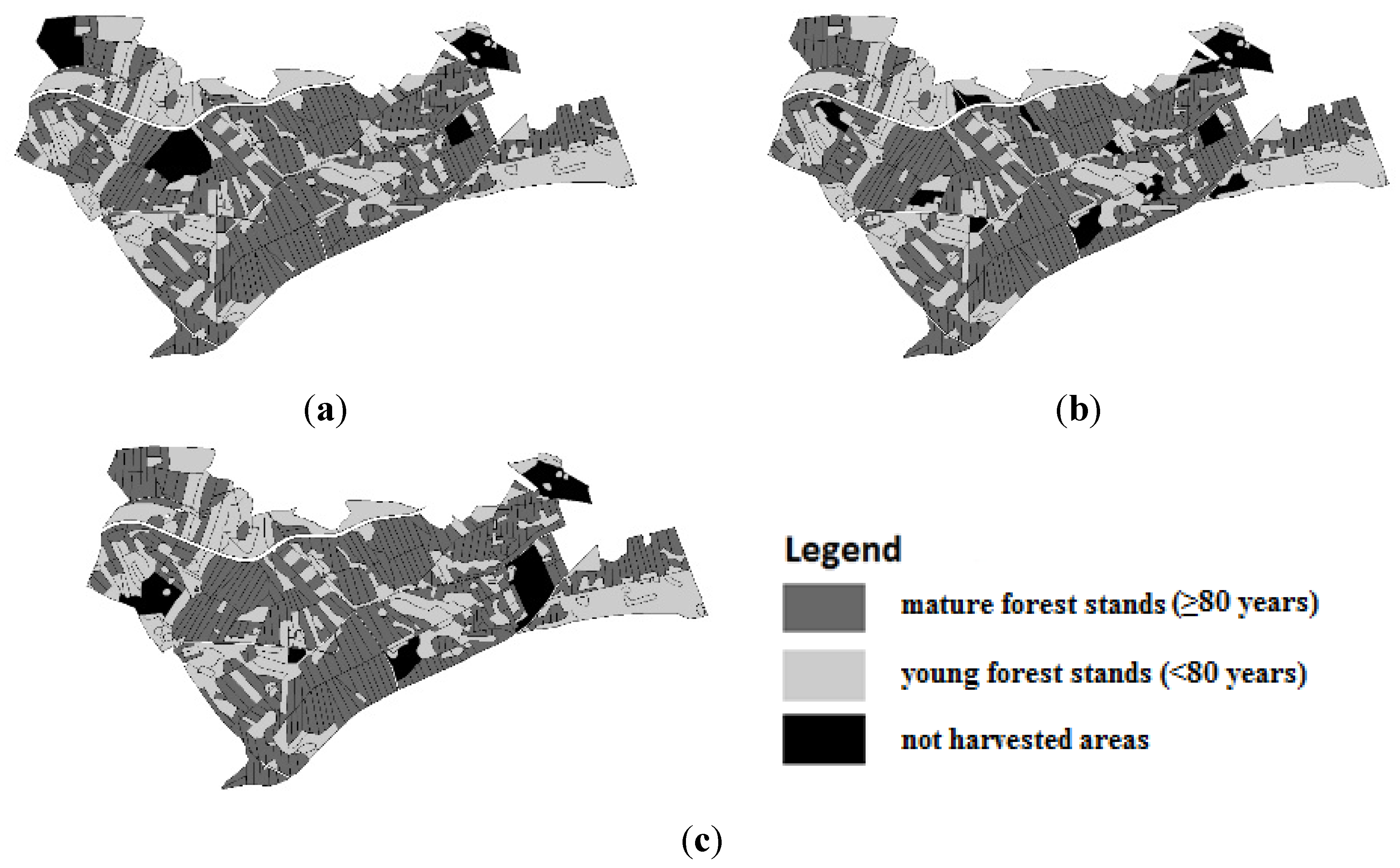
Figure 3.
Graphical results for different variants with 10% not harvested area and 10% harvest flow; (a) group A; (b) group B; (c) group C.
Figure 3.
Graphical results for different variants with 10% not harvested area and 10% harvest flow; (a) group A; (b) group B; (c) group C.
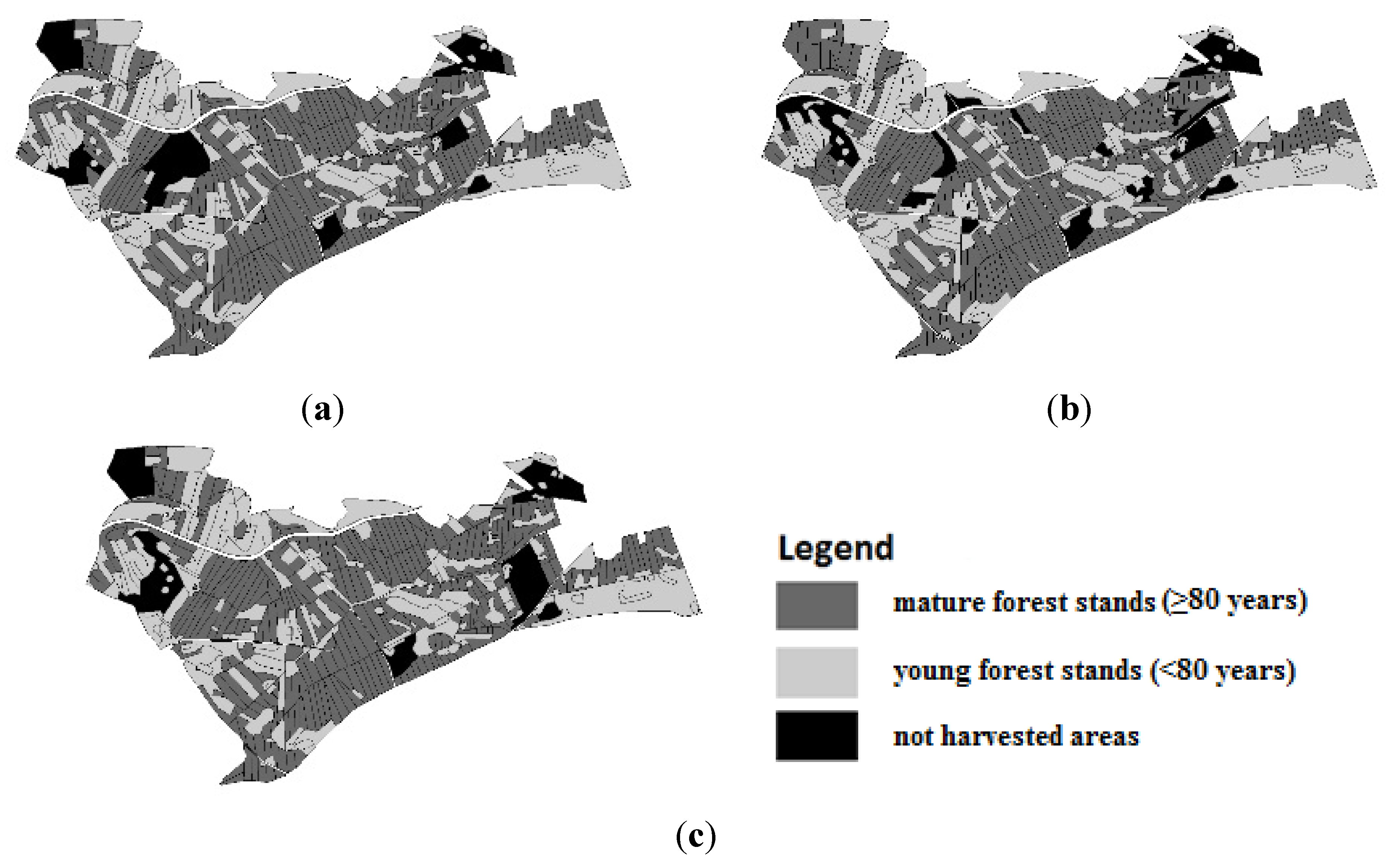
Figure 4.
Graphical results for different variants with 15% not harvested area and 10% harvest flow; (a) group A; (b) group B; (c) group C.
Figure 4.
Graphical results for different variants with 15% not harvested area and 10% harvest flow; (a) group A; (b) group B; (c) group C.
The results of Shape Index for different groups are presented in
Table 3. It is obvious that the best (
i.e., minimum) value of the Shape Index is in the case of group C which is the one with the highest weight put on the minimum outside perimeter objective function component. When comparing other groups, group A has smaller (better) resulting Shape Indices than do the variants of group B. However, group “Neutral” has better values of Shape index in a few variants than does group A.
Table 3.
The resulting Shape Index for groups A–C of the MultiCrit model according to the minimal size of the not harvested area and the harvest flow.
Table 3.
The resulting Shape Index for groups A–C of the MultiCrit model according to the minimal size of the not harvested area and the harvest flow.
| The Minimum Size of Not Harvested Area (%) | The Harvest Flow Difference (%) | Group |
|---|
| A | B | C |
|---|
| 5 | 10 | 2.92 | 3.37 | 2.42 |
| 20 | 2.92 | 3.37 | 2.42 |
| 30 | 2.71 | 3.37 | 2.42 |
| 10 | 2.67 | 5.27 | 3.31 |
| 10 | 20 | 3.69 | 5.27 | 3.31 |
| 30 | 4.13 | 5.27 | 3.43 |
| 15 | 10 | 3.87 | 6.71 | 4.00 |
| 20 | 4.84 | 6.71 | 4.00 |
| 30 | 4.77 | 6.80 | 4.30 |
All potential harvest units are not managed (suggested for harvesting or not-harvesting) over the planning horizon because of adjacency constraints. There are 8.10, 6.13 and 5.87 hectares of non-managed forests for three harvest flow differences in the case of the simple harvest scheduling problem presented below. The greater is the harvest flow difference, the smaller is the non-managed area. The same dependence is obvious in the case of all variants of groups of the multiple-use harvest scheduling problem (
Table 2). However, the absolute values of this are much higher (from 11.77 hectares to 33.44 hectares) than in the case of the multiple-use forestry scheduling problem.
In the MaxHar model there is a higher total harvested volume over the planning horizon, of course, because there is not a not harvested area demand to compare with the MultiCrit model. Although the results of the MaxHar model are rather obvious, they are presented anyway to demonstrate the difference when compared with the other models. The differences range from 26.8% to 32.7% in the case of 10% harvest flow difference, from 11.3% to 16.6% in the case of 20% harvest flow difference and from 9.1% to 16.1% in the case of 30% harvest flow difference for all groups.
4. Discussion
A multiple-use harvest scheduling model was presented. The results show that the spatial pattern and other spatial demands affect the harvest possibilities. One can see in the example of the MaxHar model that, in the case of only the maximization goal, some harvest units are non-managed because of the adjacency constraints. The primal hypothesis could be that this part of the non-managed forest can be protected without an effect on the total harvested volume over the planning horizon. However, the presented results do not confirm this assumption as it was shown. The spatial demand for a continuous area of mature forest stands has a large effect on the adjacency because inclusion of the consideration of spatial relationships in long-term planning will increase the complexity of the task [
15]. However, the purpose of forest planning and the harvest scheduling model is to suggest management alternatives and information about management consequences and to assist with decision making [
37].
The total harvested volume over the planning horizon in the
MultiCrit model was higher with group A than groups B and C. This result was predictable and is consistent with the results by [
15,
16]. The authors [
16] created a harvest scheduling model for net present value (NPV) maximization and perimeter minimization. They tested five weighting combinations. The resulting net present value was in the case with NPV weight = 1 − e (e is very small number) about 5.4% higher than in the case with NPV weight = 0.1.
The other study [
15] used a similar approach. However, the authors showed that the total harvested amount through 10 periods was almost the same for all weight combinations except for the last weight combination which had a perimeter weight = 1 − e (e is very small number). The authors created their scheduling models in which each forest stand is presented by one variable and use only two criteria as NPV maximization and perimeter minimization. By contrast the previous case presented the
MultiCrit model calculated with
a priori defined harvest units with a strict defined size which resulted in many units within one forest stand. This means that spatial structure is more complicated when a forest stand approach is used as demonstrated in the presented model.
The presented model shows that the total harvested volume and non-managed area over the planning horizon is dependent on the harvest flow difference (
Table 2). If the difference is greater, the non-managed area is smaller and the total harvested volume is greater. However, the difference between the non-managed area and the total harvested volume is greater for the 10% and 20% harvest flow differences compared to the 20% and 30% harvest flow difference. It seems that the higher harvest flow difference can produce a higher scheduled harvest, but the increases can be ineffective beyond a certain point. This point can be considered a very important component of the decision process, especially in the case of non-regulated forests, and it is to be investigated in our future research.
The groups were derived using an anonymous questionnaire that was distributed among forest experts. For this reason, the groups reflect the real opinions of foresters more so than in the case of artificially set weighting combinations by scientists [
15,
16]. However, the presented approach shows the problems that can arise from using Saaty’s methods for more than three criteria in real-life scheduling problems, such as the need for a questionnaire with very detailed descriptions, inconsistencies,
etc.Our results show that foresters can manage forests for production while other ecosystem requirements are met. The presented scheduling model, considering both economic and ecological goals, can help forest planners and managers understand the spatial pattern of harvest units needed to ensure that an adequate protected area is set aside, like with the spatial planning model by [
20]. Furthermore, computing the trade-offs between timber revenues and aspects of biodiversity protection is useful for policy makers and forest owners or managers who have different types of forest certifications.
It is possible that forester cannot adhere to the optimal plan of harvesting for some unexpected reasons. Even then, the proposed harvesting scheme can be applied in different ways. The results of individual variants show that there are certain harvest units appearing with the same result for each variant. Either there are those units that are supposed to be harvested every time regardless of the variant, or, similarly, there are such units that are supposed to be not harvested no matter what variant was computed. These individual units are included in every variant due to their suitable ratio of attributes (standing volume, shape, and position in FMA, etc.). It is possible to mark these units as “recommendable” for harvesting (or not harvesting) regardless of which optimal plan was used. If forester cannot fully keep the optimal plan then at least the recommendable units should be harvested to approach the optimal solution.
The proposed solution is presented within the forest management in the Czech Republic, but it could be implemented in any forest management practice in central Europe. It shows how to maximize the amount of harvested wood while ensuring the conditions for forest species existence are also preserved. The model of mathematical programming is generally suitable for all forest management areas of a similar size. Once having data describing any forest management area, it is then not very complicated or time-consuming to provide the compromise solution and, thus, a better plan of forest harvesting as a service for whoever desires to improve the effectiveness of forest harvesting.
The initial idea was to develop a harvest scheduling model applied in the managed forests of central Europe. The presented scheduling model is of course inspired by other authors and lacks important factors such as dead wood, large trees dimensions etc. However, it was confirmed that a compromise solution from both forest management and nature conservation could be achieved using the presented harvest scheduling approach.
It is possible to assume that the protected area would not be static in the long-term planning and would change position over time as well as include other aspects of biodiversity. A solution to this problem will be the next stage of our forest harvesting research.


