Article

Climate Change Will Reduce the Carbon Use Efficiency of Terrestrial Ecosystems on the Qinghai-Tibet Plateau: An Analysis Based on Multiple Models

1
Institute of International Rivers and Eco-Security, Yunnan University, Kunming 650500, China
2
State Key Laboratory of Urban and Regional Ecology, Research Center for Eco-Environmental Sciences, Chinese Academy of Sciences, Beijing 100085, China
3
Department of Biology Sciences, Institute of Environmental Sciences, University of Quebec at Montreal, Montréal, QC H2L 2C4, Canada
*
Author to whom correspondence should be addressed.
Forests 2021, 12(1), 12; https://doi.org/10.3390/f12010012
Submission received: 12 November 2020 / Revised: 11 December 2020 / Accepted: 22 December 2020 / Published: 24 December 2020
(This article belongs to the Section Forest Ecology and Management)

Abstract

:
The carbon use efficiency (CUE) of ecosystems, expressed as the ratio of net primary production (NPP) and gross primary production (GPP), is extremely sensitive to climate change and has a great effect on the carbon cycles of terrestrial ecosystems. Climate change leads to changes in vegetation, resulting in different CUE values, especially on the Qinghai-Tibet Plateau, one of the most climate-sensitive regions in the world. However, the change trend and the intrinsic mechanism of climate effects on CUE in the future climate change scenario are not clear in this region. Based on the scheme of the coupled model intercomparison project (CMIP6), we analyze the simulation results of the five models of the scenario model intercomparison project (ScenarioMIP) under three different typical future climate scenarios, including SSP1-2.6, SSP3-7.0 and SSP5-8.5, on the Qinghai-Tibet Plateau in 2015–2100 with methods of model-averaging to average the long-term forecast of the five several well-known forecast models for three alternative climate scenarios with three radiative forcing levels to discuss the CUE changes and a structural equations modeling (SEM) approach to examine how the trends in GPP, NPP, and CUE related to different climate factors. The results show that (1) GPP and NPP demonstrated an upward trend in a long time series of 86 years, and the upward trend became increasingly substantial with the increase in radiation forcing; (2) the ecosystem CUE of the Qinghai-Tibet Plateau will decrease in the long time series in the future, and it shows a substantial decreasing trend with the increase in radiation forcing; and (3) the dominant climate factor affecting CUE is temperature of the factors included in these models, which affects CUE mainly through GPP and NPP to produce indirect effects. Temperature has a higher comprehensive effect on CUE than precipitation and CO2, which are negative effects on CUE on an annual scale. Our finding that the CUE decreases in the future suggests that we must pay more attention to the vegetation and CUE changes, which will produce great effects on the regional carbon dynamics and balance.

1. Introduction

According to the Fifth Assessment Report of the Intergovernmental Panel on Climate Change (IPCC), global warming and greenhouse gas increases are the main characteristics of current and future global climate change [1], which affects the dynamics of terrestrial ecosystem carbon cycles. As two important indicators of vegetation productivity, gross primary production (GPP) and net primary production (NPP) represent the carbon gain abilities of ecosystems [2]. The ratio of NPP and GPP, termed the carbon use efficiency (CUE) of ecosystems [3,4,5], determines the carbon sink function, carbon cycle and turnover rate of vegetation [6], indicating the efficiency of the ecosystem in absorbing carbon from the atmosphere into a terrestrial biomass. CUE is considered to be an important parameter for formation of the ecosystem carbon pool [7], reflecting the ability to transfer carbon from the atmosphere to a potential carbon sink and determining the carbon distribution of NPP and respiration [8], which are two basic components of GPP. In addition, as an indispensable parameter in the ecosystem model, a slight modification of the CUE value may lead to drastic changes in the model’s prediction ability [7], especially when the research scale is enlarged from a landscape to a terrestrial ecosystem.
Recent CUE research has focused on the change characteristics of CUE in the past decade on a regional or global scale, and this research was mainly based on remote sensing data, flux observation data and model simulation evaluations [9,10,11,12]. Some studies showed that the CUE value of terrestrial ecosystems is a relatively constant, ranging from 0.47–0.50 [13,14,15]. There are also some studies showing that the CUE changes with changes in the environment [16,17]. Increasing evidence shows that CUE will be affected by environmental factors, including vegetation type, ecosystem type, climate conditions, nitrogen deposition, management conditions, site fertility and stand age, and changes dynamically at different time scales [4,17,18,19,20,21]. For example, De Lucia, et al. [17] found that the CUE ranged from 0.23–0.80 and increased with increasing forest age. Based on MODIS data and NPP estimation data from a forest field survey, Kwon and Larsen [22] found that CUE decreases with increasing temperature and precipitation but increases with increasing latitude and altitude, which indicated that CUE is a substantial variable. Chen et al. [6] found that there is a linear relationship between the average annual temperature and CUE. The increase in temperature will lead to an increase in respiratory enzyme activity and the enhancement of plant respiration [5]. In future long-term series, there are few studies on change predictions of CUE. In the context of future climate change, the response of CUE to climate and the resulting changes remain controversial.
With model development being increasingly improved to be more accurate, research using model data to analyze CUE is increasing. In previous studies, there is much research on the analysis of CUE characteristics by using eddy flux data and remote sensing data. The eddy covariance method is being applied by the global change community on the increasingly longer time scales [23,24]. The eddy flux data and remote sensing data can be processed using a variety of methods in confluence with ground and other data sources to analyze and verify the value and trend of CUE. In addition, some studies have proposed that the conclusions drawn from a single model dataset are more sensitive to systematic bias and errors, which makes it very important to use multiple data sets for research [25,26]. Moreover, using model forecast models and averaging the results can result in more reliable results by balancing any biases in any single model [25,26,27,28,29]. The Qinghai-Tibet Plateau is very sensitive to climate change; however, there is no conclusion on the future response of CUE to climate change in this region. Therefore, the interest is obtaining reliable forecasts that can indicate the impacts of possible future climate scenarios on this region. It is of great value to use model-averaging to predict the future change in CUE in the Qinghai-Tibet Plateau for the study of the regional carbon cycle in the context of climate change.
Based on the three typical climate scenarios of the Scenario Model Intercomparison Project (ScenarioMIP) of the Coupled Model Intercomparison Project Phase 6 (CMIP6), this paper studies the interannual variation characteristics of CUE in the Qinghai-Tibet Plateau under the background of future climate change by using the model-averaging method. The objectives of this study are (1) to quantify the change characteristics of GPP, NPP and CUE; (2) to analyze the influencing factors of CUE changes in the five models under three typical scenarios; and (3) to explore the impact mechanism of key climate factors on CUE in the region. Accurately predicting the change trends of future CUE has a certain reference value for assessment of the regional carbon budget in the context of climate change in the Qinghai-Tibet Plateau, which will provide a case study that can inform the development of carbon management measures in response to climate change and provide insight into regional carbon cycle change in the Qinghai-Tibet Plateau.

2. Data and Methods

2.1. Study Area

The Qinghai-Tibet Plateau is located at 26°00′12″ N—39°46′50″ N, 73°18′52″ E—104°46′59″ E [30], which is located from the Pamirs Plateau in the west to the Hengduan Mountains in the east, the southern margin of the Himalayas in the south, and the Kunlun-Qilian Mountains in the north. The Qinghai-Tibet Plateau is approximately 2945 km long from east to west and 1532 km wide from south to north, with an area of approximately 2.57 × 10⁶ km2, accounting for 26.8% of China’s total land area. The Qinghai-Tibet Plateau includes the Tibet Autonomous Region and parts of the Qinghai Province, Xinjiang Uygur Autonomous Region, Gansu Province, Sichuan Province and Yunnan Province. The Qinghai-Tibet Plateau has the highest altitude and largest area, and it is the most-recently formed plateau in the world, which is a large tectonic geomorphic unit. The terrain is inclined from northwest to southeast. In the Qinghai-Tibet Plateau, it is cold and dry in the northwest and warm and humid in the southeast. The dry and wet seasons are distinct, and the annual and daily temperature ranges are large. The vegetation is characterized by alpine desert, alpine meadow and grassland landscapes, and the soil is mainly composed of coarse textures, thin soil layers and poorly developed alpine meadow soil and alpine cold desert soil in the Qinghai-Tibet Plateau.

2.2. Dataset Descriptions and Validation

The primary data are derived from the database of the Program for Climate Model Diagnosis and Intercomparison (PCMDI) (https://pcmdi.llnl.gov/CMIP6/). PCMDI data were distributed by the IPCC Data Statistics Center. After all simulation results and other results were counted, the PCMDI database was established and shared free of charge. The model results of CMIP6 has been verified in the global scale, and it is a common practice to use these models to analyze the results [31,32,33,34,35,36,37,38]. Here we used model-averaging to increase the reliability of the forecasts and interpretation of factors that impact the model-averaged forecast. Considering the data integrity of relevant statistics, such as research purposes and scenarios, we selected CESM2, CESM2 WACCM, EC-EARTH3-VEG, MPI-ESM1-2-HR, and BCC-CSM2-MR of scenario MIP, one of the subplans of CMIP6 [39,40] (Table 1), based on three radiative forcing levels, SSP1-2.6, SSP3-7.0, and SSP5-8.5 varying the radiative forcing to ~2.6 W/m2, ~7.0 W/m2, and ~8.5 W/m2, respectively; we chose monthly GPP, NPP, precipitation and temperature predicted by corresponding models for analysis. The data are in NetCDF format with a nominal resolution of 100 km that covers the globe. Due to the lack of CO2 concentration data in the corresponding model, the future long-term series CO2 prediction data come from the CO2 concentration data in the 21st century scenario designed by Riahi et al. [41].
For model validation, except comparing the results of other publish model, we also chose Moderate Resolution Imaging Spectroradiometer (MODIS) data (GPP from MYD17A2H and NPP from MYD17A3H, https://lpdaacsvc.cr.usgs.gov/appeears/products) as one of the bases to discuss and verify the results of multi model calculation. The data of annual NPP and GPP accumulated 8 day of data from 2000 to 2010 were obtained by MODIS. We converted the 8-day GPP data into annual GPP data. We added up to all 8-day GPP data to obtain the annual GPP data. For each year, we calculate the spatial average value to obtain the average level of this index after eliminating the outliers in the Qinghai-Tibet plateau. Finally, the spatial value of each year’s CUE is obtained by calculating the ratio of annual NPP and GPP of each year from MODIS from 2000 to 2010 for the validation with model-averaging of the same period each Year).

2.3. Variable Time Series and Trend Analysis

The corresponding data of the five models of the Qinghai-Tibet Plateau from 2015 to 2100 are extracted to calculate the CUE, GPP, NPP, mean annual precipitation (MAP) (Figure A2 in Appendix A), mean annual temperature (MAT) (Figure A1) and CO2 concentration (Figure A3). Based on the monthly data of the corresponding model range of the Qinghai-Tibet Plateau in the historical period (1951–2014), the annual average values of CUE, GPP, NPP, MAP and MAT in this period are calculated. The deviation values of the future period relative to the historical period among different model are analyzed to forecast the future climate change in the Qinghai-Tibet Plateau terrestrial ecosystem and the change trends of GPP, NPP and CUE under future climate scenarios in a long time series. We used the commonly used climate tendency rate to examine time gradient [42], where this is defined by:
Yi = a0 + ati,
where Yi is dependent variable for each year (ith year), a is the slope (that is tendency rate, indicating the annual change trend of change factors) and ti is the independent variable that means the time series (ith year) and the a0 is the intercept. In this paper, the change trend of the long time series of CUE, GPP, NPP, MAP, MAT, and CO2 concentrations in the Qinghai-Tibet Plateau is expressed by the tendency rate. If p-value is less than 0.05, it means the original hypothesis can be rejected.

2.4. Structural Equation Model

Structural equation modeling (SEM) is a method to establish, estimate and test causality model. The model contains both observable and latent variables. SEM can replace multiple regression, path analysis, factor analysis, covariance analysis and other methods to clearly indicate the effect of observable variables and latent variables [43]. This method assumes that there is a causal relationship between variables, and latent variables are usually formed by a linear combination of some observable variables. SEM is composed of a measurement model and structural model. The measurement model focus on how well the indicators load on the latent factors. The structural model represents the causal relationship between observable variables and latent variables, which focus on how well observable variables predict and explain latent variables and is generally expressed in the form of a path diagram. The general expression of the SEM is described as follows:
X = ΛXξ + δ,
Y = ΛYη + ε,
η = βη + Γξ + ζ
Formulas (2) and (3) are measurement models, where X is the measurement variable matrix of potential independent variable ξ, ΛX is the measurement coefficient matrix, and δ is the residual matrix of measurement Equation (2). Y is the measurement variable matrix of potential dependent variable η, ΛY is the measurement coefficient matrix, and ε is the residual matrix of measurement Equation (3). Formula (4) is the structural model in the SEM, where ξ is the potential independent variable matrix, η is the potential dependent variable matrix, Γ is the path coefficient matrix, which is affected by the potential independent variable matrix ξ that affects the potential dependent variable matrix η, β is the path coefficient matrix that represents the mutual influence between the constituent factors of the potential dependent variable matrix η, and ζ is the residual matrix of Equation (4). Based on the analysis of the correlation between the CUE and GPP, NPP, MAP, MAT, and CO2 concentrations in the Qinghai-Tibet Plateau ecosystem, the SEM is used to explain the relationship between the CUE and the other variables under three future climate scenarios.
To evaluate the complex relationship between variables, we used the SEM to test the direct and indirect effects of each variable on CUE. We design a hypothetical model in which the observed variables MAT, MAP and CO2 can directly affect GPP, NPP, and CUE. According to the fitting index and Akaike information criterion (AIC), the SEM with the lowest AIC value was selected [44]. The standardized coefficients were used to explain the direct effects of different paths [45]. We added standardized direct effects of all given exogenous variables to calculate their total impact on CUE [46]. The SEMs were fitted by using the lavaan package (Version 0.6-6, Ghent, Belgium) [47]. All analyses were performed in R (Version 3.5.1, Vienna, Austria.) [48].

3. Results

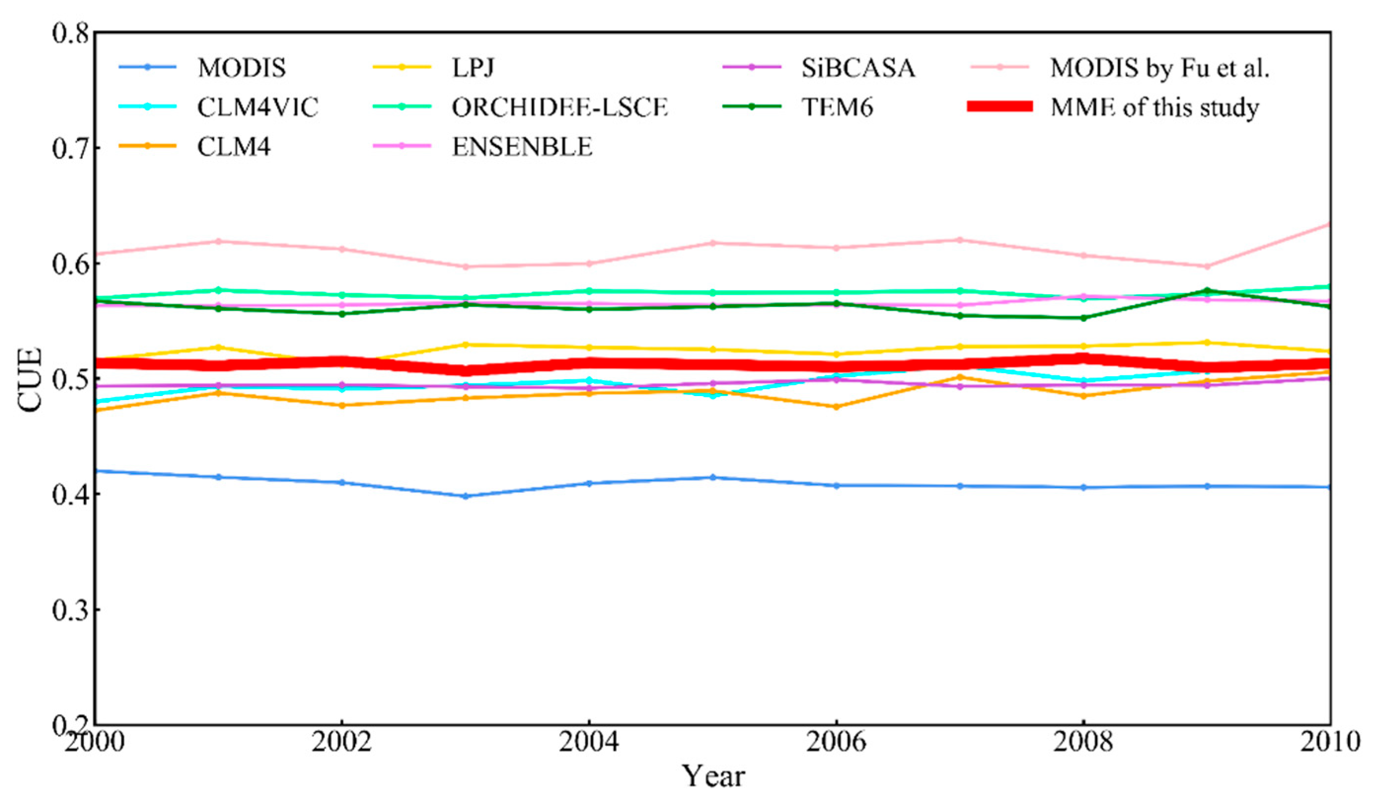
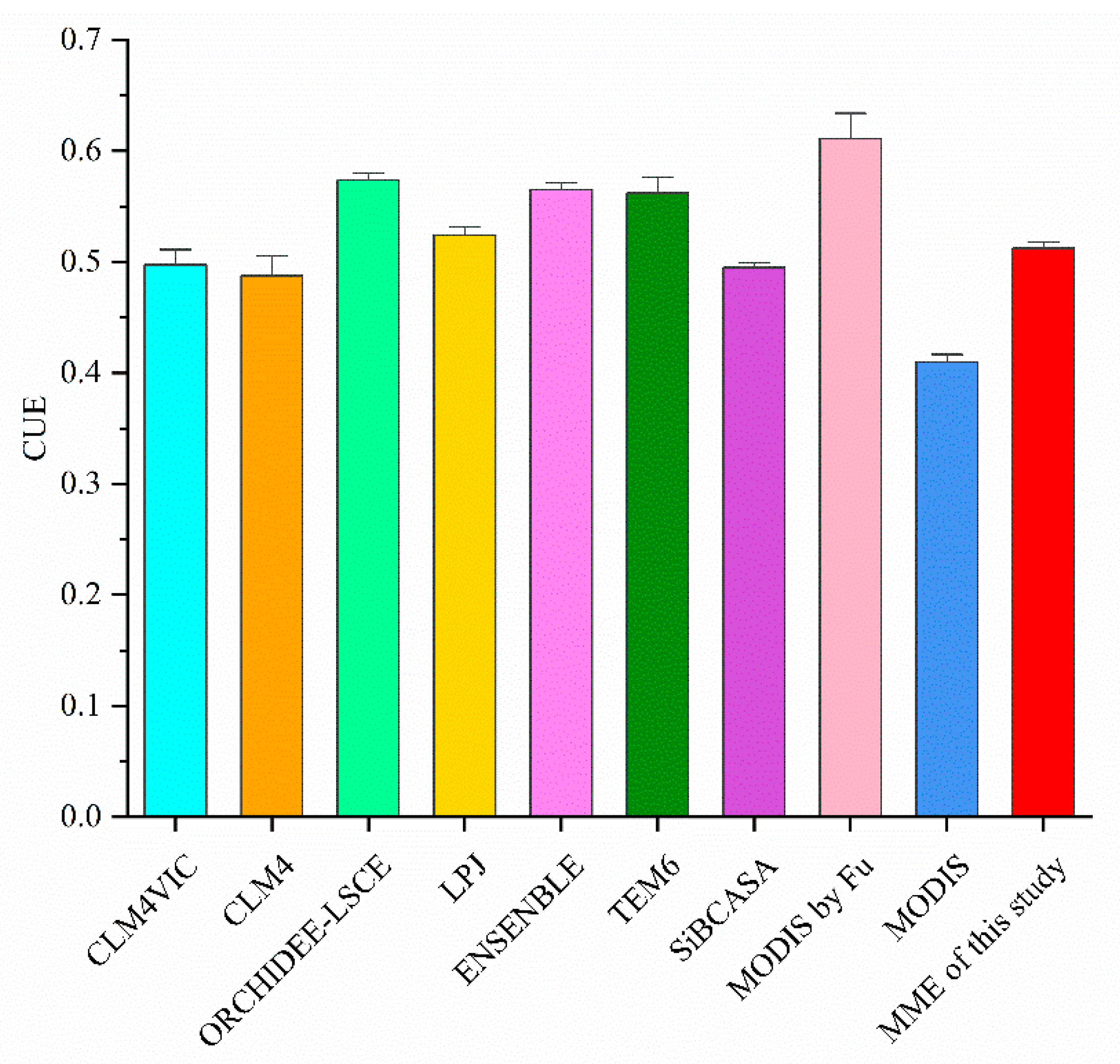
3.1. Cross-Validation of Model-Averaging with MODIS and Other Studies

The CUE values of this study are highly consistent with the results of other studies (Figure A4). We have done a lot of work, looking for and analyzing various kinds of data sources of other studies to conduct interactive verification of CUE during the historical period of the Qinghai-Tibet Plateau from 2000 to 2010. Compared with MODIS data and other research results, we found that there are consistency and differences. From 2000 to 2010, compared with MODIS result of 0.41, the mean value of CUE from the model-averaging is 0.51, which has some differences on the Qinghai-Tibet Plateau. However, the CUE obtained from the model-averaging in this study are highly consistent with the CUE of models calculated by Luo et al. [49] on the Qinghai-Tibet Plateau. The CUE is between 0.507–0.517 by using model-averaging in the Tibetan Plateau (Figure A4), and that calculated by Luo et al. is between 0.45–0.7 relatively, of which the results of LPJ model are the most consistent with results of ours. The mean annual CUE of LPJ model is 0.52, and that of CUE in this study is 0.51 (Figure A5). The CUE calculated by this study is among the results of CLM4VIC, CLM4, ORCHIDEE-LSCE, LPJ and SiBCASA model (Figure A4). Fu et al. [11] calculated the CUE by using (MODIS data that get the maximum CUE values. There are some differences between the results of the MODIS and models, thus the reliability of MODIS results also needs to be verified.

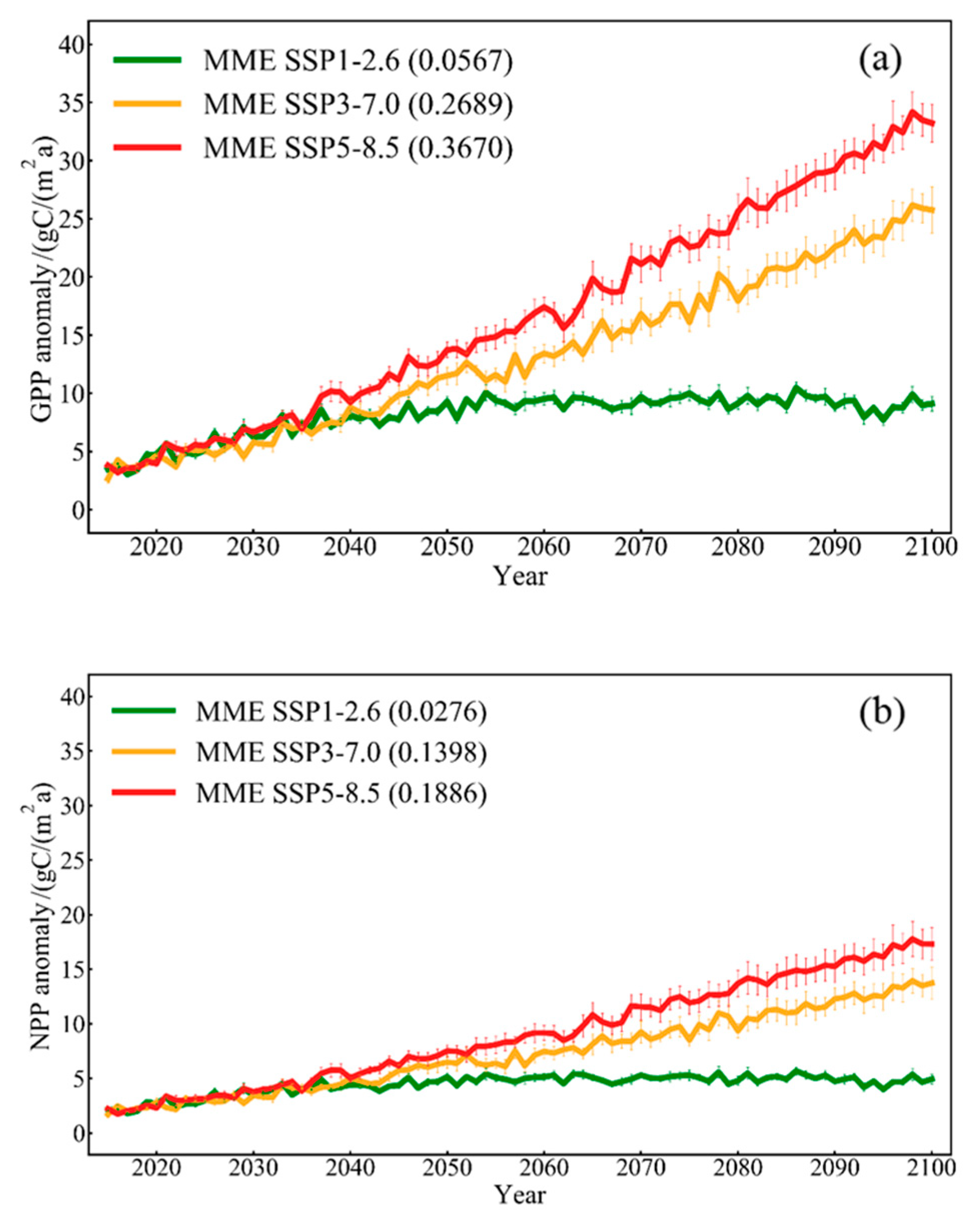
3.2. Change Trend Characteristics of GPP, NPP and CUE

Compared with the reference period of 1951–2014, the mean GPP deviations for the three climate scenarios showed an increasing trend in the future long time series (Figure 1a). From 2015 to 2100, under the scenarios of SSP1-2.6, SSP3-7.0 and SSP5-8.5, the multi-year mean GPP is 31.38–38.82, 30.99–54.52 and 31.57–62.53 gCm−2a−1, respectively, and compared with the historical period, the annual average deviations of GPP are 3.03–10.48, 2.65–26.17 and 3.21–34.17 gCm−2a−1, respectively. In future long-term series (2015–2100), GPP increases with increasing radiation forcing. Under the three scenarios on the interannual scale, the tendency rates of GPP are 0.0567, 0.2689 and 0.3670 gCm−2a−1 (Table A1), which reach a substantial level. With the increase in radiation forcing, the increasing trend becomes increasingly larger.
The deviation values of NPP in different scenarios relative to historical periods are consistent with GPP in future long time series (Figure 1b). In 2015–2100, under the scenarios of SSP1-2.6, SSP3-7.0 and SSP5-8.5, the annual mean NPP values are 16.82–20.72, 16.73–28.98 and 16.76–32.81 gCm−2a−1, respectively. The annual average deviations of NPP are between 1.78–5.68, 1.69–13.94 and 1.73–17.77 gCm−2a−1. At the interannual scale, the NPP propensity rates of the three scenarios are 0.0276, 0.1398 and 0.1886 gCm−2a−1 (Table A1), reaching substantial levels, and the increasing trend is obvious with the increase in radiation forcing. Under the same scenario, the tendency rate of GPP is higher than that of NPP, which indicates that the growth rate of GPP is higher than that of NPP in each scenario. Comparing GPP and NPP under the same scenario, the NPP value is close to half of the GPP value, i.e., the CUE (NPP/GPP) value is approximately 0.5.
From 2015 to 2100, the CUE values of the SSP1-2.6, SSP3-7.0 and SSP5-8.5 scenarios ranged from 0.502 to 0.520, 0.498 to 0.522 and 0.497 to 0.520, respectively (Figure 2). The results reveal that CUE shows different degrees of decline under the scenarios of SSP1-2.6, SSP3-7.0 and SSP5-8.5 in the future long-term series in the Qinghai-Tibet Plateau. The tendency rates of CUE in the SSP1-2.6, SSP3-7.0 and SSP5-8.5 scenarios are −3.50 × 10⁻⁵, −1.12 × 10⁻⁴ and −1.76 × 10⁻⁴, respectively (Table A1). This result indicates that with the increase in radiation forcing, the downward trend of CUE in the long-term series increases in turn, and the stronger the radiation is, the smaller the value of CUE. Under the same scenario, the tendency rate is higher than that of NPP, and with the increase in radiation forcing, the rate of increase in GPP is higher than that of NPP, which also explains the change in CUE from the other side.

3.3. Correlation between CUE and Climate Change Factors

GPP, NPP and CUE under three future climate scenarios representing different radiative forcings have substantial correlations with the climate variables MAT, MAP and CO2 concentration (Figure 3). GPP and NPP are highly positively correlated with MAT and CO2 concentration, respectively, and there is little substantial difference among scenarios. The positive correlation between MAP and GPP and NPP is slightly lower in the low radiation forcing scenario than in the medium and high radiation forcing scenarios. CUE and MAT, MAP, and CO2 concentrations show different degrees of negative correlation under the three scenarios. CUE has a low negative correlation with MAT and CO2 concentration under the SSP1-2.6 scenario (Figure 3a), increasing under the SSP3-7.0 scenario (Figure 3b), and has the highest negative correlation with them under the SSP5-8.5 scenario (Figure 3c). Thus, the negative correlation between CUE and MAT and CO2 concentration increases with the increase in radiative forcing; that is, the higher the temperature and CO2 concentration are, the CUE shows an increasingly obvious decreasing trend. The negative correlation between CUE and MAP is slightly weaker than that between CUE and MAT and CO2 concentration, especially in the low radiation forcing scenario. Likewise, the negative correlation between CUE and MAP becomes increasingly substantial with increasing radiative forcing.

3.4. Control Mechanisms of CUE Changes under Three Scenarios

The results from the SEM explain the possible influencing paths of CUE changes. Under the scenarios of SSP1-2.6, SSP3-7.0 and SSP5-8.5, MAP, MAT and CO2 concentrations have little direct impact on CUE, but they have indirect impacts on CUE through GPP and NPP (Figure 4). Under the three scenarios, the direct path coefficient of MAT to GPP is positive and the largest compared with MAP and CO2 concentration; thus, MAT has the greatest direct impact on GPP compared with MAP and CO2 concentration. Similarly, MAT has a greater direct impact on NPP than MAP and CO2 concentration, but it has a negative effect on NPP under the SSP1-2.6 scenario and SSP3-7.0 scenario and a positive effect under the SSP5-8.5 scenario.
Under the SSP1-2.6 scenario, the direct path coefficient of MAT to CUE is -0.005, and the indirect path coefficient of MAT to CUE through GPP and NPP is −0.293. Thus, the total coefficient between MAT and CUE is −0.298 (Table A2). The direct effects of MAP and CO2 concentration on CUE are negligible, and their indirect path coefficients are 5.14 × 10⁻⁵ and 6.8 × 10⁻⁶, respectively. Thus, the comprehensive effect of MAT on CUE is far greater than that of MAP and CO2 concentration, and MAT has a negative effect on CUE, while MAP and CO2 concentration have a weak positive effect on CUE.
Similarly, under the SSP3-7.0 and SSP5-8.5 scenarios, the direct path coefficients of MAT to CUE are −0.005 and −0.006, respectively, and the total coefficients are −0.005 and −0.004, respectively. Under these two scenarios, the comprehensive path coefficients of MAP to CUE are 1.9 × 10⁻⁴ and 3.4 × 10⁻⁵, respectively. The comprehensive path coefficients of CO2 concentration on CUE are −2 × 10⁻⁵ and −6 × 10⁻⁵ (Table A2). Thus, under the SSP3-7.0 and SSP5-8.5 scenarios, the comprehensive impact of MAT on CUE is also much greater than that of MAP and CO2 concentration. The MAT still has a negative effect on CUE, and MAP has a very weak positive effect on CUE. However, the difference is that the comprehensive effect of CO2 concentration on CUE changes from a weak positive effect to a weak negative effect after changing from the low radiation forcing scenario to the medium and high radiation scenarios. In Figure 4, R2 reflects the comprehensive decisive effect of GPP, NPP, MAT, MAP and CO2 on CUE [50]. It is found that climate variables play an increasing strong role in controlling CUE by adjusting GPP and NPP under the conditions of radiation forcing increasing.

4. Discussion

4.1. Importance of the Model-Averaging Method

In this research, we study the interannual variation characteristics of CUE in the Qinghai-Tibet Plateau based on the three typical climate scenarios of the ScenarioMIP of CMIP6 by using model-averaging, and we forecast that the CUE of the Qinghai-Tibet Plateau ecosystem will increase under future climate scenarios. In addition, we explore the mechanism of key climate factors impacting CUE in the region and reveal that temperature has a more dominant effect on CUE than precipitation and CO2 in the Qinghai-Tibet Plateau.
We try to use the model-averaging to get more reliable results. One of the main reasons for using the model-averaging is that model-averaging tends to reduce any deviation of any single model. Another reason for using it is that the model-averaging result are consistent with the results calculated by other alternative models, which leads to greater confidence in the forecasts of model-averaging. In addition, compared with results drawn by single point observations, model-averaging forecast can effectively reduce the uncertainty on the continuous macro spatial scale. Compared with remote sensing data analysis, the existing research shows that the CUE analysis results of remote sensing are consistent with the simulation results of the ecosystem process model [23]. By comparing the trend of climate change with existing studies, the results of model-averaging are in good agreement with previous studies [26], which further brings the confidence of the results of model-averaging research.

4.2. Comparison of the Change Trend of CUE

As an important indicator of the carbon cycle in terrestrial ecosystems, CUE is still controversial. The prediction results of CUE in the future climate scenarios show that there is a slight downward trend in a long time series in the Tibetan Plateau from 2015 to 2100, and the decreasing degree gradually increases with the increase in radiation forcing. The same results can be found in the research of Yuan et al. [51], which shows that the CUE of China’s terrestrial ecosystem will decrease slightly in the future, and the decreasing trend will also increase with the enhancement of radiation forcing. In addition, in past studies of CUE over historical periods, some results show that CUE also has a downward trend. Zhang, et al. [7] found that the global NPP/GPP ratio shows a downward trend from 2000 to 2009 due to the decrease in NPP and the stability of GPP during this period. Tang, et al. [52] concluded that the interannual variation in CUE in subtropical coniferous plantations in southern China decreased from 2003 to 2012.

4.3. Control Mechanism of CUE

An analysis of the mechanisms influencing CUE is, in fact, an analysis of the mechanisms influencing GPP and respiration. In the five models, photosynthesis, respiration, and other physiological processes are simulated, and the leaf area index and biomass are changed, which are reflected in the changes of vegetation types and structures. On the one hand, real changes in GPP can occur if vegetation is removed by natural or human disturbances. The rate of natural disturbances changes with changes in climate, which has indirect effects on GPP. On the other hand, precipitation and temperature will affect plant respiration with different degrees, which leads to the change of NPP and CUE. In this paper, we focus on the direct and indirect impacts of climate factors on CUE. Previous studies showed that climate is an important factor of CUE. Climate change has an indirect impact on the growth of vegetation to a certain extent. Climate change is characterized by key climate indicators, such as temperature, precipitation and CO2 concentration, and the change in vegetation can be characterized by GPP and NPP, resulting in the change of CUE. Zhang et al. used MODIS data to study the CUE of terrestrial ecosystems at the global scale and showed that CUE is dependent on key climate factors, such as temperature and precipitation. The findings in this paper have similarities and differences with their results.
Temperature and CUE show a substantial and high negative correlation in three future climate scenarios, and this was consisted for all three climate scenarios. Compared with precipitation and CO2 concentration, air temperature has the greatest comprehensive impact on CUE, so it is considered that temperature is the leading factor affecting CUE in the future climate change scenario for the Qinghai-Tibet Plateau. Zhang et al. [7] showed that an increase in temperature will lead to a decrease in CUE, and in arid and high-temperature areas, vegetation will bear higher respiratory costs, and its NPP will be reduced. Chen et al. [6] found that there is a linear relationship between the average annual temperature and CUE. The increase in temperature will lead to an increase in respiratory enzyme activity and the enhancement of plant respiration [5]. Therefore, NPP will decrease, which will lead to a decrease in CUE, and the absorption of carbon by plants will be weakened. It is shown in the literature that under high temperature, the net photosynthetic rate of leaves tends to decrease due to the increase of mitochondrial respiration and photorespiration, photosynthetic biochemical damage, and stomatal closure [53].
There is a negative correlation between precipitation and CUE in different future climate scenarios; that is, when precipitation increases, CUE shows a downward trend. Some studies showed that an increase in precipitation will lead to a decrease in plant root respiration and a decrease in the plant respiration rate [54], which lowers the carbon consumption of plant respiration, i.e., NPP increases. Simultaneously, the increase in precipitation may increase the stomatal conductance and intercellular CO2 concentration of leaves and enhance photosynthesis [55]; that is, GPP is also increased. Therefore, the inhibition of precipitation on the respiration rate and the increase in the photosynthetic rate determine its positive or negative effects on CUE. The same results can be verified in the findings of others. Zhang et al. [15] found that the global NPP/GPP ratio decreased with increasing precipitation from 2000 to 2003. An, et al. [56] found that there is a substantial linear negative correlation between CUE and MAP in east Asian grasslands. There are studies show that GPP is generally more sensitive than respiration to extreme drought in a wide range of biological communities. In addition, the sensitivity difference between yield and respiration increased with the increase of drought severity [57].
The positive and negative effects of CO2 concentration and CUE are different in different scenarios. In the SSP1-2.6 scenario that represents low radiative forcing, CO2 concentration has a weak positive effect on CUE. In the SSP3-7.0 and SSP5-8.5 scenarios that represent moderate and high radiative forcings, CO2 concentration has a weak negative effect on CUE. Some studies showed that the increase in CO2 concentration has different effects on photosynthesis in the short and long terms [58]. In a short time, the increase in CO2 concentration can improve the net photosynthetic rate of plants. Over a long time, plants will adapt to high concentrations of CO2; that is, the promotion of high CO2 concentrations on the photosynthesis rate gradually disappears over time [59].

4.4. Limitations and Future Directions

Using the model-averaging approach arguably increases our confidence in the forecasts. However, the forecast still has some uncertainty due to various factors. Based on the results of the model-averaging obtained, the decrease in CUE indicates that the adaptability of vegetation in the Qinghai-Tibet Plateau to climate change is relatively weak and that vegetation cannot adapt to the speed of climate change. If climate change exceeds the forecast, the CUE of the ecosystem will decrease faster, and ecosystem production will face the risk of decreasing in the Qinghai-Tibet Plateau. Therefore, it is very important to implement energy conservation and emission reduction and control the global temperature rise within 1.5 degrees. In addition, this study provides a CUE parameter reference for GPP and NPP simulations in the Qinghai-Tibet Plateau to improve the accuracy of model simulations in this region.
The resolution of model data is low in space, which will affect the accuracy of CUE forecast to a certain extent, thus downscaling analysis should be considered in follow-up research. There is a lack of CO2 data of relevant models and there are too few CO2 and climate monitoring stations to calibrate the models for this particular study area, leading to insufficient data integrity. Although the CO2 concentration differs little on a large spatial scale, there is uncertainty in the results when used for an impact factor analysis, which needs to be improved in later studies. The simulation results are uncertain among different models due to the different structures, parameters and driving factors of them and this uncertainty increases with the length of time. Thus, it is necessary to supplement the real data to further verify the accuracy of the CUE calculated by model-averaging in the follow-up study. In addition, the alpine climate caused by the unique geographical environment of the Qinghai-Tibet Plateau increases the instability of the forecast. Due to the limitation of understanding the mechanism of the carbon cycle for this particular area, we should consider more factors on CUE and explore how they affect CUE to improve the understanding and impact mechanism analysis of CUE in the Qinghai-Tibet Plateau.

5. Conclusions

Under the three future climate scenarios, the CUE of the Qinghai-Tibet Plateau ecosystem predicted by multiple models showed a decreasing trend at the future interannual scale, and the decreasing trend gradually increased with increasing radiation forcing. GPP and NPP show an increasing trend under the three climate change scenarios in the future long time series. From the perspective of the tendency rate, the growth trend of GPP is stronger than that of NPP, so CUE shows a downward trend in the future time series. Temperature, precipitation, and CO2 concentration all have different impacts on the CUE of the Qinghai-Tibet Plateau ecosystem. Compared with precipitation and CO2 concentration, temperature plays a leading role in CUE.

Author Contributions

Conceptualization, Y.W. and Y.Y.; methodology, Y.W.; validation, Y.Y.; writing—original draft preparation, Y.W.; writing—review and editing, Y.W. and Y.Y.; visualization, Y.W.; supervision, Y.Y., R.L., H.Z., J.H. and C.P.; project administration, H.Z.; funding acquisition, H.Z. All authors have read and agreed to the published version of the manuscript.

Funding

This research was funded by [the Second Tibetan Plateau Scientific Expedition and Research Program] grant number (STEP) [2019QZKK0307] and [the National Natural Science Foundation of China] grant number (41701051).

Conflicts of Interest

The authors declare no conflict of interest.

Appendix A

Figure A1. Regionally averaged annual MAT anomaly (units: °C) over the Qinghai-Tibet Plateau during 2015–2100 relative to 1951−2014 under SSP1-2.6, SSP3-7.0 and SSP5-8.5 scenarios as derived from five models and their ensemble mean with the same weights. The tendency rate of is shown in bracket of the legend.
Forests 12 00012 g0a1
Figure A2. Regionally averaged annual MAP anomaly (units: mm/a) over the Qinghai-Tibet Plateau during 2015–2100 relative to 1951–2014 under SSP1-2.6, SSP3-7.0 and SSP5-8.5 scenarios as derived from five models and their ensemble mean with the same weights. The tendency rate of is shown in bracket of the legend.
Forests 12 00012 g0a2
Figure A3. Regionally averaged CO2 concentration (units: ppm) during 2015–2100 relative to 1951–2014 under SSP1-2.6, SSP3-7.0 and SSP5-8.5 scenarios.
Forests 12 00012 g0a3
Figure A4. Comparison and interactive verification of CUE of different research results over the Qinghai-Tibet Plateau during 2000–2010. The thick red line represents the CUE of the multiple model ensemble average in this study (MME).
Forests 12 00012 g0a4
Figure A5. The mean annual value and standard error of CUE of different research results among models and MODIS over the Qinghai-Tibet Plateau during 2000–2010.
Forests 12 00012 g0a5
Table A1. Comparison of CUE, GPP, NPP, MAT and MAP tendency rates in three scenarios.
Future ScenarioCUEGPP/
(gC/m2a)
NPP/
(gC/m2a)
MAT/
(°C)
MAP/
(mm/a)
SSP1-2.6−3.50 × 10−50.05670.02760.01000.1915
SSP3-7.0−1.12 × 10−40.26890.13980.05490.3446
SSP5-8.5−1.76 × 10−40.36700.18860.07120.6259
Table A2. The direct, indirect and total standardized effects on CUE based on structural equation models (SEMs).
VariablePathway to CUESSP1-2.6SSP3-7.0SSP5-8.5
GPPDirect effect−0.009−0.007−0.009
Indirect effect through NPP0.0100.0080.009
Total effect0.0010.0010.0003
NPPDirect effect0.0180.0130.016
MATDirect effect−0.005−0.005−0.006
Indirect effect through GPP−0.022−0.013−0.033
Indirect effect through NPP<0.001−0.0020.001
Indirect effect through GPP and NPP−0.2710.01500.035
Total effect−0.298−0.005−0.004
MAPDirect effect<0.001<0.001<0.001
Indirect effect through GPP−2.9 × 10⁻⁴−7.7 × 10⁻⁵−6.3 × 10⁻⁵
Indirect effect through NPP1.8 × 10−52.6 × 10−53.2 × 10−5
Indirect effect through GPP and NPP3.2 × 10−48.8 × 10−56.5 × 10−5
Total effect5.1 × 10−51.9 × 10−43.4 × 10−5
CO2 concentrationDirect effect<0.001<0.001<0.001
Indirect effect through GPP−3.7 × 10⁻⁴−2.2 × 10⁻⁴−1.1 × 10⁻⁴
Indirect effect through NPP−3.6 × 10⁻⁵−5.2 × 10⁻⁵−6.4 × 10⁻⁵
Indirect effect through GPP and NPP4.1 × 10−42.6 × 10−41.1 × 10−4
Total effect6.8 × 10−6−2.1 × 10⁻⁵−6 × 10⁻⁵

References

  1. Stocker, T.F.; Qin, D.; Plattner, G.-K.; Tignor, M.; Allen, S.K.; Boschung, J.; Nauels, A.; Xia, Y.; Bex, V.; Midgley, P.M. (Eds.) Climate Change 2013: The Physical Science Basis. Contribution of Working Group I to the Fifth Assessment Report of the Intergovern-mental Panel on Climate Change; Cambridge University Press: Cambridge, UK; New York, NY, USA; 1535p.
  2. Chapin, F.S.I.; Matson, P.A.I.; Mooney, H.A. Principles of Terrestrial Ecosystem Ecology; Springer: New York, NY, USA, 2011. [Google Scholar]
  3. Choudhury, B.J. Carbon use efficiency, and net primary productivity of terrestrial vegetation. In Remote Sensing for Land Surface Characterisation; Gupta, R.K., Ed.; Pergamon Press Ltd.: Oxford, UK, 2000; Volume 26, pp. 1105–1108. [Google Scholar]
  4. Bradford, M.A.; Crowther, T.W. Carbon use efficiency and storage in terrestrial ecosystems. New Phytol. 2013, 199, 7–9. [Google Scholar] [CrossRef]
  5. Chambers, J.Q.; Tribuzy, E.S.; Toledo, L.C.; Crispim, B.F.; Higuchi, N.; dos Santos, J.; Araujo, A.C.; Kruijt, B.; Nobre, A.D.; Trumbore, S.E. Respiration from a tropical forest ecosystem: Partitioning of sources and low carbon use efficiency. Ecol. Appl. 2004, 14, S72–S88. [Google Scholar] [CrossRef] [Green Version]
  6. Chen, Z.; Yu, G. Spatial variations and controls of carbon use efficiency in China’s terrestrial ecosystems. Sci. Rep. 2019, 9, 19516. [Google Scholar] [CrossRef] [PubMed]
  7. Zhang, Y.J.; Yu, G.R.; Yang, J.; Wimberly, M.C.; Zhang, X.Z.; Tao, J.; Jiang, Y.B.; Zhu, J.T. Climate-driven global changes in carbon use efficiency. Glob. Ecol. Biogeogr. 2014, 23, 144–155. [Google Scholar] [CrossRef]
  8. Masri, B.E.; Schwalm, C.; Huntzinger, D.N.; Mao, J.F.; Shi, X.Y.; Peng, C.H.; Fisher, J.B.; Jain, A.K.; Tian, H.Q.; Poulter, B.; et al. Carbon and water use efficiencies: A comparative analysis of ten terrestrial ecosystem models under changing climate. Sci. Rep. 2019, 9, 9. [Google Scholar] [CrossRef] [PubMed] [Green Version]
  9. Kim, D.; Lee, M.-I.; Jeong, S.-J.; Im, J.; Cha, D.H.; Lee, S. Intercomparison of terrestrial carbon fluxes and carbon use efficiency simulated by CMIP5 earth system models. Asia Pac. J. Atmos. Sci. 2018, 54, 145–163. [Google Scholar] [CrossRef]
  10. Chen, Z.; Yu, G.R.; Wang, Q.F. Magnitude, pattern and controls of carbon flux and carbon use efficiency in China’s typical forests. Glob. Planet. Chang. 2019, 172, 464–473. [Google Scholar] [CrossRef]
  11. Fu, G.; Li, S.-W.; Sun, W.; Shen, Z.-X. Relationships between vegetation carbon use efficiency and climatic factors on the tibetan plateau. Can. J. Remote Sens. 2016, 42, 16–26. [Google Scholar] [CrossRef]
  12. Chen, Z.; Yu, G.; Zhu, X.; Wang, Q.; Niu, S.; Hu, Z. Covariation between gross primary production and ecosystem respiration across space and the underlying mechanisms: A global synthesis. Agric. For. Meteorol. 2015, 203, 180–190. [Google Scholar] [CrossRef]
  13. Waring, R.H.; Landsberg, J.J.; Williams, M. Net primary production of forests: A constant fraction of gross primary production? Tree Physiol. 1998, 18, 129–134. [Google Scholar] [CrossRef]
  14. Piao, S.L.; Luyssaert, S.; Ciais, P.; Janssens, I.A.; Chen, A.P.; Cao, C.; Fang, J.Y.; Friedlingstein, P.; Luo, Y.Q.; Wang, S.P. Forest annual carbon cost: A global-scale analysis of autotrophic respiration. Ecology 2010, 91, 652–661. [Google Scholar] [CrossRef] [PubMed]
  15. Zhang, Y.; Xu, M.; Chen, H.; Adams, J. Global pattern of NPP to GPP ratio derived from MODIS data: Effects of ecosystem type, geographical location and climate. Glob. Ecol. Biogeogr. 2009, 18, 280–290. [Google Scholar] [CrossRef]
  16. Collalti, A.; Prentice, I.C. Is NPP proportional to GPP? Waring’s hypothesis 20 years on. Tree Physiol. 2019, 39, 1473–1483. [Google Scholar] [CrossRef] [PubMed]
  17. De Lucia, E.H.; Drake, J.E.; Thomas, R.B.; Gonzalez-Meler, M. Forest carbon use efficiency: Is respiration a constant fraction of gross primary production? Glob. Chang. Biol. 2007, 13, 1157–1167. [Google Scholar] [CrossRef] [Green Version]
  18. Fischer, R.; Rödig, E.; Huth, A. Consequences of a reduced number of plant functional types for the simulation of forest productivity. Forests 2018, 9, 460. [Google Scholar] [CrossRef] [Green Version]
  19. Zhang, Y.; Huang, K.; Zhang, T.; Zhu, J.; Di, Y. Soil nutrient availability regulated global carbon use efficiency. Glob. Planet. Chang. 2019, 173, 47–52. [Google Scholar] [CrossRef]
  20. Dou, X.; Chen, B.; Black, T.A.; Jassal, R.S.; Che, M. Impact of nitrogen fertilization on forest carbon sequestration and water loss in a chronosequence of three douglas-fir stands in the pacific northwest. Forests 2015, 6, 1897–1921. [Google Scholar] [CrossRef] [Green Version]
  21. Chen, Z.; Yu, G.R.; Wang, Q.F. Ecosystem carbon use efficiency in China: Variation and influence factors. Ecol. Indic. 2018, 90, 316–323. [Google Scholar] [CrossRef]
  22. Kwon, Y.; Larsen, C.P.S. Effects of forest type and environmental factors on forest carbon use efficiency assessed using MODIS and FIA data across the eastern USA. Int. J. Remote Sens. 2013, 34, 8425–8448. [Google Scholar] [CrossRef]
  23. Baldocchi, D.D. How eddy covariance flux measurements have contributed to our understanding of global change biology. Glob. Chang. Biol. 2020, 26, 242–260. [Google Scholar] [CrossRef]
  24. Baldocchi, D.D. Assessing the eddy covariance technique for evaluating carbon dioxide exchange rates of ecosystems: Past, present and future. Glob. Chang. Biol. 2003, 9, 479–492. [Google Scholar] [CrossRef] [Green Version]
  25. He, Y.; Piao, S.; Li, X.; Chen, A.; Qin, D. Global patterns of vegetation carbon use efficiency and their climate drivers deduced from MODIS satellite data and process-based models. Agric. For. Meteorol. 2018, 256–257, 150–158. [Google Scholar] [CrossRef]
  26. Aparício, S.; Carvalhais, N.; Seixas, J. Climate change impacts on the vegetation carbon cycle of the Iberian Peninsula-Intercomparison of CMIP5 results. J. Geophys. Res. Biogeosci. 2015, 120, 641–660. [Google Scholar] [CrossRef]
  27. Ukkola, A.M.; De Kauwe, M.G.; Roderick, M.L.; Abramowitz, G.; Pitman, A.J. robust future changes in meteorological drought in CMIP6 projections despite uncertainty in precipitation. Geophys. Res. Lett. 2020, 47. [Google Scholar] [CrossRef]
  28. Hu, Q.; Jiang, D.; Fan, G. Climate change projection on the tibetan plateau: Results of CMIP5 models. Chin. J. Atmos. Sci. 2015, 39, 260–270. [Google Scholar]
  29. Wu, D.; Piao, S.; Liu, Y.; Ciais, P.; Yao, Y. Evaluation of cmip5 earth system models for the spatial patterns of biomass and soil carbon turnover times and their linkage with climate. J. Clim. 2018, 31, 5947–5960. [Google Scholar] [CrossRef]
  30. Zhang, Y.; Li, B.; Zheng, D. A discussion on the boundary and area of the Tibetan Plateau in China. Geogr. Res. 2002, 21, 1–8. [Google Scholar]
  31. Li, Z.; Tao, H.; Hartmann, H.; Su, B.; Wang, Y.; Jiang, T. Variation of projected atmospheric water vapor in central Asia using multi-models from CMIP6. Atmosphere 2020, 11, 909. [Google Scholar] [CrossRef]
  32. Grytsai, A.; Evtushevsky, O.; Klekociuk, A.; Milinevsky, G.; Yampolsky, Y.; Ivaniha, O.; Wang, Y. Investigation of the vertical influence of the 11-year solar cycle on ozone using SBUV and antarctic ground-based measurements and CMIP6 forcing data. Atmosphere 2020, 11, 873. [Google Scholar] [CrossRef]
  33. Hurtt, G.C.; Chini, L.; Sahajpal, R.; Frolking, S.; Bodirsky, B.L.; Calvin, K.; Doelman, J.C.; Fisk, J.; Fujimori, S.; Goldewijk, K.K.; et al. Harmonization of global land use change and management for the period 850–2100 (LUH2) for CMIP6. Geosci. Model Dev. 2020, 13, 5425–5464. [Google Scholar] [CrossRef]
  34. Shao, R.; Li, Y.; Zhang, B. Analysis of the spatial and temporal analysis and prediction of water use efficiency since the Grain for Green Projectin the Loess Plateau. Sci. Technol. Rev. 2020, 38, 81–91. [Google Scholar] [CrossRef]
  35. Yuan, F.; Liu, J.; Zuo, Y.; Guo, Z.; Wang, N.; Song, C.; Wang, Z.; Sun, L.; Guo, Y.; Song, Y.; et al. Rising vegetation activity dominates growing water use efficiency in the Asian permafrost region from 1900 to 2100. Sci. Total Environ. 2020, 736. [Google Scholar] [CrossRef]
  36. Tokarska, K.B.; Stolpe, M.B.; Sippel, S.; Fischer, E.M.; Smith, C.J.; Lehner, F.; Knutti, R. Past warming trend constrains future warming in CMIP6 models. Sci. Adv. 2020, 6. [Google Scholar] [CrossRef] [PubMed] [Green Version]
  37. Feng, X.; Mao, R.; Gong, D.-Y.; Zhao, C.; Wu, C.; Zhao, C.; Wu, G.; Lin, Z.; Liu, X.; Wang, K.; et al. Increased dust aerosols in the high troposphere over the tibetan plateau From 1990s to 2000s. J. Geophys. Res. Atmos. 2020, 125. [Google Scholar] [CrossRef]
  38. Wang, M.; Wang, J.; Chen, D.; Duan, A.; Liu, Y.; Zhou, S.; Guo, D.; Wang, H.; Ju, W. Recent recovery of the boreal spring sensible heating over the Tibetan Plateau will continue in CMIP6 future projections. Environ. Res. Lett. 2019, 14. [Google Scholar] [CrossRef] [Green Version]
  39. Gidden, M.J.; Riahi, K.; Smith, S.J.; Fujimori, S.; Luderer, G.; Kriegler, E.; van Vuuren, D.P.; van den Berg, M.; Feng, L.; Klein, D.; et al. Global emissions pathways under different socioeconomic scenarios for use in CMIP6: A dataset of harmonized emissions trajectories through the end of the century. Geosci. Model Dev. 2019, 12, 1443–1475. [Google Scholar] [CrossRef] [Green Version]
  40. O’Neill, B.C.; Tebaldi, C.; van Vuuren, D.P.; Eyring, V.; Friedlingstein, P.; Hurtt, G.; Knutti, R.; Kriegler, E.; Lamarque, J.F.; Lowe, J.; et al. The Scenario Model Intercomparison Project (ScenarioMIP) for CMIP6. Geosci. Model Dev. 2016, 9, 3461–3482. [Google Scholar] [CrossRef] [Green Version]
  41. Riahi, K.; van Vuuren, D.P.; Kriegler, E.; Edmonds, J.; O’Neill, B.C.; Fujimori, S.; Bauer, N.; Calvin, K.; Dellink, R.; Fricko, O.; et al. The shared socioeconomic pathways and their energy, land use, and greenhouse gas emissions implications: An overview. Glob. Environ. Chang. 2017, 42, 153–168. [Google Scholar] [CrossRef] [Green Version]
  42. Li, M.; Yang, Y.; Zhu, Q.; Chen, H.; Peng, C. Evaluating water use efficiency patterns of Qinling Mountains under climate change. Acta Ecol. Sin. 2016, 36, 936–945. [Google Scholar]
  43. Grace, J.B. Structural Equation Modeling and Natural Systems; Cambridge University Press: Cambridge, UK, 2006. [Google Scholar] [CrossRef]
  44. Liu, L.; Zeng, F.; Song, T.; Wang, K.; Du, H. Stand structure and abiotic factors modulate karst forest Biomass in Southwest China. Forests 2020, 11, 443. [Google Scholar] [CrossRef] [Green Version]
  45. Zheng, L.-T.; Chen, H.Y.H.; Yan, E.-R. Tree species diversity promotes litterfall productivity through crown complementarity in subtropical forests. J. Ecol. 2019, 107, 1852–1861. [Google Scholar] [CrossRef]
  46. Grace, J.B.; Anderson, T.M.; Seabloom, E.W.; Borer, E.T.; Adler, P.B.; Harpole, W.S.; Hautier, Y.; Hillebrand, H.; Lind, E.M.; Pärtel, M.; et al. Integrative modelling reveals mechanisms linking productivity and plant species richness. Nature 2016, 529, 390–393. [Google Scholar] [CrossRef] [PubMed]
  47. Rosseel, Y. lavaan: An R package for structural equation modeling. J. Stat. Softw. 2012, 48, 1–36. [Google Scholar] [CrossRef] [Green Version]
  48. R Core Team. R: A Language and Environment for Statistical Computing; R Foundation for Statistical Computing: Vienna, Austria, 2019; Available online: https://www.R-project.org/ (accessed on 10 September 2020).
  49. Luo, X.; Jia, B.; Lai, X. Quantitative analysis of the contributions of land use change and CO2 fertilization to carbon use ef ficiency on the Tibetan Plateau. Sci. Total Environ. 2020, 728. [Google Scholar] [CrossRef]
  50. Yuan, Z.; Zhou, J.; Guo, M.; Lei, X.; Xie, X. Decision coefficient—The decision index of path analysis. J. Northwest A F Univ. (Nat. Sci. Ed.) 2001, 29, 131–133. [Google Scholar]
  51. Yuan, M.; Li, M.; Cheng, H.; Ding, J.; Li, H.; Peng, C.; Zhu, Q. Future trends in carbon use efficiency for Chinese terrestrial ecosystem based on CMIP5 model results. J. Univ. Chin. Acad. Sci. 2017, 34, 452–461. [Google Scholar]
  52. Tang, Y.; Chen, Y.; Wen, X.; Sun, X.; Wu, X.; Wang, H. Variation of carbon use efficiency over ten years in a subtropical coniferous plantation in southeast China. Ecol. Eng. 2016, 97, 196–206. [Google Scholar] [CrossRef]
  53. Drake, J.E.; Tjoelker, M.G.; Vårhammar, A.; Medlyn, B.E.; Reich, P.B.; Leigh, A.; Pfautsch, S.; Blackman, C.J.; López, R.; Aspinwall, M.J.; et al. Trees tolerate an extreme heatwave via sustained transpirational cooling and increased leaf thermal tolerance. Glob. Chang. Biol. 2018, 24, 2390–2402. [Google Scholar] [CrossRef]
  54. Ryan, M.G.; Hubbard, R.M.; Pongracic, S.; Raison, R.J.; McMurtrie, R.E. Foliage, fine-root, woody-tissue and stand respiration in Pinus radiata in relation to nitrogen status. Tree Physiol. 1996, 16, 333–343. [Google Scholar] [CrossRef]
  55. Metcalfe, D.B.; Meir, P.; Aragão, L.E.O.C.; Lobo-do-Vale, R.; Galbraith, D.; Fisher, R.A.; Chaves, M.M.; Maroco, J.P.; da Costa, A.C.L.; de Almeida, S.S.; et al. Shifts in plant respiration and carbon use efficiency at a large-scale drought experiment in the eastern Amazon. New Phytol. 2010, 187, 608–621. [Google Scholar] [CrossRef]
  56. An, X.; Chen, Y.; Tang, Y. Factors affecting the spatial variation of carbon use efficiency and carbon fluxes in east asian forest and grassland. Res. Soil Water Conserv. 2017, 24, 79. [Google Scholar]
  57. Shi, Z.; Thomey, M.L.; Mowll, W.; Litvak, M.; Brunsell, N.A.; Collins, S.L.; Pockman, W.T.; Smith, M.D.; Knapp, A.K.; Luo, Y. Differential effects of extreme drought on production and respiration: Synthesis and modeling analysis. Biogeosciences 2014, 11, 621–633. [Google Scholar] [CrossRef] [Green Version]
  58. Tucker, C.L.; Bell, J.; Pendall, E.; Ogle, K. Does declining carbon-use efficiency explain thermal acclimation of soil respiration with warming? Glob. Chang. Biol. 2013, 19, 252–263. [Google Scholar] [CrossRef] [PubMed]
  59. Havelka, U.D.; Ackerson, R.C.; Boyle, M.G.; Wittenbach, V.A. CO2-enrichment effects on soybean physiology. I. effects of long-term CO2 exposure1. Crop. Sci. 1984, 24. [Google Scholar] [CrossRef]
Figure 1. The regionally averaged annual GPP anomaly is shown in (a); the annual NPP anomaly is shown in (b) (units: gCm−2a−1). They are over the Qinghai-Tibet Plateau during 2015–2100 relative to 1951–2014 under the SSP1-2.6, SSP3-7.0 and SSP5-8.5 scenarios as derived from five models and their ensemble mean with the same weights (MME). The tendency rates of GPP and NPP are shown in the legend.
Forests 12 00012 g001
Figure 2. Trend of CUE over the Qinghai-Tibet Plateau during 2015–2100 under the SSP1-2.6, SSP3-7.0 and SSP5-8.5 scenarios as derived from five models and their ensemble mean with the same weights. The tendency rate of CUE is shown in the legend.
Forests 12 00012 g002
Figure 3. Correlations among GPP, NPP, CUE, MAT, MAP, and CO2 concentration in the three scenarios. Correlations under the SSP1-2.6 scenario are shown in (a). Correlations under the SSP3-7.0 scenario are shown in (b). Correlations under the SSP5-8.5 scenario are shown in (c). The size of the circle and the depth of the color indicate the level of correlation; red indicates a positive correlation, and blue indicates a negative correlation. * means the correlation is likely not = 0.
Forests 12 00012 g003
Figure 4. Structural Equation Model (SEM) of CUE and environmental variable factors under three future climate scenarios. SEM images under the SSP1-2.6 scenario are shown in (a). SEM images under the SSP3-7.0 scenario are shown in (b). SEM images under the SSP5-8.5 scenario are shown in (c). The straight line is the linear relationship between potential variables of the structural equation and observed variables, and standardized path coefficients are shown on the relevant path. ** represents the very significant level of the direct path coefficient.
Forests 12 00012 g004
Table 1. Introduction of models with the same spatial resolution of 100 km.
ModelsResearch Institutes
CESM2National Center for Atmospheric Research
CESM2-WACCMNational Center for Atmospheric Research
EC-Earth3-VegEC-Earth-Consortium
MPI-ESM1-2-HRDeutsches Klimarechenzentrum
BCC-CSM2-MRBeijing Climate Center
Publisher’s Note: MDPI stays neutral with regard to jurisdictional claims in published maps and institutional affiliations.

