Article

Image Data Acquisition for Estimating Individual Trees Metrics: Closer Is Better

by
Hospice A. Akpo
1,
Gilbert Atindogbé
1,
Maxwell C. Obiakara
2,
Arios B. Adjinanoukon
1,
Madaï Gbedolo
1,
Philippe Lejeune
3 and
Noël H. Fonton
1,*
1
Laboratoire d’études et de Recherche en Statistiques et Biométrie Appliquée, Université d’Abomey-Calavi, FSA 01 BP 526 Cotonou, Benin
2
Ecology Unity, Department of Botany, University of Ibadan, 20084 Ibadan, Nigeria
3
Forest is Life, TERRA Teaching and Research Centre, Gembloux Agro-Bio Tech, University of Liège, 2 Passages des Déportés, 5030 Gembloux, Belgium
*
Author to whom correspondence should be addressed.
Forests 2020, 11(1), 121; https://doi.org/10.3390/f11010121
Submission received: 25 November 2019 / Revised: 9 January 2020 / Accepted: 11 January 2020 / Published: 19 January 2020
(This article belongs to the Special Issue Forest Resources Assessments: Mensuration, Inventory and Planning)

Abstract

:
Background and Objectives: The recent use of Structure-from-Motion with Multi-View Stereo photogrammetry (SfM-MVS) in forestry has underscored its robustness in tree mensuration. This study evaluated the differences in tree metrics resulting from various related SfM-MVS photogrammetric image acquisition scenarios. Materials and Methods: Scaled tri-dimensional models of 30 savanna trees belonging to five species were built from photographs acquired in a factorial design with shooting distance (d = 1, 2, 3, 4 and 5 m away from tree) and angular shift (α = 15°, 30°, 45° and 60°; nested in d). Tree stem circumference at 1.3 m and bole volume were estimated using models resulting from each of the 20 scenarios/tree. Mean absolute percent error (MAPE) was computed for both metrics in order to compare the performance of each scenario in relation to reference data collected using a measuring tape. Results: An assessment of the effect of species identity (s), shooting distance and angular shift showed that photographic point cloud density was dependent on α and s, and optimal for 15° and 30°. MAPEs calculated on stem circumferences and volumes significantly differed with d and α, respectively. There was a significant interaction between α and s for both circumference and volume MAPEs, which varied widely (1.6 ± 0.4%–20.8 ± 23.7% and 2.0 ± 0.6%–36.5 ± 48.7% respectively), and were consistently lower for smaller values of d and α. Conclusion: The accuracy of photogrammetric estimation of individual tree attributes depended on image-capture approach. Acquiring images 2 m away and with 30° intervals around trees produced reliable estimates of stem circumference and bole volume. Research Highlights: This study indicates that the accuracy of photogrammetric estimations of individual tree attributes is species-dependent. Camera positions in relation to the subject substantially influence the level of uncertainty in measurements.

1. Introduction

A comprehensive and precise three-dimensional representation of individual trees is important for accurate appraisal of their biophysical attributes, such as morphology and growth. Fortunately, our limitations in appreciating complex tree shapes and dimensionality are being gradually overcome with affordable technological developments [1]. Recently, there has been an increase in the use of software that combine the computer vision techniques of structure-from-motion and multi-view stereoscopy (SfM-MVS) as a photogrammetric tool in forest research [2,3,4,5,6]. The SfM-MVS photogrammetric approach is based on algorithms that automatically generate the 3-D structure of a scene or object by matching similar characteristics in a set of overlapping digital images. Unlike traditional photogrammetry, SfM-MVS does not require knowledge of the spatial coordinates of a set of control points prior to 3-D reconstruction [7]. The potential of this technique to accurately resolve individual tree geometry in relation to terrestrial laser scanning methods has been highlighted [2,8,9]. In their plot-based comparative study, Liang et al. [2] reported stem count accuracies of 60%–84% and 92%–100% for data derived from handheld camera and terrestrial laser scanners, respectively. In addition, breast height diameters were found to deviate from reference values by 2.98–6.79 cm (SfM-MVS) and 2.92–3.36 cm (laser scanning). Similarly, Huang et al. [8] reported a deviation of −1.13 cm and −0.77 cm for SfM-MVS and laser scanning estimates of breast height diameter, respectively. Although SfM-MVS photogrammetry presented a slightly lower performance with respect to manual measurements, these studies provide good evidence of the viability of this approach in forest biometry.
The accuracy of individual tree metrics derived from SfM-MVS photogrammetry has been extensively assessed in relation to traditional dendrometric methods [3,4,5,6]. Surovy et al. [5] reported a root mean square error (RMSE) of 1.87 ± 2.23 cm between tape-measured and photogrammetric estimates for circumference at breast height of Cryptomeria japonica. Miller et al. [4] showed that there is a strong correlation (adjusted R2 = 0.97) between direct and SfM-MVS estimates of stem diameters for small potted trees. In many cases, sub-centimetre accuracies (ranging from 2.11 to 5.96 mm) have been obtained on breast height diameter of several species [4,6]. Reasonably accurate volumetric measurements have also been achieved from SfM-MVS data. This was demonstrated by Koeser et al. [10] who estimated the root system volume of Fraxinus pennsylvanica with an RMSE of 40.37 cm3 (12.3%). In the same vein, Miller et al. [4] previously reported similar errors for the stem volume of standing trees.
Despite the established usefulness of SfM-MVS photogrammetry in forest biometry, this technique still presents some limitations [2,11]. For example, image acquisition, processing and post-processing can be time-consuming [12], depending on computational resources. Although data acquisition seems simple and generally involves taking a series of overlapping photographs around the object of interest [7] or better, photographing the target object from all possible perspectives at more or less regular intervals; there is no consensus on camera positioning for an ideal image acquisition strategy. Moreover, a wide range of image acquisition scenarios have been reported in previous works [2,10,11,13]. In one of the first attempts at quantifying the effect of SfM-MVS data acquisition on the accuracy of breast height diameters (DBH) based on forest plots, Liang et al. [2] tested different image acquisition scenarios, following photographic paths on the inside and outside of sample plots in combination with camera orientation (landscape or portrait). They found minor variations in DBH across acquisition schemes with the lowest RMSE from landscape images taken on the outer path. Forsman et al. [11] used a highly mobile multi-camera system, with up to five rig-mounted cameras and achieved a remarkably lower image acquisition duration. However, accuracy was reduced (40% stem detection success and RMSE up to 9.5 cm), mainly as a result of poor light penetration. A combination of additional variables (e.g., mobile vs. stop-and-go capture; handheld vs. pole or gimbal-mounted camera) in seven image acquisition schemes were similarly evaluated by Mokroš et al. [13].These studies demonstrated the influence of the spatial distribution of imaging positions in relation to the subject on the accuracy of SfM-MVS photogrammetry in forestry.
A recent review on the principles and practical considerations underpinning the application of SfM-MVS in forestry [14] showed that the impact of the spatial configuration of data acquisition on its accuracy has not been given proper attention. Specifically, a look at previous works on individual tree mensuration revealed a variety of SfM-MVS image acquisition methods. The results of Huang et al. [8] were based on a rectangular path with unspecified positions around imaging subjects. In some studies, images were acquired at irregular intervals around target trees without a specific camera–tree distance [3,15]. In contrast, Miller et al. [4] defined a regular distance between successive camera positions. Additionally, image acquisition scenario in their study was based on two and three concentric circles around trees with a lateral inter-image shift of 0.5 to 1 m on the inner circle and 2.5 m on the outer circle, respectively. Koeser et al. [10] acquired images following three different horizontal planes with tree-camera distances varying between 1 and 2 m. However, a detailed description of image acquisition scenarios were reported in more recent studies [6,16]. These authors kept a constant tree–camera distance of 3 m with camera–camera distances of about 0.33 m [6] and 1 m [16]. The work of Mulverhill et al. [17] was based on a quite different image acquisition scheme using a pair of cameras, horizontally mounted at the end of a telescopic pole and equipped with fisheye lenses. This produced a set of 12 images which were taken at two positions, perpendicularly to trees and at 2, 3, and 5 m above the ground. To the best of our knowledge, no study has so far investigated the impact of different SfM-MVS imaging strategies on the accuracy of individual tree metrics. Thus, it is necessary to substantially standardize data collection for forestry applications of this technique for efficient tree-level mensuration.
The aim of this study is to identify an optimal image acquisition scenario which will allow accurate estimations of individual tree biophysical attributes. As such, several combinations of camera–subject distances and angular shifts were explored on five savanna tree species with a view towards providing the best tridimensional model, and realistic estimates of tree stem circumference and volume.

2. Materials and Methods

2.1. Site Description

The study location (11°26′–12°25′ N; 2°48′–3°05′ E) is in the Karimama district, which is 750 km northwest of Cotonou in Benin Republic (Figure 1). This area is characterized by a mosaic of open forests and savannas. It is located in the Sudanian tropical climate zone with a unimodal rainfall distribution from late May to October. Annual rainfall ranges from 600 to 700 mm with a mean temperature of 40 °C. However, during the harmattan, from November to March, temperatures can considerably decrease to 25–12 °C [18].

2.2. Sampling and Reference Data Collection

The following five most abundant tree species in the study area were considered: Anogeissus leiocarpa, Bombax costatum, Sclerocarya birrea, Terminalia laxiflora and Vitellaria paradoxa. A total of 30 trees were sampled, with six trees per species taken randomly from each of the following breast height diameter ranges: 10–20 cm, 20–30 cm, 30–40 cm, 40–50 cm, 50–60 cm and >60 cm. Understory vegetation was cleared around each tree and conventional metrics were recorded, including circumference at breast height (1.3 m), bole and total tree height. In order to estimate bole volume, additional circumference measurements were taken at 0.1, 0.5, 1, 1.5, 2.5 m and at 1 m increments from 2.5 m to the end of the main stem, just below the first branch, using a ladder. Volume was estimated for each successive stem segment by Smalian’s formula [19], based on the quadratic mean of the circumferences measured at the end of each stem segment, as follows
V i = 1 8 π L i ( C 1 i 2 + C 2 i 2 )
where Vi is the volume of a stem segment i, Li its length, and C1i and C2i are the circumferences of its ends.
Bole volume was obtained by summing the volume of all stem segments, successively. All measurements were made directly on each tree using a graduated tape. Prior to this, measurement levels were specified with a circle drawn around the stem using red paint. Breast height circumference, bole height and full heights of the sampled trees are given in Table 1.

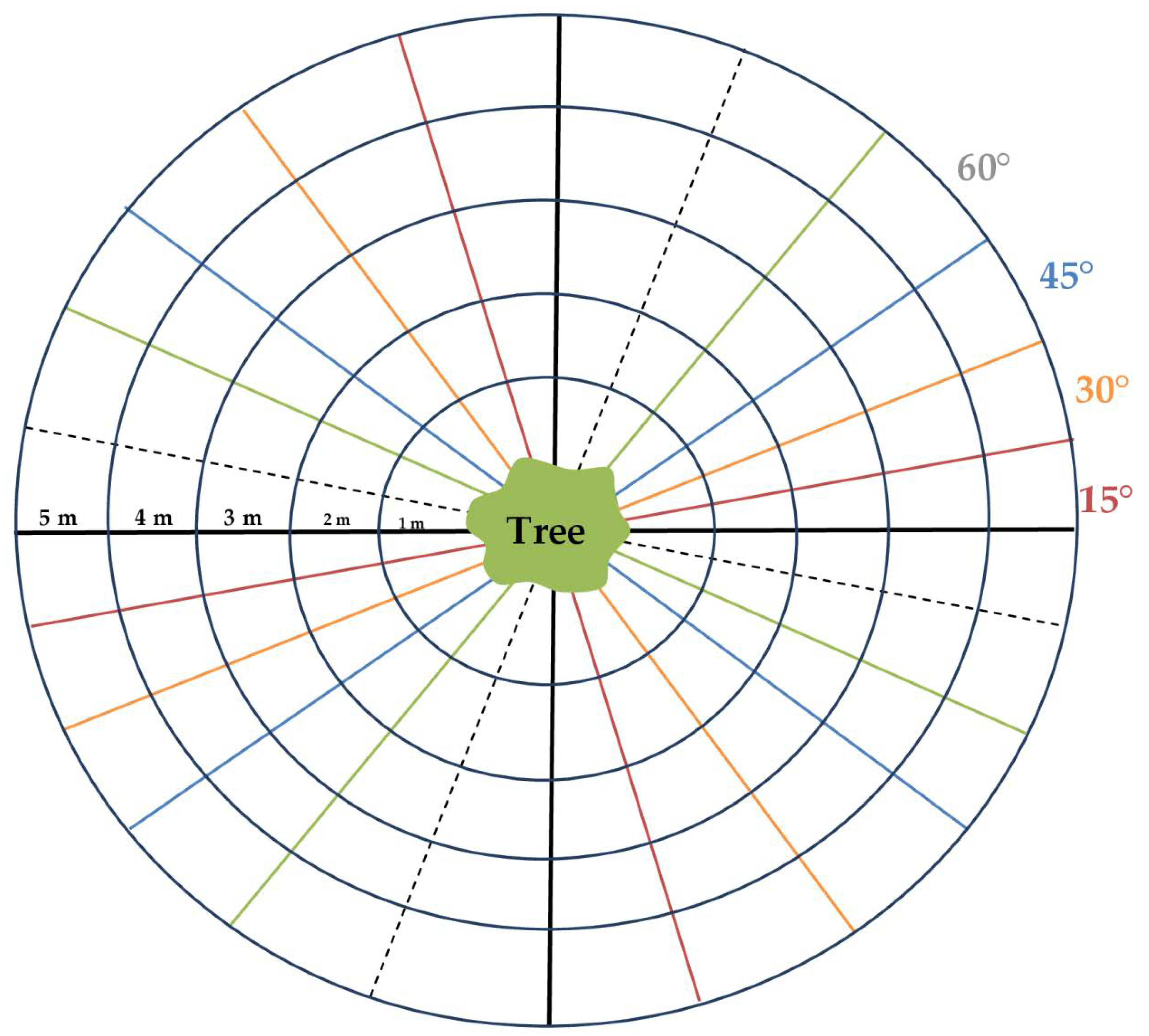
2.3. Image Data Acquisition

Five concentric circles each of radius 1, 2, 3, 4 and 5 m were materialized on the ground around each tree, using the stem as their centre. The circles were then divided into 15° angular sectors to specify 120 potential photographic positions (photopoints), as shown in Figure 2. Thus, photopoints consisted of a combination of five tree-to-camera distances (1, 2, 3, 4 and 5 m) with four regular camera-to-camera positions based on 15°, 30°, 45° and 60° angular shifts. Image acquisition began on the innermost circle and proceeded anticlockwise with an operator capturing photos at 15° intervals all around the tree. Similar circular passes were completed based on 30°, 45° and 60° camera–camera positions, thereby amounting to four image acquisition scenarios at 1 m from the tree. The procedure was repeated 2, 3, 4 and 5 m away from the tree. Thus, for a given tree, 20 photographic datasets, corresponding to each of the 20 image acquisition scenarios, were generated. At each photopoint, highly overlapping photographs (at least 50% vertical overlap between two consecutive photos) were acquired from the base to the treetop. Following these image acquisition schemas, the number of photos would be directly proportional to both shooting distance and angle around a tree. Thus, at 1 m, for example, because of a reduced field of view, more photos would be required to cover the entire stem, using the wide overlap upon which SfM-MVS algorithms rely. Conversely, less photos would be needed farther from the tree. This also applies to shooting angles around a tree, as acquisition schemes based on small angles (e.g., 15°) would yield more photos than those with wider angles, regardless of shooting distance.
A Canon 77 D digital camera equipped with a Canon EF 50 mm f/1.8 STM lens was used throughout image acquisition. This camera is small and lightweight, with a 22.3 × 14.9 mm sensor and a 7.6 cm fully articulated LCD touch screen, which proved useful when shooting overhead on the ground. The camera was held in portrait orientation to ensure maximum coverage of the stem. The operator endeavored to capture vertically overlapping images in parallel to the tree from the base up before moving to the next photopoint. Although our focus was on the main stem, photos were also acquired from a ladder positioned on the designated photopoints. This was done to ensure that the upper portions of the largest tree (height > 12 m) and their crowns were captured for 3-D modeling. Images were saved in JPEG format at the highest resolution (6000 × 4000 pixels). Other important camera settings were ISO: 100 and aperture priority mode (f/3.2).

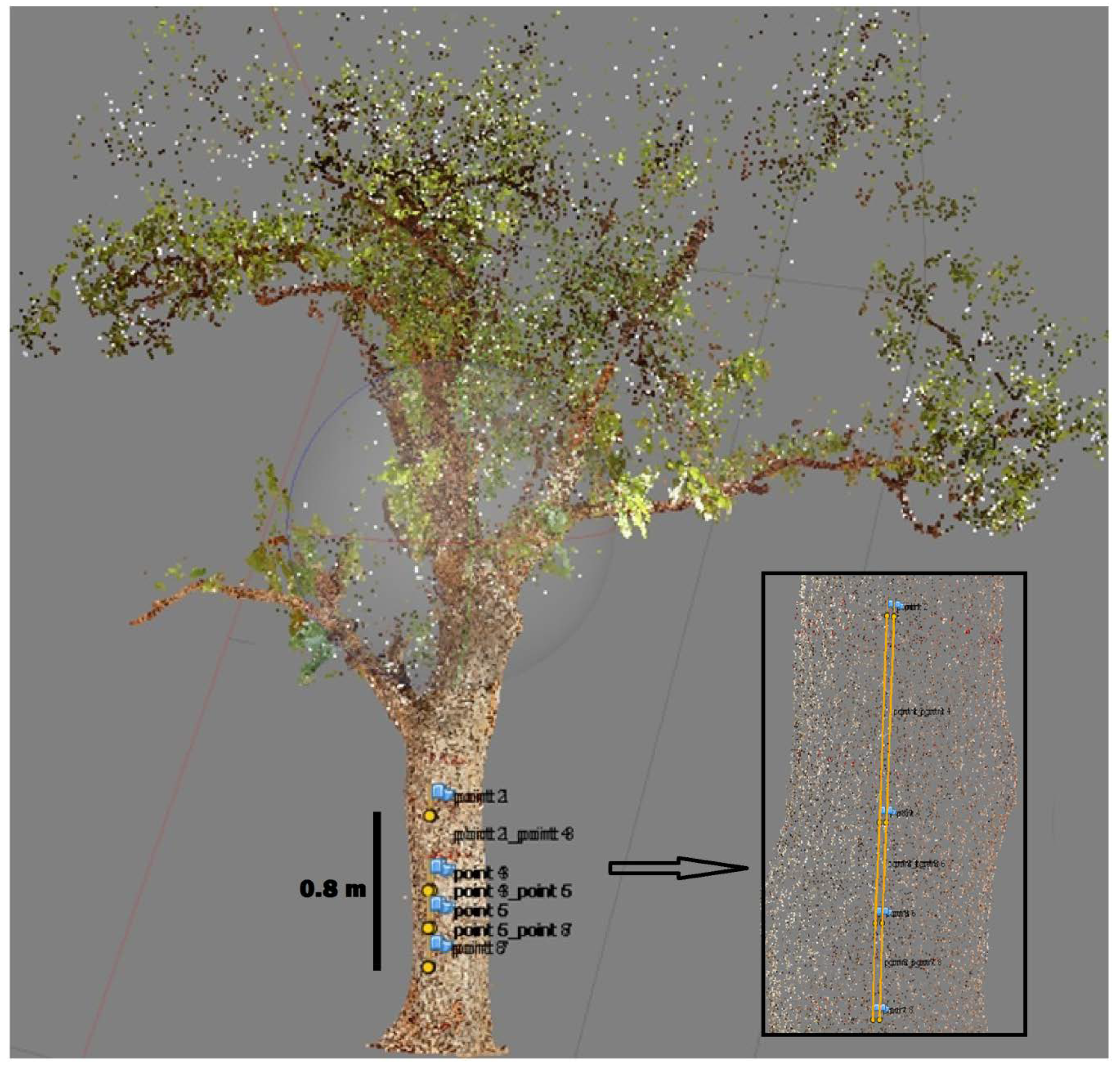
2.4. Image Processing and Metric Estimation

Images were processed using Agisoft PhotoScan Professional version 1, now known as Agisoft Metashape (Agisoft LCC, Saint Petersburg, Russia). PhotoScan uses Structure from Motion (SfM) to simultaneously calculate camera parameters and orientations for each overlapping image pair, and a sparse point cloud that represents matched features in a photographic dataset. This software then applies multi-view stereo algorithms to the sparse point cloud to build a dense point cloud, which can be converted into a textured tridimensional model. Photos from each acquisition scenario were imported into the software environment. The next step was image alignment, which is controlled by four settings, depending on the quality of the resulting sparse point. These settings are (1) “Accuracy”, (2) “Pair pre-selection”, (3) “Key points limit” and (4) “Tie points limit”. We set the highest accuracy to obtain the best estimates of camera positions. Because the camera was not calibrated, the “Generic” image pair pre-selection mode was used to match common features across image pairs. Default settings were used for the number of key points and tie points (40,000 and 1000 respectively). The resulting sparse point cloud model was optimized by carefully removing outliers as recommended. The most important Metashape parameters at the second step are dense point cloud “Quality” and “Depth filtering”. These were set to “high” and the recommended “Aggressive” depth filtering, respectively. Although more steps are available after densification of point cloud to refine 3-D models in Metashape [20], all our tree models were clear enough for metrics estimation and required no further processing. Finally, the coordinate system of the scene was set in order to produce scaled models. This was done using the guided marker placement approach, in which the software automatically calculates marker projections on the rest of the photos (where markers are visible). Eight markers were placed both horizontally and vertically on the markings of a ruler which was vertically pinned to the stem prior to image acquisition (Figure 3). All marker projections were manually refined to minimize scaling uncertainties. Scaled models were saved in a plain text file containing the XYZ coordinates of each point of the dense point cloud.
The coordinate file was analyzed using an open-source GIS application (Quantum GIS version 2.18). All XY points were filtered based on different heights (i.e., by selecting all points in the cloud at the previously defined heights, such as Z = 0.1 m, at the base or Z = 1.3 m, at breast height.) and digitized into a polygon shapefile layer. The resulting polygons represent the cross-section of the stem at the desired heights. Two types of polygons were created, with the first taking into account the shortest distance between two consecutive points, in a way to closely reconstruct the stem cross-sectional profile (Figure 4a). The second polygon type was a simulation of tape-derived circumference measurements for stems with irregular cross-sections. This was created by connecting the closest outermost pair of points with a straight line (Figure 4b). Cross-sectional areas were obtained in QGIS for both polygon types and their corresponding stem circumferences (C1 and C2 respectively) were computed for each height. The main stem of the modeled trees was divided into segments following the heights defined during field measurements with red paint, and the volume was estimated by Smalian’s formula [19]. Similar to field estimates, point cloud-based bole volume was obtained by summing the volume of all stem segments, successively. Two types of volumes (V1 and V2) were calculated in relation to circumference type (C1 and C2, respectively).

2.5. Data Analysis

Because full 3-D models could not be reconstructed from all image acquisition scenarios, we assessed the effect of shooting distance (d), angular shift (α) and tree species identity (s) on 3-D model reconstruction using a logistic regression, as follows
Y i = B ( π i )   and   g ( π i ) = b 0 + b 1 α i + b 2 d i + b 3 s i
where Yi is a binomial variable ( B ( π i ) ); πi the probability of 3-D model reconstruction; αi, di and si variables in image acquisition scenario for a given tree, i, and b0, b1, b2 and b3 regression coefficients.
In cases where full models were rendered, the effect of d, α and s was assessed on the proportion of useful images for each acquisition scenario using a beta regression. The proportion of useful images in a given imaging scenario (Pi) was defined as
P i = 100 ×   N i n i n i
where Ni is the total number of images acquired on the field and ni the number of correctly aligned images (i.e., those for which adequate texture information was available to reconstruct camera position).
Finally, the accuracy of SfM-MVS for breast height circumference and bole volume estimation was assessed in relation to manual field estimates using mean absolute percent error (MAPE) as follows
M A P E = 100 × [ 1 n i = 1 n | P S f M ( i ) P M ( i ) P M ( i ) | ]
where PSfMi and PMi are image-derived and manually estimated metrics for the ith tree and ni the number of trees sampled, respectively. MAPEs were computed based on C1, V1, and C2, and V2, and examined in an analysis of variance with the three factors (α, d and s). All means were separated using the Waller-Duncan test.

3. Results

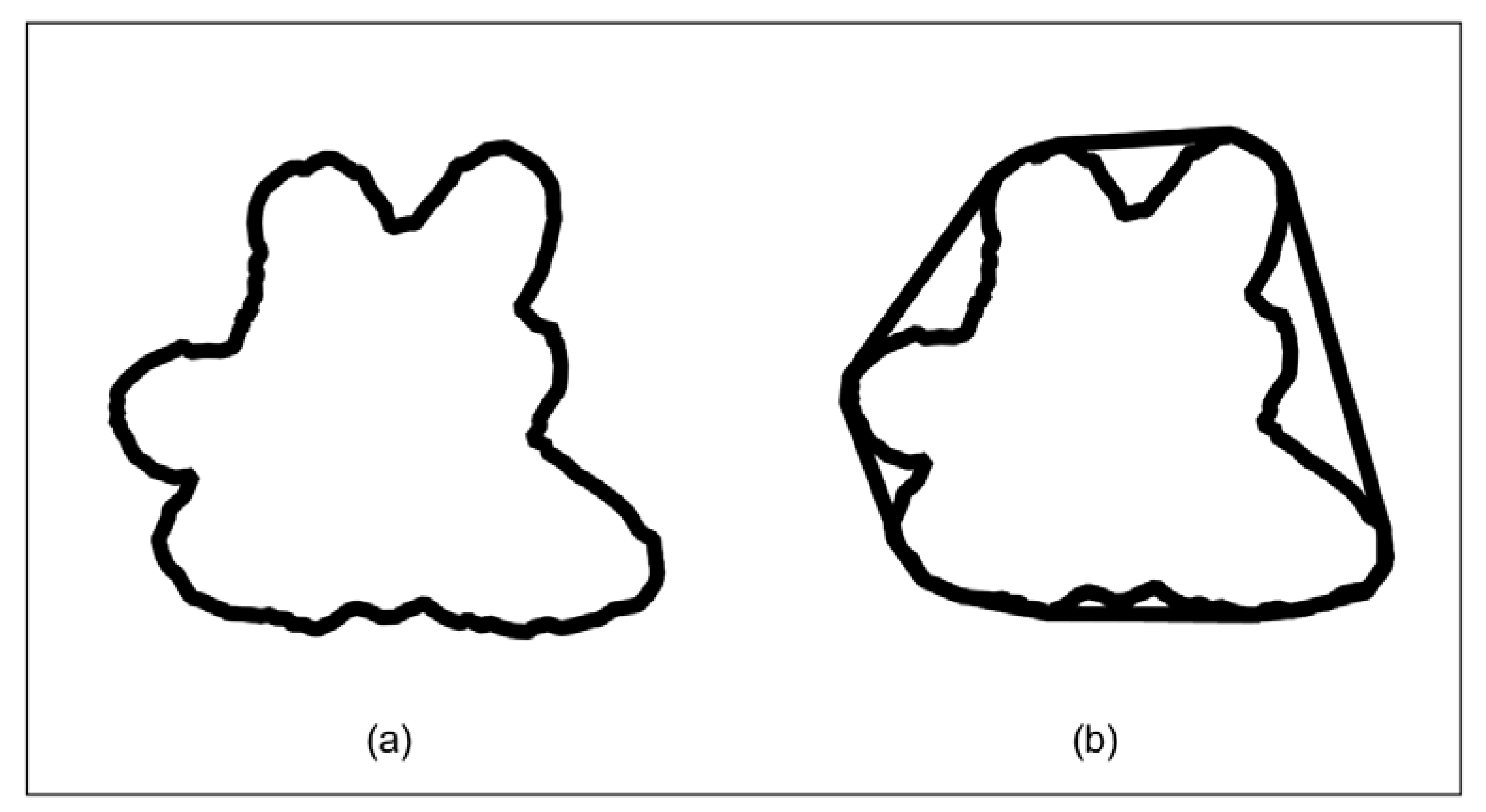
3.1. Individual Tree Model Reconstruction

The result of logistic regression results showed significant differences in 3-D model reconstruction for angular shifts and species identity, with a significant interaction between these two variables (Table 2). In contrast, shooting distance had no significant effect on 3-D model reconstruction. Regardless of species identity, the probability of reconstruction was higher at 15° and 30° (more than 75% and 50%, respectively) as opposed to 45° and 60°, where 3-D rendering failed except for S. birrea (Figure 5A). Data in Figure 5B confirm that shooting distance was not a determining factor in image acquisition for all species.
The results of beta regression showed that the success of model reconstruction differed across angular shifts and species. There were significant differences in the proportion of correctly aligned images, which decreased linearly with increasing angles (Figure 6). The highest proportion of correctly aligned images was obtained at 15° and 30° (Figure 6A). B. costatum and S. birrea had the highest proportion of correctly aligned images (Figure 6B). Species with the lowest 3-D reconstruction probability were S. birrea, followed by T. laxiflora and A. leiocarpa, regardless of shooting distance, whereas, at 30°, S. birrea, A. leiocarpa and V. paradoxa had high proportions of aligned images (Figure 6C). Image alignment failed at wider acquisition angles (45° and 60°), except for S. birrea, which had more than half its images correctly aligned.

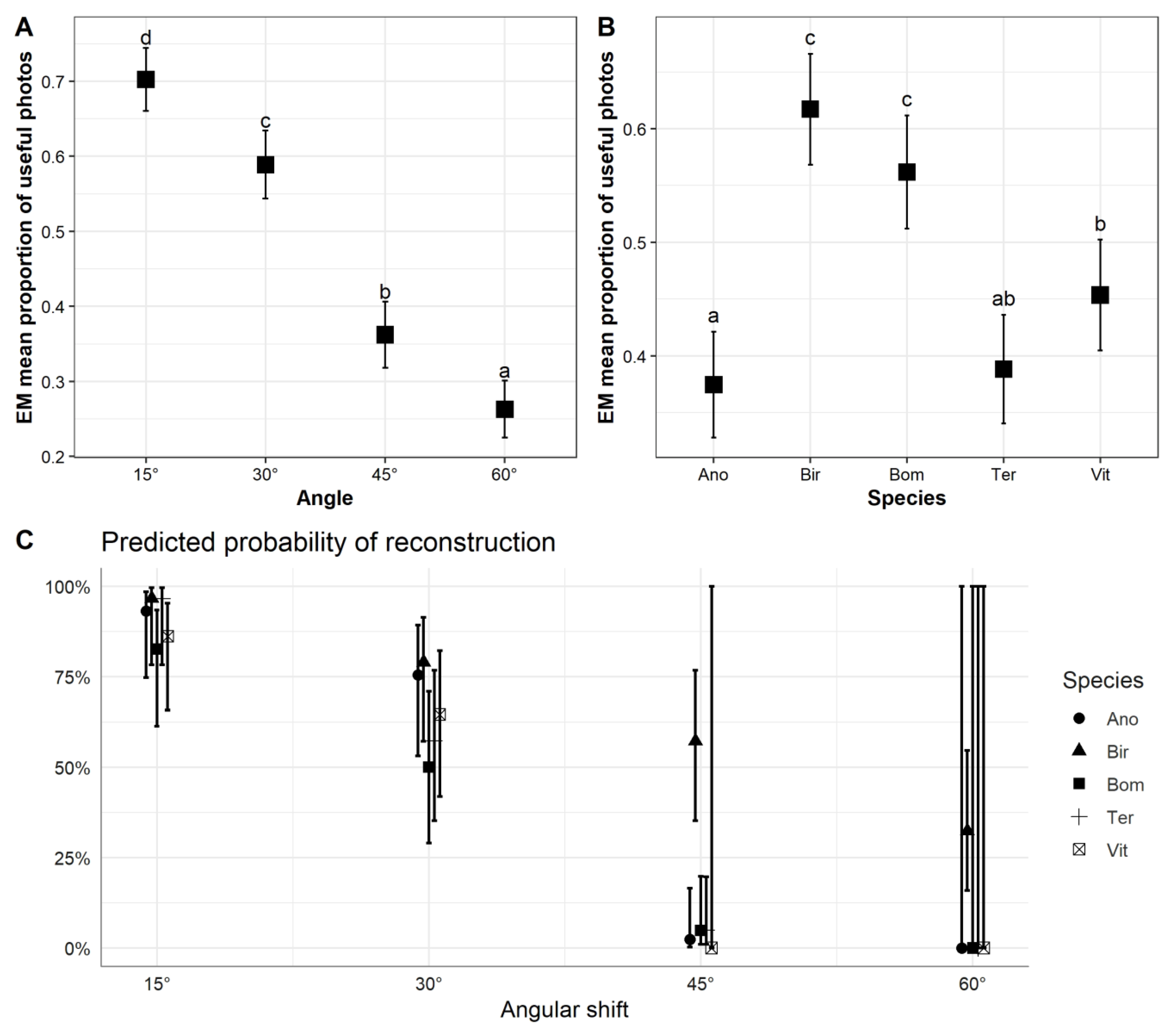
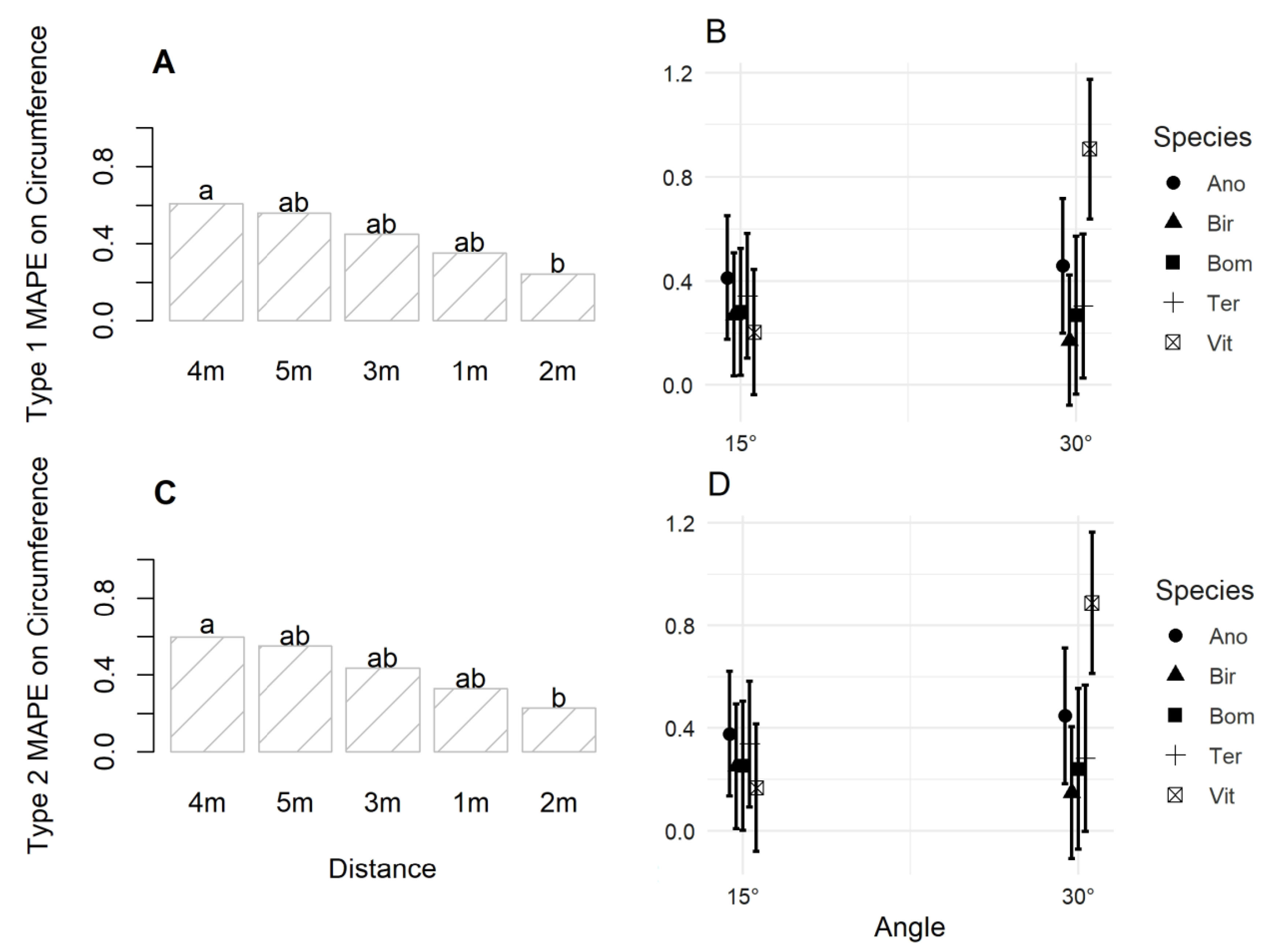
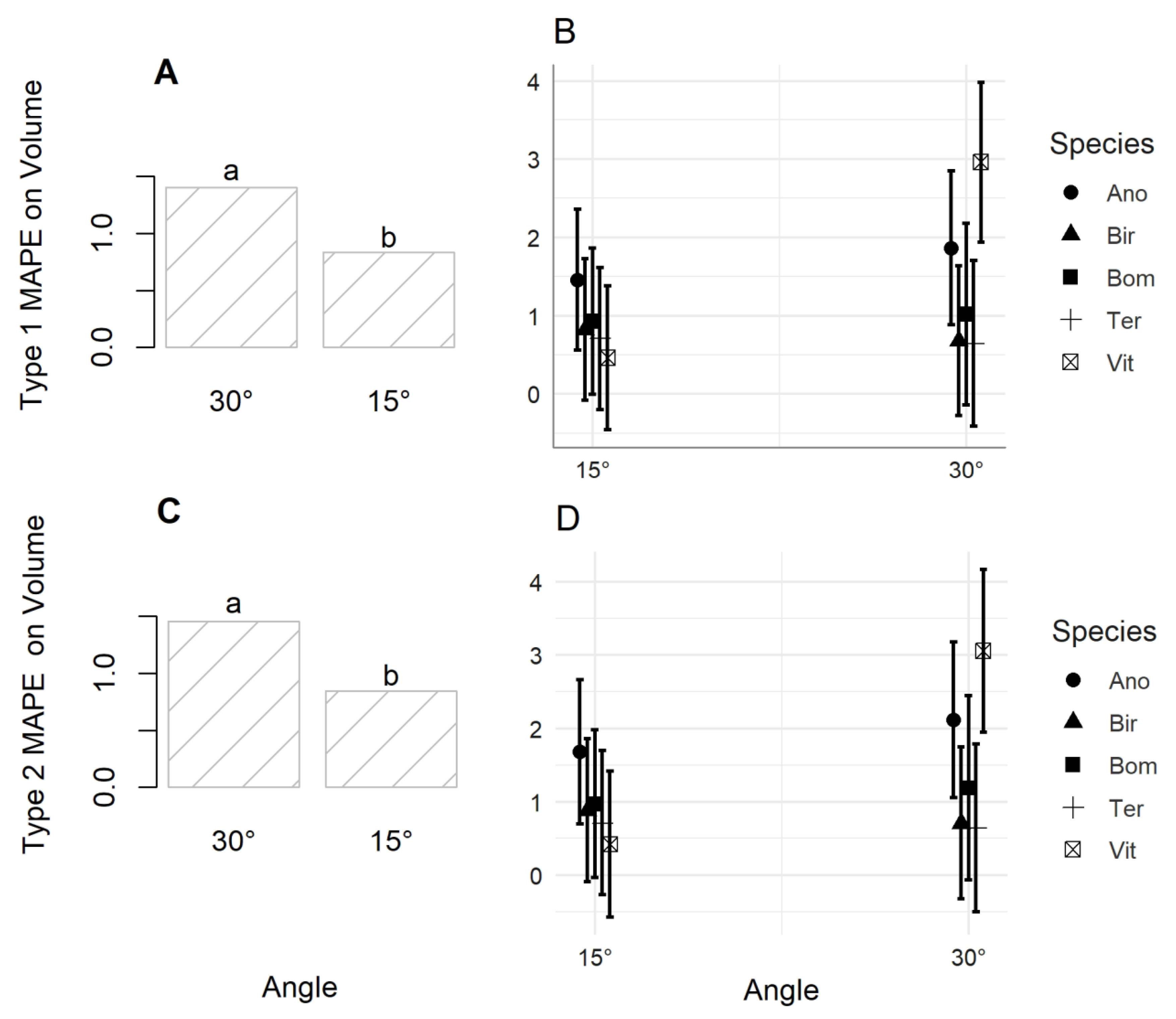
3.2. Accuracy of Image Acquisition Scenarios

Mean absolute percent error on circumference at 1.3 m varied significantly across image acquisition scenarios, with values ranging from 1.6% ± 0.4% (d = 2 m, α = 15°) to 20.8% ± 23.7% (d = 4 m, α = 60°) (Table 3). All images taken 1 m from the tree produced the lowest MAPEs regardless of α. MAPE was about fourfold greater for all acquisition scenarios with d ≥ 2 m and α ≥ 45°. Greater angular shifts (α ≥ 45°) produced less accurate MAPE estimates.
Results are reported for 15° and 30° as imaging schemes based on wider angles (45° and 60°) failed to yield useful 3-D models. Shooting distance had a statistically significant effect on MAPE based on C1, which was highest at 4 m and lowest at 2 m (Figure 7A,C). However, MAPE was not significantly different at 1, 3 and 5 m (depicted by “ab” on corresponding bars). Although angular shift was not significant, MAPE at 15° and 30° varied widely (≈0.4% to 0.9%, respectively) for V. paradoxa as opposed to the other species (Figure 7B,D). Anogeissus leiocarpa had the highest MAPE on breast height circumference at 15°. The lowest errors were recorded on S. birrea and B. costatum at 30°.
Mean absolute percent error computed from tree volume was also dependent on image acquisition scenario and ranged from 2.0% ± 0.6% (d = 1 m, α = 30°) to 36.5% ± 48.7% (d = 4 m, α = 60°) (Table 4). Generally, MAPE increased with both distance and angular shift.
Both angular shift and its interaction with species identity had a significant effect on MAPE based on type 1 volume (V1) (Table 5). As with circumferences, error values computed using V1 and V2 were significantly lower for 15° compared to 30° (Figure 8A,C). Mean absolute percent error on bole volume was lowest in V. paradoxa and highest in A. leiocarpa at 15° (Figure 8B,D). However, shooting with 30° displacements yielded lower errors in T. laxiflora and S. birrea. Vitellaria paradoxa presented the highest error at this angle (Figure 8B,D).
The significant effect of angular displacement and its interaction with species identity obtained with MAPEV1 was mirrored in MAPEV2 (Table 5). However, MAPEV2 differed significantly across species and was lowest for 15° (Figure 8C). Specific MAPEV2 values were 0.603 (T. laxiflora), 0.695 (S. birrea), 0.926 (B. costatum), 1.495 (V. paradoxa) and 1.782 (A. leiocarpa). In line with MAPEV2, the widest variation in MAPEV2 with α was recorded in V. paradoxa and A. leiocarpa (Figure 8D).

4. Discussion

4.1. Individual Tree Model Reconstruction by SFM-MVS

Optimal camera settings, position and orientation vis-à-vis an imaging subject are required to ensure minimum uncertainties in photogrammetric measurements. This study showed that image acquisition scenario for SfM-MVS photogrammetry influences the quality of the 3-D model reconstruction of standing trees. The most useful tree models were obtained using 15° to 30° intervals between consecutive camera positions on a circular path around trees. This is expected due to the inherently higher overlap at these camera positions. Image acquisition scenarios with wider angles (>45°) between two consecutive shooting positions do not guarantee the high photographic overlap on which SfM-MVS algorithms rely [21]. It was also noted that shooting distance had no effect on the success of 3-D model reconstruction. This is mirrored in some previous studies [3,12], where shooting distance was often not defined.
We demonstrated that the success of 3-D model reconstruction and subsequent metric estimation is tree species-dependent. This is in line with the results of Morkoš et al. [6], who showed that root mean square error on stem circumference estimated by SfM-MVS significantly differed across four species, with lower values in Abies alba (0.36%) compared to Fagus sylvatica (0.95%). The five trees investigated in the present study are representatives of four families, namely, Combretaceae (A. leiocarpa and T. laxiflora), Bombacaceae (B. costatum), Anacardiaceae (S. birrea) and Sapotaceae (V. paradoxa). The variation in model quality in relation to species identity may be due to differences in tree physiognomy. During data collection, B. costatum and S. birrea were totally devoid of foliage as opposed to the remaining tree species. The dense canopy and wide-spreading branches of V. paradoxa may explain its low probability of 3-D reconstruction. Although most of the sampled trees here were of moderate heights (6–10 m) and this posed no problem for SfM-MVS reconstruction, our study indicates that tridimensional modeling of individual trees using terrestrial photogrammetry is not recommended for higher trees. We may not have been able to render full 3-D models of trees exceeding 12 m without using a ladder to capture their upper portions. The work of Fang and Strimbu [15] on loblolly pines (approximate height = 24 m) confirms this. In their study, SfM-MVS diameter data could not be obtained on the upper half of tree stems. However, with technological advances, it is expected that terrestrial image acquisition would be supplemented by the use of small, low-cost and low-flying unmanned vehicles, as demonstrated by Gatziolis et al. [1].

4.2. Accuracy of Image Capture Scenarios for Individual Tree Metric Estimation

Results showed that mean absolute percentage error computed between manual and image-derived estimates of stem circumference, as well as volume, varied according to the image acquisition scenario. Accurate tree metrics were obtained with angular shifts below 30° and at shooting distances between 1 to 2 m around a tree, which correspond to arc lengths of 0.26 to 1.04 m, respectively. Values within this range have been reported in previous studies [6,16]. So far, the effects of image capture scenarios on tree metric estimation has only been assessed at the plot level [2,13]. Although direct comparisons between plot-based and tree-level image collection methods may not be feasible, one relevant point can be noted from these studies. The application of the mobile acquisition method (in which shooting is done continuously [13]) to individual tree metric estimation may not produce useful data, as opposed to the stop-and-go mode. Thus, the spatial configuration of camera positions around an imaging subject remains one of the major determinants of success in SfM-MVS photogrammetry.
Tree metric estimation from the most useful image capture scenarios yielded an accuracy level similar to those found in past studies. Bias values between SfM-MVS and manually measured breast height diameters of 9.6% and 3.7% were reported by Miller et al. [4] and Morgenroth and Gomez [3], respectively. Similarly, the difference in stem volume estimations between these two methods was in the order of 12%, as in Miller et al. [4], although lower values have been reported [22].
The major limitation of this method lies in the time constraint associated with the use of a single camera for image acquisition. However, Mulverhill [17] showed that individual tree metrics could be accurately estimated in just four minutes of field work using a simple imaging method based on two cameras. Furthermore, considerably shorter times (<2 minutes) have been reported in plot-based forest inventories using more than two cameras [11]. These studies underscore the potential advantages of SfM-MVS in forestry, especially in terms of cost and time efficiency. Although lightning conditions may also constitute another drawback to the application of SfM-MVS, especially in dense forests [11], the use of an external source of light such as built-in flash could be helpful [10]. However, this would be the issue of least concern in physiognomically simple ecosystems such as savannas and other sparsely forested habitats.

5. Conclusions

This study aimed at prescribing an optimal image acquisition scenario for a satisfactory 3-D model reconstruction and subsequent metric extraction using savanna trees. Shooting distances ranging from 1 to 5 m away from a tree subject were considered in conjunction with four angular shifts. Our assessment of the 3-D model reconstruction potential of spatially different image acquisition scenarios using five tree species underscored the importance of maintaining a very high degree of overlap between consecutive image pairs. Thus, the accuracy of individual tree metrics estimated from photogrammetric point clouds is tied to proximity to imaging subject. The use of multiple cameras may reduce the time of photogrammetric data collection.

Author Contributions

Methodology, Investigation, Formal Analysis, Funding acquisition, Writing—original draft, H.A.A.; Supervision, Formal Analysis, Writing—review & editing, Validation, G.A.; Methodology, Investigation, Writing—original draft, review and editing, M.C.O.; Data Curation, Investigation A.B.A. and M.G.; Conceptualization, Resources, P.L.; Project administration, Supervision, Formal Analysis, Validation, Writing—review & editing, N.H.F. All authors have read and agreed to the published version of the manuscript.

Funding

This research was funded by the International Foundation for Science (Grant No: I-1-D-6066-1).

Conflicts of Interest

The authors declare no conflict of interest.

References

  1. Gatziolis, D.; Lienard, J.F.; Vogs, A.; Strigul, N.S. 3D Tree Dimensionality Assessment Using Photogrammetry and Small Unmanned Aerial Vehicles. PLoS ONE 2015, 10, e0137765. [Google Scholar] [CrossRef] [PubMed] [Green Version]
  2. Liang, X.; Wang, Y.; Jaakkola, A.; Kukko, A.; Kaartinen, H.; Hyyppä, J.; Honkavaara, E.; Liu, J. Forest Data Collection Using Terrestrial Image-Based Point Clouds From a Handheld Camera Compared to Terrestrial and Personal Laser Scanning. IEEE Trans. Geosci. Remote. Sens. 2015, 53, 5117–5131. [Google Scholar] [CrossRef]
  3. Morgenroth, J.; Gomez, C. Assessment of tree structure using a 3D image analysis technique—A proof of concept. Urban For. Urban Green. 2014, 13, 198–203. [Google Scholar] [CrossRef]
  4. Miller, J.; Morgenroth, J.; Gomez, C. 3D modelling of individual trees using a handheld camera: Accuracy of height, diameter and volume estimates. Urban For. Urban Green. 2015, 14, 932–940. [Google Scholar] [CrossRef]
  5. Surový, P.; Yoshimoto, A.; Panagiotidis, D. Accuracy of Reconstruction of the Tree Stem Surface Using Terrestrial Close-Range Photogrammetry. Remote Sens. 2016, 8, 123. [Google Scholar] [CrossRef] [Green Version]
  6. Mokroš, M.; Výbošt’ok, J.; Tomaštík, J.; Grznárová, A.; Valent, P.; Slavík, M.; Merganĭc, J. High Precision Individual Tree Diameter and Perimeter Estimation from Close-Range Photogrammetry. Forests 2018, 9, 696. [Google Scholar] [CrossRef] [Green Version]
  7. Westoby, M.J.; Brasington, J.; Glasser, N.F.; Hambrey, M.J.; Reynolds, J.M. ‘Structure-from-Motion’ photogrammetry: A low-cost, effective tool for geoscience applications. Geomorphology 2012, 179, 300–314. [Google Scholar] [CrossRef] [Green Version]
  8. Huang, H.; Zhang, H.; Chen, C.; Tang, L. Three-dimensional digitization of the arid land plant Haloxylon ammodendron using a consumer-grade camera. Ecol. Evol. 2018, 8, 5891–5899. [Google Scholar] [CrossRef] [PubMed]
  9. Piermattei, L.; Karel, W.; Wang, D.; Wieser, M.; Mokroš, M.; Surový, P.; Koreň, M.; Tomaštík, J.; Pfeifer, N.; Hollaus, H. Terrestrial Structure from Motion Photogrammetry for Deriving Forest Inventory Data. Remote Sens. 2019, 11, 950. [Google Scholar] [CrossRef] [Green Version]
  10. Koeser, A.K.; Roberts, J.; Miesbauer, J.W.; Lopes, A.B.; Kling, G.J.; Lo, M.; Morgenroth, J. Testing the Accuracy of Imaging Software for Measuring Tree Root Volumes. Urban For. Urban Green. 2016, 18, 95–99. [Google Scholar] [CrossRef]
  11. Forsman, M.; Börlin, N.; Holmgren, J. Estimation of Tree Stem Attribute Using Terrestrial Photogrammetry with a Camera Rig. Forests 2016, 7, 61. [Google Scholar] [CrossRef]
  12. Liu, J.; Feng, Z.; Yang, L.; Mannan, A.; Khan, T.U.; Zhao, Z.; Cheng, Z. Extraction of sample plot parameters from 3D point cloud reconstruction based on combined RTK and CCD continuous photography. Remote Sens. 2018, 10, 1299. [Google Scholar] [CrossRef] [Green Version]
  13. Mokroš, M.; Liang, X.; Surový, P.; Valent, P.; Černăva, J.; Chudý, F.; Tunák, D.; Salon, S.; Merganič, J. Evaluation of Close-Range Photogrammetry Image Collection Methods for Estimating Tree Diameters. ISPRS Int. J. Geoinf. 2018, 7, 93. [Google Scholar] [CrossRef] [Green Version]
  14. Iglhaut, K.; Cabo, C.; Puliti, S.; Piermatteit, L.; O’Connor, J.; Rosette, J. Structure from Motion Photogrammetry in Forestry: A Review. Curr. For. Rep. 2019, 5, 155–168. [Google Scholar] [CrossRef] [Green Version]
  15. Fang, R.; Strimbu, B.M. Stem Measurement and Taper Modeling Using Photogrammetric Point Clouds. Remote Sens. 2017, 9, 716. [Google Scholar] [CrossRef] [Green Version]
  16. Roberts, J.W.; Koeser, A.K.; Abd-Elrahman, A.H.; Hansen, G.; Landryd, S.M.; Wilkinson, E. Terrestrial photogrammetric stem mensuration for street trees. Urban For. Urban Green. 2018, 35, 66–71. [Google Scholar] [CrossRef]
  17. Mulverhill, C.; Coops, N.C.; Tompalski, P.; Bater, C.W.; Dick, A.R. The utility of terrestrial photogrammetry for assessment of tree volume and taper in boreal mixedwood forests. Ann. For. Sci. 2019, 76, 83. [Google Scholar] [CrossRef] [Green Version]
  18. Zakari, S.; Tente, B.A.H.; Yabi, I.; Toko, I.I. Evolution hydroclimatique, perceptions et adaptation des agroéleveurs dans l’extrême nord du Bénin (Afrique de l’Ouest). In Actes Du 28ème Colloque De L’AIC; Liège: Wallonie, Belgique, 2015; pp. 399–405. [Google Scholar]
  19. Picard, N.; Saint-André, L.; Henry, M. Manual for Building Tree Volumes and Biomass Allometric Equations: From Field Measurement to Prediction; Food and Agriculture Organization of the United Nations (FAO): Rome, Italy, 2012; pp. 1–215. [Google Scholar]
  20. Agisoft, L.L.C. Agisoft Metashape User Manual: Professional Edition, Version 1.5; Agisoft LLC: St. Petersburg, Russia, 2019; Available online: https://www.agisoft.com/pdf/metashape-pro_1_5_en.pdf (accessed on 31 December 2019).
  21. Lowe, D.G. Distinctive image features from scale-invariant keypoints. Int. J. Comput. Vis. 2004, 60, 91–110. [Google Scholar] [CrossRef]
  22. Hopkinson, C.; Chasmer, L.; Young-Pow, C.; Treitz, P. Assessing forest metrics with a ground-based scanning lidar. Can. J. For. Res. 2004, 34, 573–583. [Google Scholar] [CrossRef] [Green Version]
Figure 1. Map of study area.
Forests 11 00121 g001
Figure 2. Illustration of image acquisition scenarios.
Forests 11 00121 g002
Figure 3. Scaled 3-D model of V. paradoxa. Image acquisition was on a circular path, 1 m from the stem, based on 15° angular shifts.
Forests 11 00121 g003
Figure 4. A stem cross-section reconstructed from a sparse point cloud. Type 1 (C1) and Type 2 (C2) circumferences are convex hulls based on the shortest distance between any two vertices (a) and a straight line between the closest outermost vertices (b).
Forests 11 00121 g004
Figure 5. Tri-dimensional model quality in relation to tree species identity and angular shift (A), and distance (B). Ano: Anogeissus leiocarpa; Bom: Bombax costatum; Bir: Sclerocarya birrea; Ter: Terminalia laxiflora; Vit: Vitellaria paradoxa.
Forests 11 00121 g005
Figure 6. Proportion of useful images in relation to angular shift (A) and species (B). Predicted probability of the reconstruction of species-specific 3-D models is also shown in relation to angular shift (C). Ano: Anogeissus leiocarpa; Bom: Bombax costatum; Bir: Sclerocarya birrea; Ter: Terminalia laxiflora; Vit: Vitellaria paradoxa. Means with different letters (a, b, c and d) are statistically different (Waller-Duncan test, p < 0.05).
Forests 11 00121 g006
Figure 7. MAPE of breast height circumference in relation to distance (A,C) and species (B,D). Ano: Anogeissus leiocarpa; Bom: Bombax costatum; Bir: Sclerocarya birrea; Ter: Terminalia laxiflora; Vit: Vitellaria paradoxa. Histogram bars with different letters (a and b) differ significantly (Waller-Duncan test, p < 0.05).
Forests 11 00121 g007
Figure 8. MAPE of stem volume in relation to angular shift (A,C) and species (B,D). Ano: Anogeissus leiocarpa; Bom: Bombax costatum; Bir: Sclerocarya birrea; Ter: Terminalia laxiflora; Vit: Vitellaria paradoxa. Histogram bars with different letters (a and b) are significantly different (Waller-Duncan test, p < 0.05).
Forests 11 00121 g008
Table 1. Descriptive statistics of the sampled trees.
MetricSpeciesMeanS.DCV %MinimumMaximum
A. leiocarpa135.4078.7058.1446.50275.00
B. costatum127.3060.3047.3644.00198.00
CBH (cm)S. birrea130.5072.8055.7951.00239.00
T. laxiflora131.1053.3040.6361.50202.00
V. paradoxa125.6053.9042.9343.70195.00
Total130.1060.4046.6243.70274.90
A. leiocarpa2.280.9441.361.323.97
B. costatum3.600.9726.842.344.65
HStem (m)S. birrea2.490.7931.601.483.75
T. laxiflora2.560.9336.231.334.02
V. paradoxa2.860.3412.012.503.35
Total2.780.9132.691.324.80
A. leiocarpa10.002.6226.25.8913.78
B. costatum10.103.7036.74.9114.64
HT (m)S. birrea10.143.2331.876.2013.00
T. laxiflora9.542.0221.146.3011.50
V. paradoxa9.342.0622.116.4612.60
Total9.822.6326.734.9114.64
CBH: Breast height circumference, HStem: bole height, HT: Total height, S.D: Standard deviation, CV: Coefficient of variation (n = 6).
Table 2. Results of logistic regression of camera-tree distance (d), angular displacement (α) and species identity (s) on 3-D model reconstruction.
DfDevianceResid. DfPr(>Chi)
NULL 599
d47.025950.135
α3348.80592<0.001 ***
s474.98588<0.001 ***
α × s1230.635760.002 **
d × α1210.905640.538
d × s1617.955480.327
d × α × s4816.39500>0.999
** Pr < 0.01; *** p < 0.001.
Table 3. Mean absolute percent error (MAPE) of stem circumference at breast height for all combinations of shooting distances and angular shifts.
α
15°30°45°60°Mean ± SEM
d (m)11.6 ± 0.5 aA1.8 ± 0.6 aA7.7 ± 17.8 bA1.7 ± 13.3 aA2.1 ± 0.9 A
21.6 ± 0.4 aA2.2 ± 0.7 aA8.1 ± 11.5 bA7.4 ± 51.4 bB2.5 ± 0.8 A
310.4 ± 2.9 aB10.6 ± 4.0 aB10.2 ± 2.6 aB7.5 ± 4.7 aB10.3 ± 1.9 B
414.5 ± 4.3 aC15.5 ± 5.1 aC18.2 ± 13.1 aC20.8 ± 23.7 aC15.7 ± 2.9 C
515.4 ± 3.1 aC15.5 ± 3.8 aC13.2 ± 12.2 aC15.9 ± 0.0 aC15.3 ± 2.1 C
Mean ± SEM8.3 ± 1.5 a9.2 ± 1.9 a11.2 ± 3.1 a11.6 ± 7.0 a9.0 ± 1.1
Data are means ± standard error. Values in each row followed by different lowercase superscripts (a and b) are significantly different, as are those with different uppercase superscripts (A, B and C) in each column (Waller-Duncan test, p < 0.05).
Table 4. MAPE of stem volume estimation for combinations of shooting distances and angular shifts.
α
15°30°45°60°Mean ± SE
d (m)13.0 ± 0.7 aA2.0 ± 0.6 aA22.6 ± 45.2 bA3.7 ± 16.6 aA4.2 ± 2.4 A
22.5 ± 0.6 aA2.6 ± 0.7 aA7.9 ± 14.4 aA6.6 ± 46.3 aA3.1 ± 0.8 A
312.6 ± 3.7 aB15.8 ± 5.9 aB14.3 ± 6.6 aA11.2 ± 4.1 aA13.9 ± 2.8 B
422.4 ± 7.0 aC18.8 ± 5.0 aBC22.1 ± 35.8 aA36.5 ± 48.7 aA22.0 ± 4.6 C
524.6 ± 5.0 aC25.0 ± 6.20 aC26.2 ± 12.6 aA33.7 ± 0.0 aA25.0 ± 3.40 C
Mean ± SEM12.2 ± 2.3 a12.9 ± 2.6 a17.5 ± 6.9 a19.5 ± 13.9 a13.3 ± 1.70
Data are means ± standard error. Values followed by different lowercase superscripts (a and b) in each row differ significantly as do those with different uppercase superscripts (A, B and C) in each column (Waller-Duncan test, p < 0.05).
Table 5. ANOVA summary results of MAPE of stem circumference and volume.
Significance (ANOVA Summary)
dαsd × α Interactiond × s Interactionα × s Interactiond × α × s Interaction
MAPEC10.010 *0.1080.0870.6660.9740.007 **0.774
MAPEC20.011 *0.1030.1130.6430.9760.007 **0.755
MAPEV10.7560.039 *0.0730.1910.9130.023 *0.913
MAPEV20.6520.037 *0.049 *0.2020.8680.030 *0.912
p values on 3-way ANOVA of shooting distance, angular shift and species identity on effects. Data are the means ± standard error and the t-test results are shown (* p < 0.05 and ** p < 0.01).

