Time-Lag Effect Between Sap Flow and Environmental Factors of Larix principis-rupprechtii Mayr
by
 ,
,
Liu Hong
1, 
Jianbin Guo
1,*,
Zebin Liu
2,
Yanhui Wang
2,
Jing Ma
1,2,
Xiao Wang
2 and
Ziyou Zhang
1,2 1
College of Soil and Water Conservation, Beijing Forestry University, 35 East Qinghua Road, Beijing 100083, China
2
Key Laboratory of Forestry Ecology and Environment of the State Forestry Administration of China, Research Institute of Forest Ecology, Environment and Protection, Chinese Academy of Forestry, Beijing 100091, China
*
Author to whom correspondence should be addressed.
Forests 2019, 10(11), 971; https://doi.org/10.3390/f10110971
Submission received: 25 August 2019
/
Revised: 22 October 2019
/
Accepted: 30 October 2019
/
Published: 3 November 2019
(This article belongs to the Special Issue Water Cycling and Drought Responses of Forest Ecosystems)
Abstract
:A time lag between sap flux density (Js) and meteorological factors has been widely reported, but the controlling factors of the time lag are poorly understood. To interpret the time lag phenomenon systematically, thermal dissipation probes were placed into each of eight trees to measure the Js of Larix principis-rupprechtii Mayr. in the Liupan Mountains in Northwest China. Meteorological factors, including vapor pressure deficit (VPD), solar radiation (Rs) and air temperature (Ta), were synchronously measured with Js, and the dislocation contrast method was used to analyze the time lag between Js and the meteorological factors. The analysis indicated the following for the whole experimental period. (1) The time lag between Js and VPD (TLV) and the time lag between Js and Rs (TLR) both exhibited different patterns under different weather conditions, and Js could precede Rs on dry days. (2) Both TLV and TLR varied with the day of the year (DOY) throughout the experimental period; namely, both exhibited a decreasing tendency in September. (3) Reference crop evapotranspiration (ETref) had a greater influence on the time lag than the other meteorological factors and directly controlled the length and direction of TLV and TLR; relative extractable water (REW) modified the relationship between ETref and time lag. (4) The regression analysis results showed differences between the time lags and the environmental factors (ETref and REW) within different ranges of REW. Namely, TLR was better determined by ETref and REW when REW < 0.38, while TLV was better correlated with ETref and REW in the absence of soil water limitations (REW > 0.38). This project provided an important opportunity to advance the understanding of the interaction between plant transpiration and meteorological factors in a changing climate.
1. Introduction
Plant transpiration accounts for 61% (±15% s.d.) of evapotranspiration and returns approximately 39% ± 10% of incident precipitation (P) to the atmosphere, creating a dominant force in the global cycle [1,2]. Transpiration regulation by plants is a key process that underlies vegetation drought responses and land evaporative fluxes under global change scenarios [3]. However, our knowledge of plant water strategies as well as the interaction between forests and climate in temperate forests remains unclear [4], especially given increases in drought occurrence [5,6,7], which have put tremendous pressures on forests and caused extensive death among various species [8,9].
The hysteresis loop has long been a topic of great interest in a wide range of fields, including hydrology, ecology and plant physiology [10,11,12,13]. Time lag is another form of hysteresis that is defined as the time difference between peak values of Js and meteorological variables [14], the length and direction of a time lag can, in turn, reflect the magnitude of hysteresis [12], and the time lag between sap flux density (Js) and environmental factors is often identified as a self-protection mechanism of plants to avoid dehydration [15]. Therefore, with increasingly frequent extreme weather events, investigating time lags is a continuous concern regarding plant and water relationships.
Time lags, which affect hourly and daily patterns of sap flow, exist widely among different tree species. Accordingly, studies have determined that ignoring time lags can instantaneously result in errors of up to 30% when estimating canopy transpiration [16]. Additionally, it has been observed that the peak sap flux density consistently lags behind solar radiation (Rs) and precedes the vapor pressure deficit (VPD) [17,18]. Moreover, significant seasonal variations have also been reported in previous studies [19,20], and the results vary in different regions. For example, a study in eucalyptus open forests indicated that the degree of hysteresis between Js and VPD was larger in the winter than in the summer [21], whereas both Zeppel et al. [22] and Zhang et al. [11] drew contrasting conclusions. Zeppel et al. [22] noted that the different results (larger hysteresis in the winter than in the summer) may have been due to the low soil moisture during winter in the study region, and Zhang et al. [11] attributed this phenomenon to increased resistance between soil and roots; thus, soil water cannot be immediately transported to stems (or leaves), and as a result, the gap between water demand and supply is larger during this period than at other times. Nonetheless, researchers have not studied this seasonality in much detail. Hence, it is hoped that this research will contribute to a deeper understanding of phenological variations in time lags.
The factors influencing time lags have been explored in several studies, and the paradox in the response of time lag to soil moisture has drawn much attention over time. Wullschleger et al. [23] found that hysteresis was much more evident in wet soil, whereas Tuzet et al. [24] found that the area of the hysteretic loop increased as soil moisture declined. Moreover, Zhang et al. [11] reported that the time lag was poorly correlated with soil moisture. The mechanisms that underpin how soil moisture affects time lags are not fully understood and need to be studied further. However, to date, few studies have investigated the relationship between reference crop evapotranspiration (ETref) and time lags although this variable represents the evaporative demand of the atmosphere [25] and therefore could be a key factor affecting the balance between water supply and demand. In addition, previous studies of hysteresis have only focused on the time lag between Js and VPD (known as TLV) [12,21,22,23,24], and few studies have investigated the time lag between Js and Rs (known as TLR) in any systematic way. The experimental work presented here provides one of the first investigations into the theoretical explanation of how ETref and relative extractable water (REW) affect TLR.
Larix principis-rupprechtii Mayr. is one of the major species used for afforestation in Northwest China [26]; this species shows moderate cold resistance, grows in many types of soils and has become one of the most important plantation in the Liupan Mountains in Ningxia, China [27,28]. In recent years, research on sap flow in Larix principis-rupprechtii has mostly focused on variation characteristics and its variability at different temporal and spatial scales [29]. Guan et al. [30] mentioned in a study of Larix principis-rupprechtii that the start time of sap flux density lagged 1 h behind the sunrise time; however, there has been no quantitative research on the time lag impact or on the major causes of the time lag, and both of these factors limit an in-depth understanding and precise estimate of diurnal canopy transpiration variations in Larix principis-rupprechtii.
The purpose of this paper was to interpret the interaction of evaporative demand and soil moisture supply in determining the length and direction of both TLV and TLR. Hence, to achieve this goal, we used thermal dissipation probes [31] to measure the sap flux density of Larix principis-rupprechtii in the Xiangshui River Basin in the Liupan Mountains from 25th May to 30th September 2017 and hypothesized the following: (1) The time lag would exhibit different patterns under three different weather conditions, namely, sunny days, overcast days and rainy days. (2) The time lag would exhibit significant seasonal variation in the study period that could be ascribed to the effects of variations in environmental factors, namely, solar radiation, vapor pressure deficit, reference crop evapotranspiration and relative extractable water. (3) Finally, reference crop evapotranspiration would be the key factor that directly controls the length and direction of the time lag, while relative extractable water would modify the relationship between reference crop evapotranspiration and time lag.
2. Materials and Methods
2.1. Study Site and Plant Materials
This study was conducted at Xiangshuihe, a small watershed (106°12′–106°16′ E, 35°27′–35°33′ N) in the nature reserve of the Liupan Mountains in Northwest China, which belongs to the warm temperate and semihumid zone. The mean annual air temperature and precipitation in this area are 5.8 °C and 618 mm, respectively, and most of the annual precipitation occurs from June to September. The annual sunshine hours range from 2100–2400 h (1374 h during the study period), and the number of frost-free days ranges from 90–130 days. The vegetation is dominated by natural secondary forests of Pinus armandii Franch., Quercus liaotungensis Koidz., Betula platyphylla Sukaczev. and Betula albosinensis Burk., with an area of 25.3 km2. The plantation area is composed of 90% Larix principis-rupprechtii, with an area of 10.4 km2.
The sample plot was a 36-year-old plantation (in 2017) with Larix principis-rupprechtii growing on the Southeast hillslope that had an area of 30 × 30 m2, a stand density of 948 stem/ha, an elevation of 2524 m above sea level, and a slope gradient of 36°. The mean diameter at breast height (DBH) and tree height at the site were 20.21 cm and 17.07 m, respectively. The crown diameter was 3.1 m. The soil type at the site was lixisols with a sandy loam texture. This plantation had several shrubs, including Rosa omeiensis Rolfe., Prunus salicina Lindl., Fargesia nitida (Mitford) Keng f., and Cotoneaster acutifolius Turcz. Furthermore, Fragaria orientalis Lozinsk. and Carex spp. were the dominant species in the herbaceous layer. The coverage of understory vegetation (shrubs and herbs) was low, with a shrub layer coverage of 15% and herb layer coverage of 40%, due to the high canopy density of 0.74. Sap flux density and environmental measurements used in this study were collected between May and September 2017, and the withered leaves in Larix principis-rupprechtii at this site was observed on 27th September.
2.2. Meteorological Factors and Soil Water Measurements
Meteorological factors, such as solar radiation (Rs, w/m2), air temperature (Ta, °C), relative humidity (RH, %), wind speed (m/s) and wind direction, were measured every 5 minutes with a weather station (Weatherhawk232, Weatherhawk, Logan, UT, USA) that was located in an open field approximately 100 m away from the sample plot to avoid canopy interference and to comply with meteorological factors. The vapor pressure deficit (VPD, kPa) was calculated based on meteorological data as follows:
where is the atmospheric air temperature (°C) and is the relative humidity (%).
The reference crop evapotranspiration (, mm) was calculated using the FAO Penman Monteith equation [25]:
where Δ is the slope of the curve relating saturated vapor pressure to temperature (kPa/°C), is the net radiation (MJ/m2), is the soil heat flux (MJ/m2), is the psychrometric constant (kPa/°C), is the mean air temperature (°C), is the wind speed at 2 m height (m/s), and VPD is the saturation vapor pressure deficit (kPa).
The REW at 0–60 cm depth was continually monitored every 5 minutes using probes (ECH2O-5TE, Decagon Devices, Inc., Pullman, WA, USA) connected to a data logger (model Em50/R, Decagon Devices, Inc., Pullman, WA, USA). These sensors measure the volumetric water content by measuring the dielectric constant of a medium using a 70 MHz capacitance/frequency. The REW can reflect the soil water available for transpiration and was calculated as the ratio of the actual extractable water to the maximum extractable water [15]:
where VSM is the volumetric soil moisture of the 0–60 cm soil layer (%), is the minimum VSM, and is the maximum VSM in the study period.
2.3. Sap Flux Density Measurement
The sap flux density was measured with heat dissipation sensors. The thermal probes (SF-L, Ecomatik, Munich, Germany) consisted of four sensors that were 20 mm in length and 2 mm in diameter: , a heated sensor powered by a constant current of 12 V; , an unheated sensor; and and , reference sensors. These sensors were installed into the outer 20 mm of the xylem at breast height on the North side of the tree trunks. The data were collected with a data logger (Delta-T, Cambridgeshire, England) every 5 minutes. Eight sample trees representing different DBH ranges were selected to continuously monitor the sap flux density (Table 1).
() was computed as follows:
where are the air temperature differences (°C) between and , and , and and , respectively, is the maximum air temperature difference when sap flux density ceases, is the instant air temperature difference, n is the sample size of the sap flux density measurements, () is the sap flux density of the ith sample, and Ai is the sapwood area of the ith sample (cm2).
In this study, the sapwood thickness of most trees in the plot did not exceed 40 mm, and we assumed that Ji was constant across the sapwood profile within a smaller range of changes [32], allowing the whole-tree Ji to be estimated by Ji in the 0–20 mm sapwood depth range.
2.4. Dislocation Movement Method
The dislocation movement method was used to assess the relationship between the time lags in stem sap flow and meteorological factors. The synchronized time series of sap flux density and meteorological data were shifted with a time step of 5 minutes, and the time lag that led to the maximum correlation coefficient was obtained [11,33]. Note that throughout this paper, a positive value of time lag or clockwise loops between Js and environmental factors indicate that the peak in sap flux density occurs earlier in the day than that of environmental factors, while a negative value of time lag or counterclockwise loops between Js and environmental factors indicate that the peak in sap flux density occurs later in the day than that of environmental factors.
2.5. Statistical Analysis
Using data from May to September 2017, an average sap flux density dataset was established, along with the synchronized meteorological factors. To test whether time lag would exhibit different patterns under different weather conditions, we divided time lag into three groups (sunny days, overcast days and rainy days), and analysis of variance (ANOVA) was used to analyze the differences among groups.
We used linear regression analysis to explore the relationship between time lag and the daily mean environmental factors (Rs, VPD, ETref and REW). Additionally, to eliminate confounding effects in Rs and VPD and to test the direct effects of the two individual variables on time lag, Rs-normalized time lags were obtained by using the residuals from the relationship between time lag and Rs, and VPD-normalized time lags was obtained by using the residuals from the relationship between time lag and VPD [34].
To determine the impact of soil water limitation on the time lag, we divided REW into 2 groups (REW < 0.38 and REW > 0.38). REW = 0.38 is the threshold value that induces stomatal closure in this plant, which was obtained by using boundary line analysis between Js and REW (Supplementary Figure S1). ANOVA was used to analyze the difference between the two REW groups. Multiple regression analysis was used to explore the impacts of ETref and REW on TLV and TLR at different REW categories. The standardization of the coefficient was used to determine which of the independent variables have a greater effect on the time lag.
ANOVA was conducted by IBM SPSS 21.0 (IBM Corp., New York, NY, USA). The linear regression analysis and multiple regression analysis were performed using R software (version 3.4.2), standardized coefficient of ETref and REW used the mvstats package in R [35]. All curves were fit with SigmaPlot 12.5 software (Systat Software Inc., San Jose, CA, USA).
3. Results
3.1. Seasonal Variations in Sap Flux Density and Environmental Factors
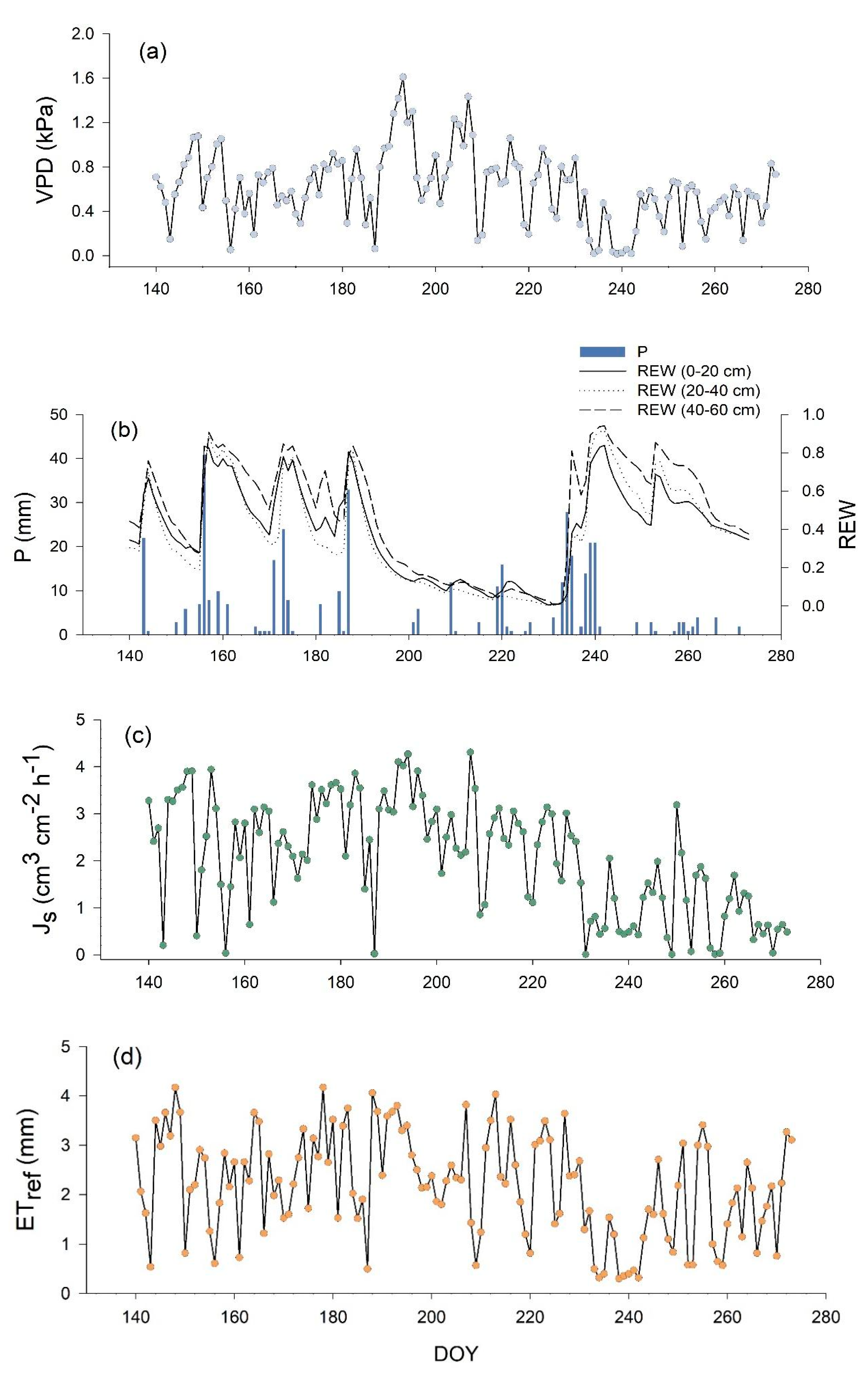
Figure 1 presents the seasonal variations in the mean daily Js and the environmental factors during the experimental period. VPD varied from 0.015–1.61 kPa and reached the maximum value in July and the minimum value in September. The REW at a 0–60 cm soil depth increased significantly during periods when large precipitation (P) amounts occurred. The daily average sap flux density reached the maximum value on the 25th of July (4.36 cm3 cm−2 h−1) and the minimum value on the 18th of September (0.007 cm3 cm−2 h−1). ETref ranged from 0.3–4.17 mm, and its variations were similar to those of Js; both parameters remained at a higher level in spring and summer and decreased in autumn, which indicates a connection between sap flow and evapotranspiration demand.
3.2. Diurnal Variations in Sap Flux Density and Meteorological Factors
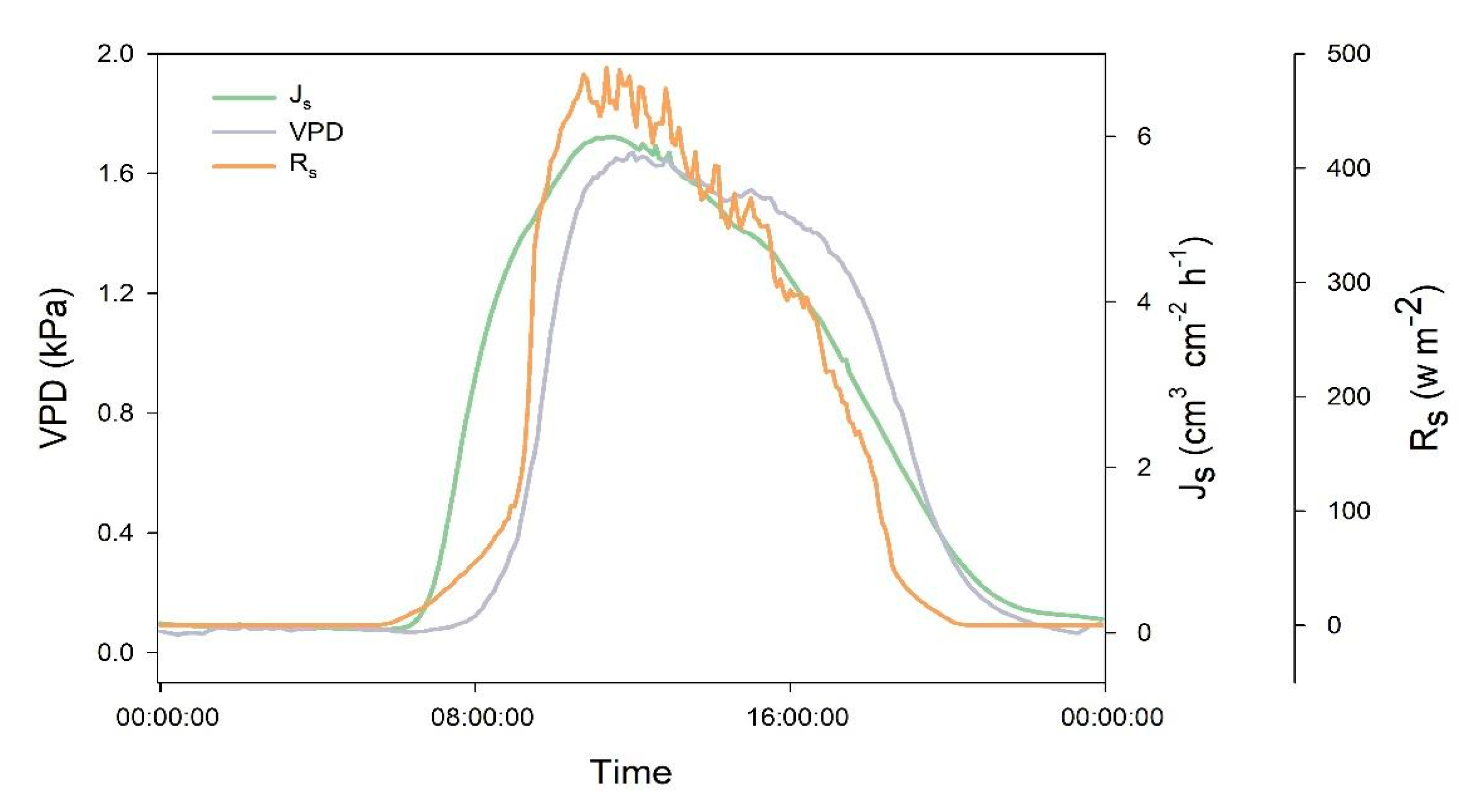
The diurnal variations in the sap flux density and meteorological factors throughout the growing season are shown in Figure 2. Js increased gradually at approximately 6:00, then increased as Rs increased, and peaked at 11:30. The trends in the two values were basically the same. Rs peaked at 11:20, preceding Js by approximately 10 min. VPD lagged 0.5 h behind Js and peaked at 12:00.
3.3. Time Lag Variations under Different Weather Conditions
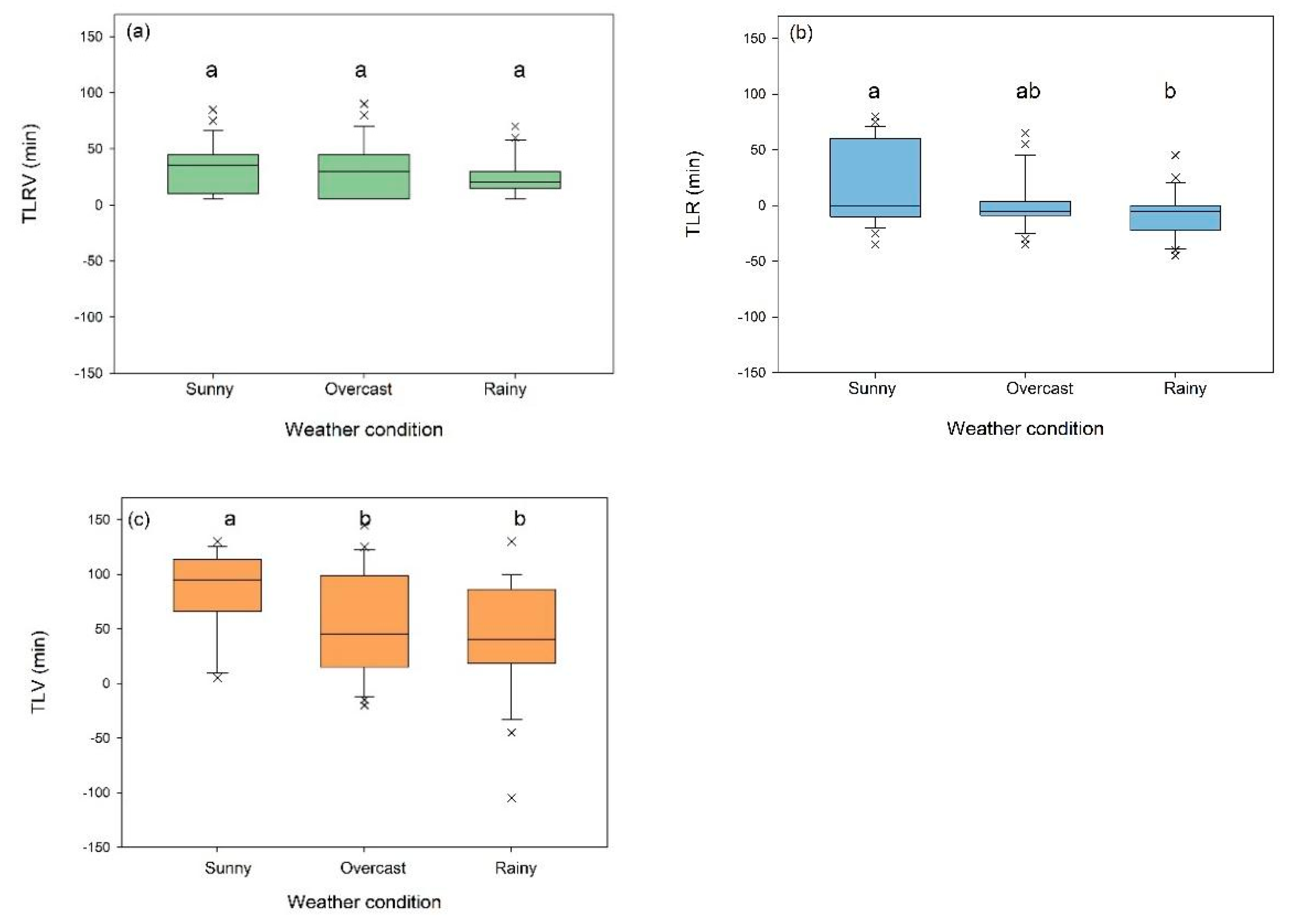
The differences in the time lag under different weather conditions are highlighted in Figure 3. For the time lag between VPD and Rs (TLRV), no significant differences were found among sunny days, overcast days and rainy days, but for TLR, there was a significant difference between sunny days and rainy days, while for TLV, significant differences were found between sunny days and other weather conditions. The median TLR values were similar in the three different weather conditions, but the TLR values in the upper quartiles were considerably higher on sunny days compared to the results obtained in other weather conditions. The median TLV values on sunny days were higher than those in other weather conditions, but there were negative extreme outlier values on overcast and rainy days. TLRV remained positive in all conditions.
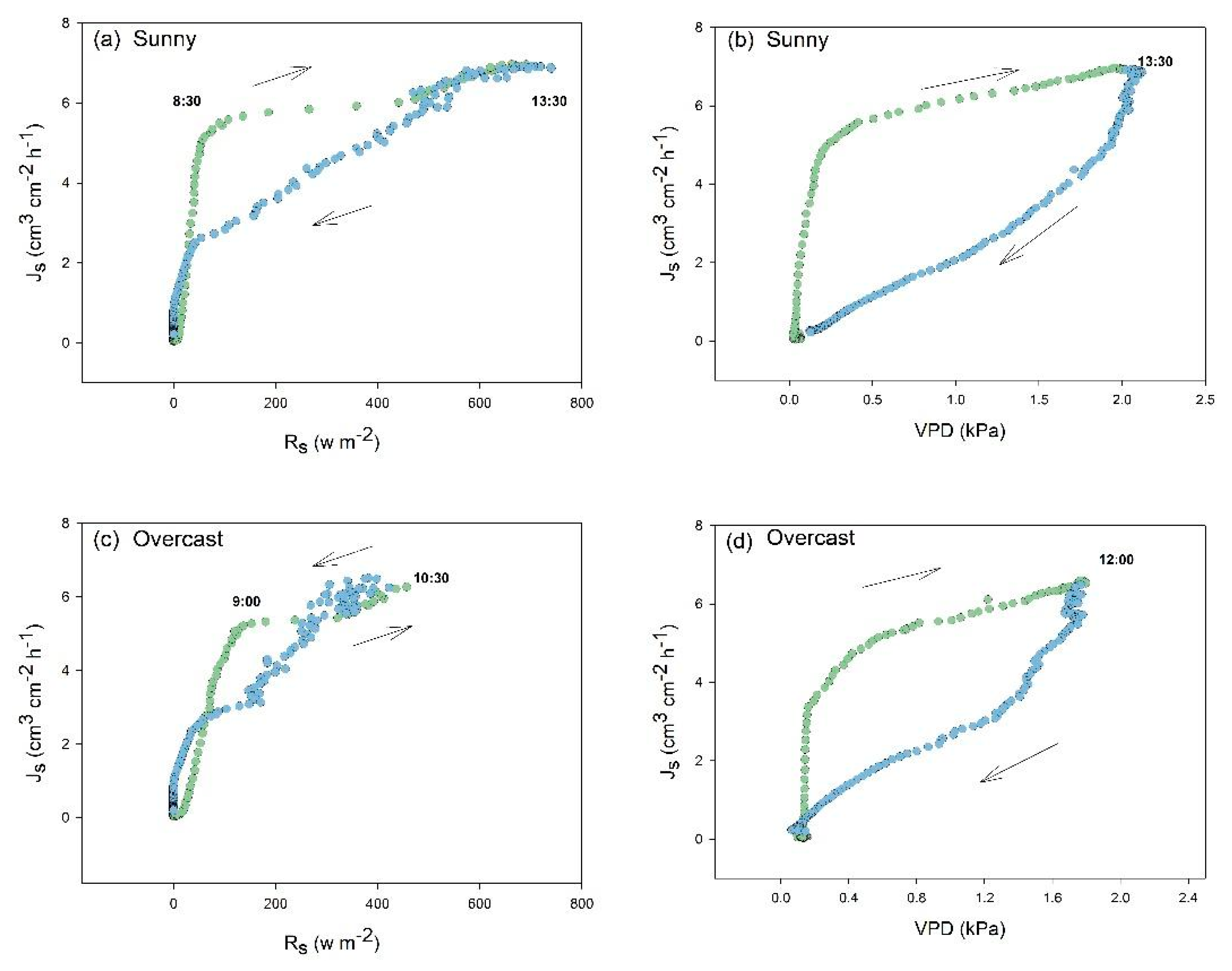
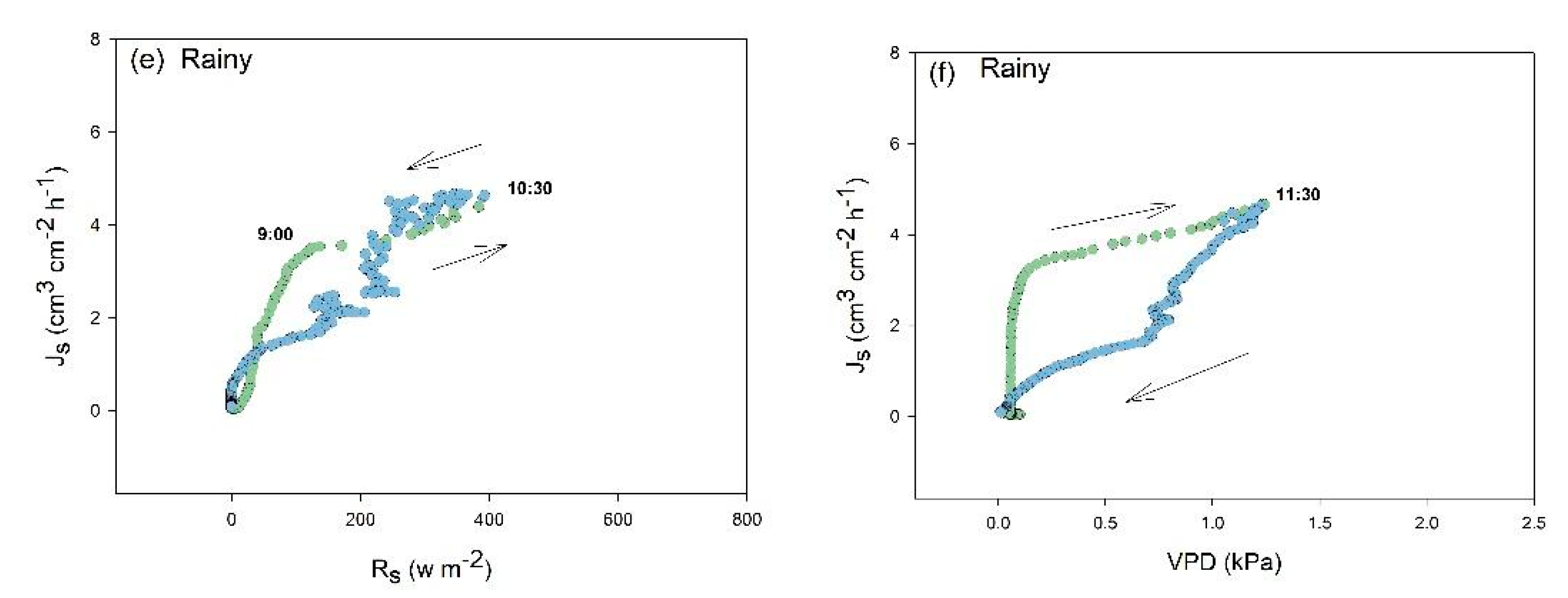
The hysteresis loop similarly exhibited different patterns under different weather conditions (Figure 4): The magnitude of the hysteresis loop between Js and Rs was mostly clockwise on sunny days, while the magnitude of the counterclockwise part was larger during overcast and rainy days. The hysteresis loop between Js and VPD revealed a clockwise pattern, and the magnitude of the hysteresis on sunny days was significantly larger than that on overcast and rainy days.
3.4. Time Lag Fluctuations between Sap Flow and Meteorological Factors during the Growing Season
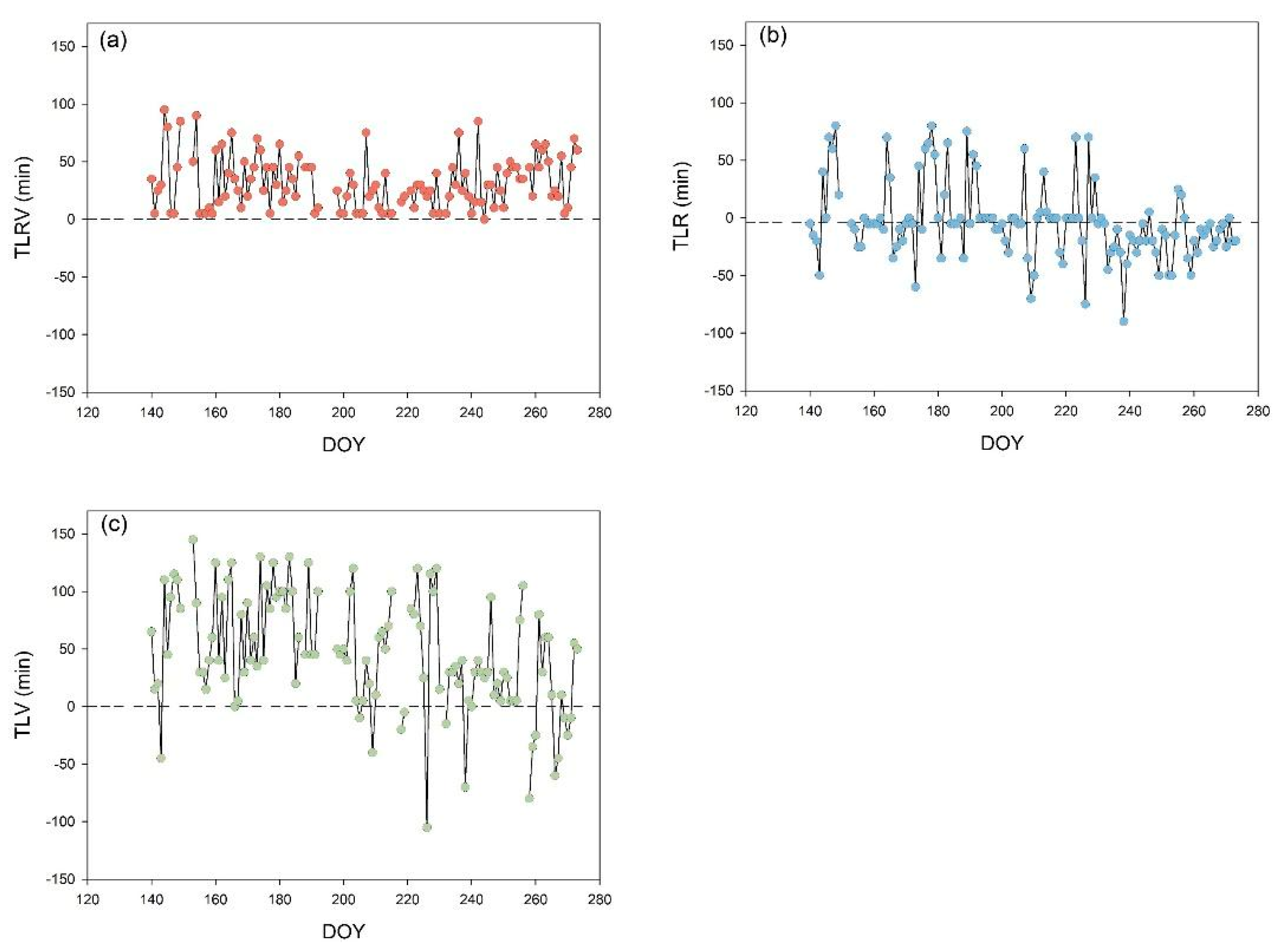
The figure below illustrates that the time lags all exhibited significant fluctuations during the whole growing period (Figure 5). The results showed that TLRV was lower in summer and higher in spring and autumn, whereas both TLR and TLV exhibited a significant decrease in September.
3.5. Time Lag Response to Different Environmental Factors
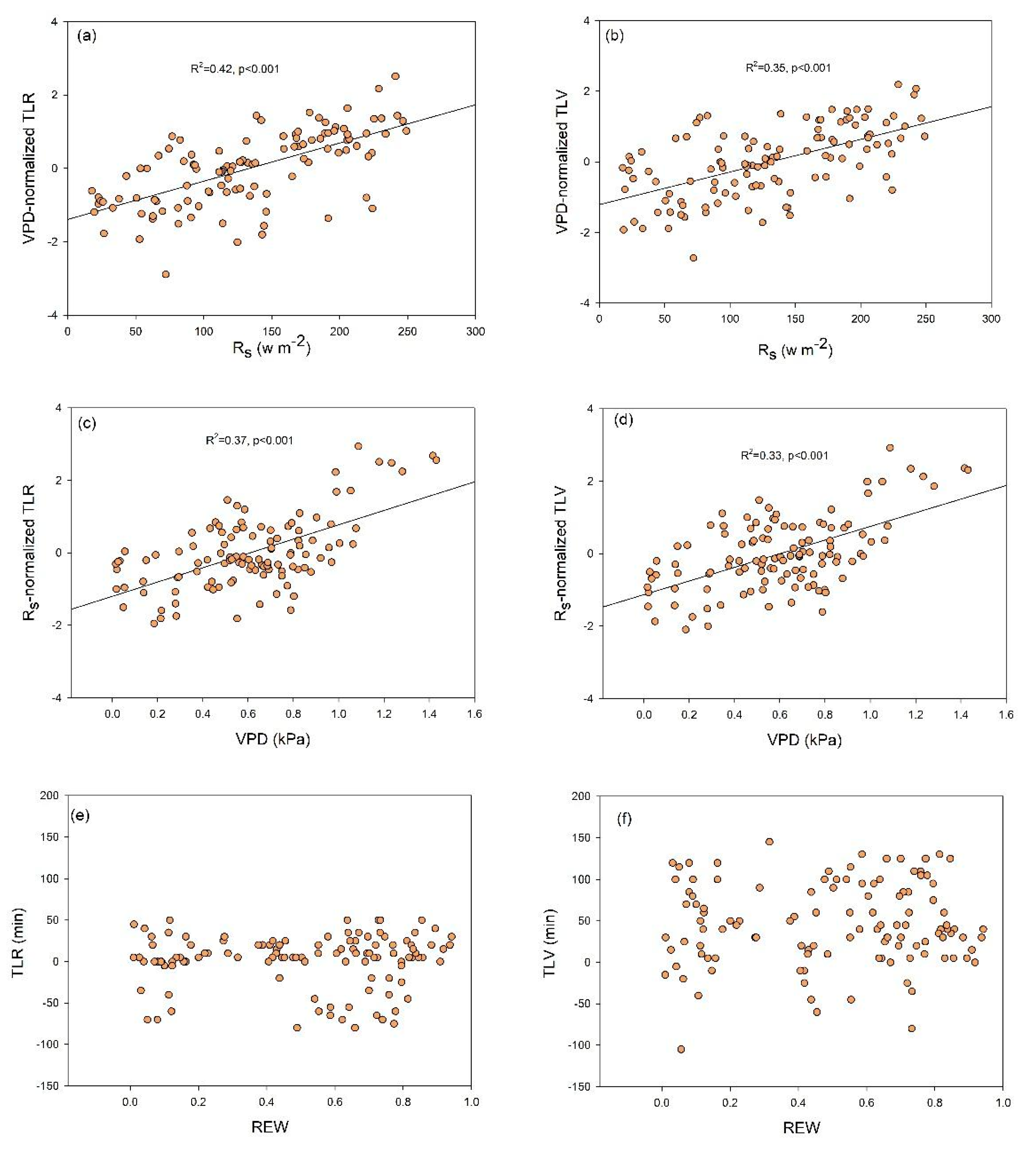
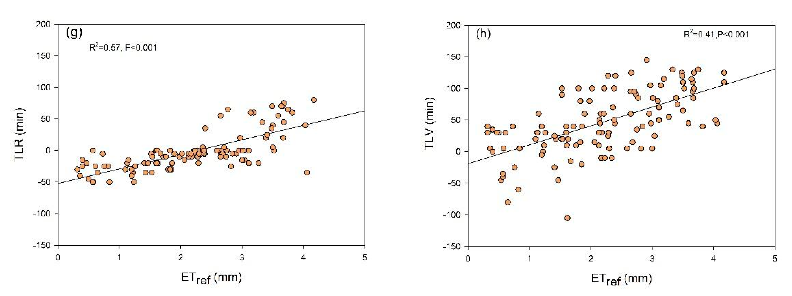
Notably, as shown in Figure 6, Rs and VPD were positively related to normalized time lags with determination coefficients generally being above 0.3. Moreover, a significant positive correlation was found between ETref and the time lag, with determination coefficients of 0.57 for TLR and 0.41 for TLV. However, no significant correlation was found between time lag and REW.
As shown in Table 2, REW showed a rather strong negative connection with TLR when REW < 0.38, with a standardized coefficient of REW of −0.213; however, a weak positive influence on TLR was observed when the water supply was sufficient (REW > 0.38), while ETref showed strong positive correlations with TLR in both REW categories with standardized coefficients generally being above 0.7. Additionally, REW were positively related to TLV and did not affect it differently under the two soil water conditions, and the positive effect of ETref on TLV was more evident in wet soils (REW > 0.38) than in dry soils (REW < 0.38). Moreover, the TLV did not fit well with ETref and REW when REW < 0.38, with a determination coefficient of 0.278.
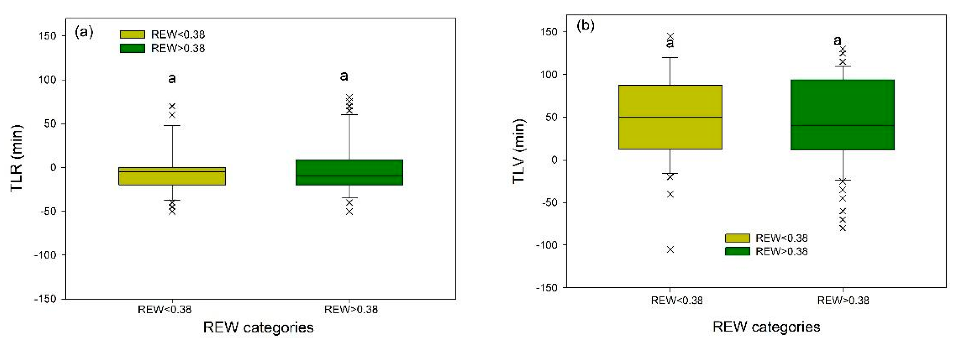
In addition, as shown in Figure 7, in both TLR and TLV, no significant differences were found between the two REW categories except that the median TLR value (−5 min) was slightly higher when REW < 0.38 compared with REW > 0.38 (−10 min); similarly, the median TLV value (50 min) was a bit higher when REW < 0.38 compared with REW > 0.38 (40 min).
4. Discussion
4.1. Seasonal Variation in Time Lag
In reviewing the literature, the phenomenon of Js lagging behind Rs and preceding VPD has been widely reported [20,21,22,23,24,36,37]. However, our results were both similar to and different from previous studies. We investigated the time lag under different weather conditions, and the results suggested that there was a significant difference between sunny days and rainy days for TLR, while for TLV, significant differences were found between sunny days and other weather conditions. The phenomenon of Js lagging behind Rs often occurred on overcast and rainy days; however, one unanticipated finding was that Js could precede Rs on sunny days but lag behind VPD on some rainy days.
Js lagging behind Rs is a rather common phenomenon, since solar radiation peaks at noon, while VPD peaks in the afternoon; consequently, Js would be larger in the afternoon than in the morning at a given Rs, and thus, a counterclockwise loop would be formed [22]. However, on dry days, Js preceding Rs is inevitable, since stomatal conductance becomes light-saturated at very low levels of light early in the morning with limited available water [38], but the plant water storage was not enough to maintain the high transpiration rate at the light-saturated point, therefore, water stress will cause the partial stomatal closure or increasing of plant hydraulic resistance, which in turn decreases the transpiration rate; as a result, a clockwise loop is formed, and a positive value is obtained.
Regarding Js-VPD hysteresis, VPD peaked in the afternoon and increased the stomatal sensitivity. Therefore, stomatal closure in plants can be induced, resulting in reduced water use and leading to clockwise hysteresis between Js and VPD [22]. In other words, any time lag between VPD and Rs could result in a time lag between Js and VPD [12]. Longer hysteresis often occurred with stomatal closure and a high VPD; therefore, the phenomenon that Js precedes VPD can also be seen as a self-protection mechanism to avoid excessive water loss by adjusting the time period between the peaks in Js and VPD [15]. In addition, on overcast and rainy days, Js could lag behind VPD; this phenomenon has also been reported in a humid low-energy headwater catchment in recent research [14]. A possible explanation for this scenario might be the rather weak influence of VPD on Js; on rainy days, stomatal sensitivity has a poor relationship with VPD due to a sufficient water supply and relatively high humidity, and the influence of VPD on the stomata could diminish under this circumstance. Therefore, it can be assumed that when time lags are relatively large, the possibility of plant water stress may be enhanced.
Another important finding was the variation in time lag at different times of the year, which was consistent with previous studies [36,37,39]. In a study of Larix gmelinii (Rupr.) Kuzen., Wang et al. found that there were no significant variations in each season for TLR [36]; however, in a study of Haloxylon ammodendron (C. A. Mey.) Bunge in the Minqin oasis-desert ecotone in 2018, Yao et al. found that TLR was longer in both September and May than in other seasons, while TLV reached its maximum in September [37]. These differences can be explained in part by differences in variation in the environmental factors that determine the imbalance of the water demand and water supply. Moreover, precipitation differences could lead to differences in soil moisture and VPD [11], which are closely related to time lags and contributed to the different results in other studies.
In this paper, the time lag between Rs and Js was shortened in September and was relatively high at the beginning of the growing season, while TLV exhibited a pattern that contrasted with that of the former. These results are likely related to seasonal alterations that caused a decrease in air temperature along with relatively low transpiration rate in the later period of the growing season. These joint forces may have minimized excessive plant water loss as well, leading to a decreasing tendency in both TLV and TLR. In other words, a lower evaporative demand will result in fewer opportunities to cause stomatal closure at noon; thus, a lower TLR value was found in September. For TLV, the time lag in autumn was short compared to those in other seasons, which may be explained by the fact that VPD could have had less of an influence on transpiration when frequent precipitation occurred in September, which resulted in higher moisture levels and a lower TLV at that time.
4.2. Influence of Environmental Factors on Variations in Time Lag
Prior studies have noted the importance of both soil moisture and meteorological demands in controlling time lags [22,40,41]. However, most studies in the field have only focused on the influence of VPD on time lags while neglecting the effects of comprehensive meteorological factors, such as ETref, that directly reflect evapotranspiration demand. Far too little attention has been paid to TLR, although this metric may provide a way to reflect plant water stress through the size of hysteresis as TLV functioned [12]. Hence, in this paper, REW (reflecting the water capacity of shallow root systems that are related to the water uptake process) and ETref (a comprehensive meteorological factor that reflects the evapotranspiration demand in the plant canopies) as well as Rs and VPD were used to explore the controlling factors of both TLR and TLV.
The results suggest that among these factors, ETref, as a comprehensive meteorological factor, can influence the variation in time lag better than other meteorological factors (VPD, Rs, and REW), with determination coefficients of 0.57 and 0.41 for TLR and TLV, respectively, which were the highest values among all environmental factors. The results also confirmed that ETref was positively correlated with both TLR and TLV. TLR became positive when ETref was relatively high, while TLV was negative when ETref was low. For TLR, it seems possible that the negative time lag when ETref was low was due to the lower evaporative demand and weak canopy transpiration, meaning lower active water uptake at that time, resulting in a longer time lag. When the evaporative demand grew, the transpiration process required water from the downward path to meet the evaporative demand, causing a decrease in the time lag. Additionally, the positive value (which was represented as a clockwise pattern) of TLR in the study was consistent with the results of Zeppel et al. [22]; the authors attributed this phenomenon to a dry environment where the evaporative demand was relatively high, causing stomatal closure early in the day. For TLV, our finding was consistent with that of O’Grady et al. [21], who noted that the size of the hysteresis loop appeared to largely be a function of VPD; namely, a high VPD or high evaporative demand could lead to larger hysteresis in TLV [11,40].
Previous studies that evaluated time lags observed results that were inconsistent regarding whether REW is related to time lags. For instance, Zeppel et al. [22] pointed out that declines in soil moisture along with declines in soil-root conductance could lead to larger hysteresis on drier days; however, Wullschleger et al. [23] reported that hysteresis was more evident in wet soils. Bo et al. [41] noted that the effects of dry soil on lag times in sap flow may not be straightforward since the soil moisture deficit generally affects plant stem flow at different temporal scales than the main environmental factors of stem flow. Zhang et al. [12] noted that the shape of the hysteresis loop was primarily controlled by the time lag between radiation and VPD at high soil moisture levels and that the soil moisture content affected Js-VPD hysteresis under water stress, which was defined as θ < 0.175.
In our study, the analysis indicated that REW could be a modulating factor that controlled the time lags because REW was poorly related to both TLV and TLR and different patterns were exhibited in the relationship between time lag and environmental factors in different REW categories. In addition, the results of the regression analysis suggested that REW was better correlated with TLR when soil water stress was present. TLR decreased as REW increased, indicating that the degree of water shortage in plants was relieved as the water supply improved. If the REW threshold is exceeded, TLR is less likely to be affected by REW. Moreover, no significant differences were found between the two REW categories, and both TLV and TLR exhibit a drought effect (longer and positive time lag) whether soil water stress is present or not. The results are in accordance with former research indicating that the stomatal conductance can be decreased significantly by excessive water loss and leaf water potential reduction, even under ideal water conditions [42]. Moreover, previous studies have studied the relationship between TLV and leaf water potential and concluded that TLV may be an indicator of water stress [12]. In this study, TLR could be better determined by ETref and REW, with higher determination coefficients in both REW categories; therefore, TLR might function as a better indicator of plant water stress than TLV.
However, with a small sample size, caution must be exercised, as these findings might not be appropriate for all catchments. Nevertheless, the present study appears to be the first one to compare both TLV and TLR systematically, and this research contributes to the debates concerning the impact of environmental factors on time lags. In addition, to test whether TLR could function as a better indicator to detect plant water stress than TLV, the leaf water potential must be involved in future investigations to help with the understanding of the time lag mechanisms.
5. Conclusions
The sap flux density of Larix principis-rupprechtii in Northwest China was analyzed to explore time lag effects to interpret the effect of the interaction of evapotranspiration demand and soil moisture supply on time lag variations. The results demonstrated that the time lags fluctuated during the growing season due to changes in environmental factors; furthermore, multiple regression analysis revealed that ETref had a greater influence on the time lags than other meteorological factors and directly controlled the length and direction of the time lags. The influences of REW would modify the relationship between reference crop evapotranspiration and time lag; longer time lags may occur even under ideal water conditions. This study is one of the first attempts to thoroughly examine time lags in two different forms and adds to the growing body of literature regarding the relationship between transpiration and environmental factors. However, further investigation must be carried out since this study was conducted over a short period.
Supplementary Materials
The following are available online at https://www.mdpi.com/1999-4907/10/11/971/s1, Figure S1: Upper boundary line showing the Js responses to REW.
Author Contributions
Conceptualization, L.H., J.G. and Y.W.; methodology, L.H., Y.W. and Z.L.; software, J.M. and Z.Z.; validation, Z.Z., Z.L. and X.W.; formal analysis, L.H.; investigation, J.M., L.H., and Z.Z.; resources, J.G.; data curation, L.H.; writing—original draft preparation, L.H.; writing—review and editing, Z.L., Y.W. and J.G.; visualization, L.H.; supervision, Z.L.; J.G. and Y.W.; project administration, J.G. and Y.W.; funding acquisition, J.G. and Y.W.
Funding
This work was funded by the National Key Research and Development Program of China, grant numbers 2017YFC0504602; National Natural Science Foundation of China, grant number 41671025.
Acknowledgments
We thank the Key Laboratory of Forest Ecology and Environment of State Forestry Ministry for support.
Conflicts of Interest
The authors declare no conflict of interest.
References
- Schlesinger, W.H.; Jasechko, S. Transpiration in the Global Water Cycle. Agric. For. Meteorol. 2014, 189, 115–117. [Google Scholar] [CrossRef]
- Jasechko, S.; Sharp, Z.D.; Gibson, J.J.; Birks, S.J.; Yi, Y.; Fawcett, P.J. Terrestrial Water Fluxes Dominated by Transpiration. Nature 2013, 496, 347–350. [Google Scholar] [CrossRef] [PubMed]
- Poyatos, R.; Granda, V.; Molowny-Horas, R.; Mencuccini, M.; Steppe, K.; Martínez-Vilalta, J. SAPFLUXNET: Towards a Global Database of Sap Flow Measurements. Tree Physiol. 2016, 36, 1449–1455. [Google Scholar] [CrossRef] [PubMed]
- Bonan, G.B. Forests and Climate Change: Forcings, Feedbacks, and the Climate Benefits of Forests. Science 2008, 320, 1444–1449. [Google Scholar] [CrossRef] [Green Version]
- Dai, A. Increasing Drought under Global Warming in Observations and Models. Nat. Clim. Chang. 2013, 3, 52–58. [Google Scholar] [CrossRef]
- Schlaepfer, D.R.; Bradford, J.B.; Lauenroth, W.K.; Munson, S.M.; Tietjen, B.; Hall, S.A.; Wilson, S.D.; Duniway, M.C.; Jia, G.; Pyke, D.A.; et al. Climate Change Reduces Extent of Temperate Drylands and Intensifies Drought in Deep Soils. Nat. Commun. 2017, 8, 1–9. [Google Scholar] [CrossRef]
- Urban, J.; Rubtsov, A.V.; Urban, A.V.; Shashkin, A.V.; Benkova, V.E. Canopy Transpiration of a Larix Sibirica and Pinus Sylvestris Forest in Central Siberia. Agric. For. Meteorol 2019, 271, 64–72. [Google Scholar] [CrossRef]
- Venturas, M.D.; MacKinnon, E.D.; Dario, H.L.; Jacobsen, A.L.; Pratt, R.B.; Davis, S.D. Chaparral Shrub Hydraulic Traits, Size, and Life History Types Relate to Species Mortality During California’s Historic Drought of 2014. PLoS ONE 2016, 11, e0159145. [Google Scholar] [CrossRef]
- Choat, B.; Brodribb, T.J.; Brodersen, C.R.; Duursma, R.A.; López, R.; Medlyn, B.E. Triggers of Tree Mortality under Drought. Nature 2018, 558, 531–539. [Google Scholar] [CrossRef]
- Fatichi, S.; Katul, G.G.; Ivanov, V.Y.; Pappas, C.; Paschalis, A.; Consolo, A.; Kim, J.; Burlando, P. Abiotic and Biotic Controls of Soil Moisture Spatiotemporal Variability and the Occurrence of Hysteresis. Water Resour. Res. 2015, 51, 3505–3524. [Google Scholar] [CrossRef]
- Zhang, R.; Xu, X.; Liu, M.; Zhang, Y.; Xu, C.; Yi, R.; Luo, W.; Soulsby, C. Hysteresis in Sap Flow and Its Controlling Mechanisms for a Deciduous Broad-Leaved Tree Species in a Humid Karst Region. Sci. China Earth Sci. 2019, 62, 1–12. [Google Scholar] [CrossRef]
- Zhang, Q.; Manzoni, S.; Katul, G.; Porporato, A.; Yang, D. The Hysteretic Evapotranspiration-Vapor Pressure Deficit Relation: ET-VPD Hysteresis. J. Geophys. Res. Biogeosci. 2014, 119, 125–140. [Google Scholar] [CrossRef]
- Yu, M.H.; Ding, G.D.; Gao, G.L.; Zhao, Y.Y.; Sai, K. Hysteresis Resulting in Forestry Heat Storage Underestimation: A Case Study of Plantation Forestry in Northern China. Sci. Total Environ. 2019, 671, 608–616. [Google Scholar] [CrossRef] [PubMed]
- Wang, H.; Tetzlaff, D.; Soulsby, C. Hysteretic Response of Sap Flow in Scots Pine (Pinus Sylvestris) to Meteorological Forcing in a Humid Low-energy Headwater Catchment. Ecohydrology 2019. [Google Scholar] [CrossRef]
- Chen, L.X.; Zhang, Z.Q.; Li, Z.D.; Tang, J.W.; Caldwell, V.P.; Zhang, W.J. Biophysical Control of Whole Tree Transpiration Under an Urban Environment in Northern China. J. Hydrol. 2011, 402, 388–400. [Google Scholar] [CrossRef]
- Phillips, N.; Oren, R.; Zimmermann, R.; Wright, S.J. Temporal Patterns of Water Flux in Trees and Lianas in a Panamanian Moist Forest. Trees 1999, 14, 116–123. [Google Scholar] [CrossRef]
- Wang, H.; Zhao, P.; Cai, X.A. Time Lag Effect Between Stem Sap Flow and Photosynthetically Active Radiation, Vapor Pressure Deficit of Atacamanian. Chin. J. Appl. Ecol. 2008, 19, 225–230, (In Chinese with English Abstract). [Google Scholar] [CrossRef]
- Zhao, C.Y.; Si, J.H.; Feng, J.; Chang, Z.Q.; Yu, T.F.; Li, W. Time Lag Characteristics of Stem Sap Flow of Populus Euphratica in Desert Riparian Forest. J. Desert Res. 2014, 34, 1254–1260, (In Chinese with English Abstract). [Google Scholar] [CrossRef]
- Bai, Y.; Li, X.; Liu, S.; Wang, P. Modelling Diurnal and Seasonal Hysteresis Phenomena of Canopy Conductance in an Oasis Forest Ecosystem. Agric. For. Meteorol. 2017, 246, 98–110. [Google Scholar] [CrossRef]
- Sun, D.; Guan, D.X.; Yuan, F.H.; Wang, A.Z.; Wu, J.B. Time Lag Effect Between Poplar’s Sap Flow Velocity and Microclimate Factors in Agroforestry System in West Liaoning Province. Chin. J. Appl. Ecol. 2010, 21, 2742–2748, (In Chinese with English Abstract). [Google Scholar]
- O’Grady, A.P.; Eamus, D.; Hutley, L.B. Transpiration Increases during the Dry Season: Patterns of Tree Water Use in Eucalypt Open-Forests of Northern Australia. Tree Physiol. 1999, 19, 591–597. [Google Scholar] [CrossRef] [PubMed]
- Zeppel, M.J.B.; Murray, B.R.; Barton, C.; Eamus, D. Seasonal Responses of Xylem Sap Velocity to VPD and Solar Radiation during Drought in a Stand of Native Trees in Temperate Australia. Funct. Plant Biol. 2004, 31, 461–470. [Google Scholar] [CrossRef]
- Wullschleger, S.D.; Hanson, P.J.; Tschaplinski, T.J. Whole-Plant Water Flux in Understory Red Maple Exposed to Altered Precipitation Regimes. Tree Physiol. 1998, 18, 71–79. [Google Scholar] [CrossRef] [PubMed]
- Tuzet, A.; Perrier, A.; Leuning, R.A. Coupled Model of Stomatal Conductance, Photosynthesis and Transpiration. Plant Cell Environ. 2003, 26, 1097–1116. [Google Scholar] [CrossRef]
- Allen, R.G.; Pereira, L.S.; Raes, D.; Smith, M. Crop Evapotranspiration-Guidelines for Computing Crop Water Requirements-FAO Irrigation and Drainage Paper 56; FAO: Rome, Italy, 1998. [Google Scholar]
- Xue, L.; Ogawa, K.; Hagihara, A.; Liang, S.; Bai, J. Self-Thinning Exponents Based on the Allometric Model in Chinese Pine (Pinus Tabulaeformis Carr.) and Prince Rupprecht’s Larch (Larix Principis-Rupprechtii Mayr.) Stands. For. Ecol. Manag. 1999, 117, 87–93. [Google Scholar] [CrossRef]
- Wang, J.L.; Jin, H.X.; Yang, Z.B.; Wang, G. Species Diversity and Productivity of Larix Principis-rupprechtii Plantation Woods in Liupan Mountains. J. Lanzhou Univ. 2008, 44, 31–42, (In Chinese with English Abstract). [Google Scholar] [CrossRef]
- Xiong, W.; Wang, Y.; Yu, P.; Liu, H.; Shi, Z.; Guan, W. Growth in Stem Diameter of Larix Principis-Rupprechtii and its Response to Meteorological Factors in the South of Liupan Mountain, China. Acta Ecol. Sin. 2007, 27, 432–440. [Google Scholar] [CrossRef]
- Yao, Y.Q.; Chen, K.; Wang, Y.H.; Wang, Y.B.; Li, Z.H.; Xu, L.H.; Han, X.S. Relationships Between Sap Flow Velocity of Larix Principis-rupprechtii and Environmental Factors and Their Variation with Time Scales. J. Arid Land Resour. Environ. 2017, 31, 154–161, (In Chinese with English Abstract). [Google Scholar] [CrossRef]
- Guan, W. A Study on the Growth of Larix Principis-Rupprechtii and the Influence of Water Condition in the Small Watershed of Diediegou on the North Side of Liupan Mountains; Chinese Academy of Forestry: Beijing, China, 2007. [Google Scholar]
- Granier, A.; Loustau, D.; Breda, N. A Generic Model of Forest Canopy Conductance Dependent on Climate Soil Water Availability and Leaf Area Index. Ann. For. Sci. 2000, 57, 755–765. [Google Scholar] [CrossRef]
- Fang, S.; Zhao, C.; Jian, S. Canopy Transpiration of Pinus Tabulaeformis Plantation Forest in the Loess Plateau Region of China. Environ. Earth Sci. 2016, 75, 376. [Google Scholar] [CrossRef]
- Zhao, P.; Rao, X.Q.; Ma, L.; Cai, X.A.; Zeng, X.P. The variations of sap flux density and whole-tree transpiration across individuals of Acacia mangium. Acta Ecol. Sin. 2006, 26, 4050–4058, (In Chinese with English Abstract). [Google Scholar] [CrossRef]
- Aguilos, M.; Stahl, C.; Burban, B.; Hérault, B.; Courtois, E.; Coste, S.; Wagner, F.; Ziegler, C.; Takagi, K.; Bonal, D. Interannual and Seasonal Variations in Ecosystem Transpiration and Water Use Efficiency in a Tropical Rainforest. Forests 2018, 10, 14. [Google Scholar] [CrossRef]
- R Development Core Team. R: A Language and Environment for Statistical Computing; R. Development Core Team: Vienna, Austria, 2014. [Google Scholar]
- Wang, H.M.; Sun, W.; Zu, Y.G.; Wang, W.J. Complexity and Its Integrative Effects of The Time Lags of Environment Factors Affecting Larix Gmelinii Stem Sap Flow. Chin. J. Appl. Ecol. 2011, 22, 3109–3116, (In Chinese with English Abstract). [Google Scholar] [CrossRef]
- Yao, Z.W.; Zhu, J.M.; Wu, L.L.; Yuan, Q.; Dang, H.Z.; Zhang, X.Y.; Gan, H.H.; Jiang, S.X. Time lag characteristics of the stem sap flow of Haloxylon ammodendron in the Minqin oasis-desert ecotone. Chin. J. Appl. Ecol. 2018, 29, 2339–2346, (In Chinese with English Abstract). [Google Scholar] [CrossRef]
- Zheng, C.; Wang, Q. Water-Use Response to Climate Factors at Whole Tree and Branch Scale for a Dominant Desert Species in Central Asia: Haloxylon ammodendron. Ecohydrology 2014, 7, 56–63. [Google Scholar] [CrossRef]
- Xu, J.L.; Ma, L.Y.; Yan, H.P. Relationship Between Process of Sap Flow of P. tabulaeformis and Solar Radiation. Sci. Soil Water Conserv. 2006, 4, 103–107, (In Chinese with English Abstract). [Google Scholar] [CrossRef]
- Meinzer, F.C.; Clearwater, M.J.; Goldstein, G. Water Transport in Trees: Current Perspectives, New Insights and Some Controversies. Environ. Exp. Bot. 2001, 45, 239–262. [Google Scholar] [CrossRef]
- Bo, X.; Du, T.; Ding, R.; Comas, L. Time Lag Characteristics of Sap Flow in Seed-Maize and Their Implications for Modeling Transpiration in an Arid Region of Northwest China. J. Arid Land 2017, 9, 515–529. [Google Scholar] [CrossRef]
- Brodribb, T.J.; Holbrook, N.M. Declining Hydraulic Efficiency as Transpiring Leaves Desiccate: Two Types of Response. Plant Cell Environ. 2006, 29, 2205–2215. [Google Scholar] [CrossRef]
Figure 1.
Variations in daily average sap flux density and environmental factors during the experimental period: (a) Vapor pressure deficit (VPD); (b) precipitation (P) and relative extractable water (REW); (c) sap flux density (Js); and (d) reference crop evapotranspiration (ETref). DOY refers to the day of the year.

Figure 2.
Diurnal variations in sap flux density (Js), vapor pressure deficit (VPD) and solar radiation (Rs). Time zone: GMT+8.
Figure 2.
Diurnal variations in sap flux density (Js), vapor pressure deficit (VPD) and solar radiation (Rs). Time zone: GMT+8.

Figure 3.
The distributions of time lag for different weather conditions: (a) Time lag between vapor pressure deficit and solar radiation (TLRV); (b) time lag between sap flux density and solar radiation (TLR); (c) time lag between sap flux density and vapor pressure deficit (TLV). In the boxplots, the line drawn within the box represents the median; the box extends to the upper and lower quartiles. The different letter above the box indicate the significant difference between the two boxes, and the same letter above the box indicate the insignificant difference (p < 0.05). Positive time lag values represent Js (sap flux density) peaks preceding peaks in meteorological drivers, while negative time lag values represent Js peaks lagging behind peaks in meteorological drivers.

Figure 4.
Hysteresis loop between sap flux density (Js) and environmental factors under different weather conditions: (a). Hysteresis loop between Js and solar radiation (Rs) on sunny days; (b). hysteresis loop between Js and vapor pressure deficit (VPD) on sunny days; (c). hysteresis loop between Js and Rs on overcast days; (d). hysteresis loop between Js and VPD on overcast days; (e). hysteresis loop between Js and Rs on rainy days; (f). hysteresis loop between Js and VPD on rainy days. A clockwise pattern in the Js-Rs relationship indicates that Js precedes Rs, and a counterclockwise pattern in the Js-Rs relationship indicates that Js lags Rs. The clockwise pattern in the Js-VPD relationship indicates that Js precedes VPD. The arrows mark the direction of the hysteresis. Time zone: GMT+8.


Figure 5.
Diurnal time lag fluctuations in the growing season: (a) Time lag between vapor pressure deficit and solar radiation (TLRV); (b) time lag between sap flux density and solar radiation (TLR); (c) time lag between sap flux density and vapor pressure deficit (TLV). Positive time lag values represent Js (sap flux density) peaks preceding peaks in meteorological drivers; negative time lag values represent Js peaks lagging behind peaks in meteorological drivers. (DOY = day of the year).

Figure 6.
TLR (time lag between sap flux density and solar radiation) and TLV (time lag between sap flux density and vapor pressure deficit) responses to different environmental factors, namely, solar radiation (Rs), vapor pressure deficit (VPD), relative extractable water (REW) and reference crop evapotranspiration (ETref): (a) Linear regression between VPD-normalized TLR and Rs; (b) linear regression between VPD-normalized TLV and Rs; (c) linear regression between Rs-normalized TLR and VPD ; (d) linear regression between Rs-normalized TLV and VPD; (e) relationship between TLR and REW; (f) relationship between TLV and REW; (g) linear regression between TLR and ETref; (h) linear regression between TLV and ETref. To eliminate confounding effects in VPD and Rs, we normalized the time lag by meteorological factors in the relationships between time lag and these two parameters. Positive time lag values represent Js (sap flux density) peaks preceding peaks in meteorological drivers; negative time lag values represent Js peaks lagging behind peaks in meteorological drivers. R2 refers to the determination coefficient.


Figure 7.
The distributions of time lag in different REW (relative extractable water) categories: REW < 0.38 and REW > 0.38. (a). The distributions of TLR (time lag between solar radiation and sap flux density) for different REW categories; (b). the distributions of TLV (time lag between sap flux density and vapor pressure deficit) for different REW categories. In the boxplots, the line drawn within the box represents the median; the box extends to the upper and lower quartiles. The different letter above the box indicate the significant difference between the two boxes, and the same letter above the box indicate the insignificant difference (p < 0.05). Positive time lag values represent sap flux density (Js) peaks preceding peaks in meteorological drivers, while negative time lag values represent Js lagging behind peaks in meteorological drivers.


Table 1.
Characteristics of the eight sample trees of Larix principis-rupprechtii Mayr for sap flux density measurements.
Table 1.
Characteristics of the eight sample trees of Larix principis-rupprechtii Mayr for sap flux density measurements.
| Tree No. | DBH (cm) | Tree Height (m) | Crown Diameter (m) | Sapwood Area (cm2) | Sapwood Thickness (cm) |
|---|---|---|---|---|---|
| 1 | 20.21 | 17.07 | 3.70 | 174.83 | 3.29 |
| 2 | 19.50 | 15.65 | 5.06 | 164.72 | 3.22 |
| 3 | 19.94 | 16.63 | 4.15 | 178.67 | 3.45 |
| 4 | 21.18 | 18.90 | 2.77 | 203.90 | 3.71 |
| 5 | 16.91 | 16.90 | 2.66 | 124.55 | 2.81 |
| 6 | 17.84 | 16.60 | 2.88 | 140.04 | 3.00 |
| 7 | 16.95 | 15.00 | 2.89 | 125.20 | 2.82 |
| 8 | 13.07 | 16.40 | 2.21 | 70.86 | 2.05 |
Table 2.
Regressions between time lag (TLR refers to the time lag between solar radiation and sap flux density; TLV refers to the time lag between vapor pressure deficit and sap flux density) and ETref (reference crop evapotranspiration) and REW (relative extractable water) in different REW categories: REW < 0.38 and REW > 0.38. R2 refers to the determination coefficient.
| REW Categories | Time Lag | Factor | Standardized Coefficient | Equation | R2 | p |
|---|---|---|---|---|---|---|
| REW < 0.38 | TLR | ETref | 0.785 | TLR = 25.46·ETref − 65.33·REW − 54.45 | 0.659 | <0.001 |
| REW | −0.213 | |||||
| REW > 0.38 | ETref | 0.764 | TLV = 23.698·ETref + 7.913·REW − 56.929 | 0.576 | <0.001 | |
| REW | 0.035 | |||||
| REW < 0.38 | TLV | ETref | 0.493 | TLV = 27.98·ETref + 100.06·REW − 29.86 | 0.278 | 0.004 |
| REW | 0.172 | |||||
| REW > 0.38 | ETref | 0.713 | TLV = 32.67·ETref + 57.21·REW − 62.82 | 0.513 | <0.001 | |
| REW | 0.170 |
© 2019 by the authors. Licensee MDPI, Basel, Switzerland. This article is an open access article distributed under the terms and conditions of the Creative Commons Attribution (CC BY) license (http://creativecommons.org/licenses/by/4.0/).
Share and Cite
MDPI and ACS Style
Hong, L.; Guo, J.; Liu, Z.; Wang, Y.; Ma, J.; Wang, X.; Zhang, Z. Time-Lag Effect Between Sap Flow and Environmental Factors of Larix principis-rupprechtii Mayr. Forests 2019, 10, 971. https://doi.org/10.3390/f10110971
AMA Style
Hong L, Guo J, Liu Z, Wang Y, Ma J, Wang X, Zhang Z. Time-Lag Effect Between Sap Flow and Environmental Factors of Larix principis-rupprechtii Mayr. Forests. 2019; 10(11):971. https://doi.org/10.3390/f10110971
Chicago/Turabian StyleHong, Liu, Jianbin Guo, Zebin Liu, Yanhui Wang, Jing Ma, Xiao Wang, and Ziyou Zhang. 2019. "Time-Lag Effect Between Sap Flow and Environmental Factors of Larix principis-rupprechtii Mayr" Forests 10, no. 11: 971. https://doi.org/10.3390/f10110971
Note that from the first issue of 2016, this journal uses article numbers instead of page numbers. See further details here.