An End to End Process Development for UAV-SfM Based Forest Monitoring: Individual Tree Detection, Species Classification and Carbon Dynamics Simulation

Abstract

To promote Bio-Energy with Carbon dioxide Capture and Storage (BECCS), which aims to replace fossil fuels with bio energy and store carbon underground, and Reducing Emissions from Deforestation and forest Degradation (REDD+), which aims to reduce the carbon emissions produced by forest degradation, it is important to build forest management plans based on the scientific prediction of forest dynamics. For Measurement, Reporting and Verification (MRV) at an individual tree level, it is expected that techniques will be developed to support forest management via the effective monitoring of changes to individual trees. In this study, an end-to-end process was developed: (1) detecting individual trees from Unmanned Aerial Vehicle (UAV) derived digital images; (2) estimating the stand structure from crown images; (3) visualizing future carbon dynamics using a forest ecosystem process model. This process could detect 93.4% of individual trees, successfully classified two species using Convolutional Neural Network (CNN) with 83.6% accuracy and evaluated future ecosystem carbon dynamics and the source-sink balance using individual based model FORMIND. Further ideas for improving the sub-process of the end to end process were discussed. This process is expected to contribute to activities concerned with carbon management such as designing smart utilization for biomass resources and projecting scenarios for the sustainable use of ecosystem services.

1. Introduction

1.1. Forest Carbon Management

The Paris agreement adopted in 2015 decided to limit the temperature increase to 2 degrees Celsius above pre-industrial levels as the long-term target [1]. However, the special report in 2018 demonstrated the possibility of 1.5 °C temperature increases of by 2030, which suggests that extreme measures are required to reduce the greenhouse gas produced globally [2]. Both the effort in reducing GHG emissions, the expansion of activities to enhance the number of carbon sinks such as controlling the amount absorbed by forests and farmland soils, and the promotion of urban greening are mentioned as critical issues in achieving the targets for reduction. Sustainable forest management is therefore a global issue [1]. For example, Reduced Emissions from Deforestation and forest Degradation (REDD+) agreed with the United Nations Framework Convention on Climate Change and evaluates efforts to avoid forest degradation and deforestation and to increase forest carbon stocks by comparison with the reference level estimated from past trends in emissions [3]. Carbon emissions from deforestation and forest degradation in the tropics amounts to 2.9 PgC y⁻¹, which corresponds to 38% of the carbon emissions produced by burning fossil fuels during the period 1990–2007. The carbon sink made up of tropical forest accounts for 1.6 PgC and 1.3 PgC y⁻¹ of emissions from the viewpoint of carbon balance [4]. Conversely, most of the forests in Europe are managed and the temperate forests in Europe sequester 6.6 t of carbon annually, namely 363 TgC/a⁻¹ of forest per year, corresponding to approximately 20% of the carbon emissions produced in 1995. Thus, methods for vegetation observation that respond to short-term changes in the use of land are required worldwide [5,6].

Since woody biomass is thought to be carbon neutral, using energy derived from woody biomass as a substitute for fossil fuel can reduce the amount of carbon dioxide emissions produced by fossil fuels. Bio-Energy with Carbon Capture and Sequestration (BECCS) is a technology that was developed for removing carbon from the atmosphere by fixing carbon generated by the burning of woody biomass in the ground and 20 BECCS projects have been conducted globally, predominantly in North America and Europe [7,8]. BECCS is a very hopeful technology for achieving Negative Net Emissions. Sustainable forest management is an important global issue from two perspectives: Control of the sources of carbon emissions and carbon sinks, and substitution for fossil fuels by utilization of the energy produced using woody biomass [9].

1.2. Forest Monitoring

For the sustainable management of forests, the use of Measurement, Reporting and Verification (MRV) for the observation of changes in land use and forest dynamics such as forest structure and tree type are important elements. In recent years much attention has been given to using MRV methods together with remote sensing technology [10,11,12,13,14,15,16]. Satellite images from Moderate Resolution Imaging Spectroradiometer (MODIS) aboard the Terra and Aqua satellites [17], Landsat images [18] and Advanced Very High Resolution Radiometer (AVHRR) from the NOAA [19] have been used to investigate the forest inventory at the country/region level with a 20 m⁻¹ km resolution for many years on a global scale. However, while this level of resolution can be used to estimate forest biomass and study vegetation classification (types of biome) and changes in forest coverage rate on a global level, the spatial resolution is too coarse to detect changes in the state of a forest using single trees as a unit for forest management at the field level [20,21,22,23].

However, there are high resolution methods using optical sensors, aerial photography, and active sensors such as Light Detection and Ranging (LiDAR) [24,25]. It is currently possible to rapidly acquire high-resolution three-dimensional point cloud data by using LiDAR and Unmanned Aerial Vehicles (UAVs). This method is an effective technology for the evaluation and management of forests since the airborne LiDAR can acquire a wide range of high resolution data [26]. In addition, the use of the information acquired by LiDAR for forest surveys is expanding because many datasets concerning forests have been collected and the technology for analyzing point cloud data is advanced [27,28,29,30]. With the increase in the use of UAVs and the improvement in data processing technology, it is now possible to investigate the forest structure in several hectares [30]. The use of UAVs is now relatively inexpensive compared to the use of manned aircraft, and frequent surveys are therefore easily possible. UAVs can fly on pre-programmed routes and it is possible to obtain very high resolution forest data without cloud cover by flying at a lower altitude [31].

1.3. Forest Structure Estimation

Vegetation surveys uses vegetation indices (mainly Normalized Difference Vegetation Index; NDVI) calculated based on two-dimensional spectral information with a 20–60 m resolution acquired by satellites. Seasonal changes of vegetation and tree species composition can be estimated using the vegetation indices [32,33]. It became possible to estimate the structural characteristics of forests such as tree height from 3D point cloud data restored from digital images and laser reflection using LiDAR and digital images. Tree height models such as the Canopy Height Model (CHM) are widely used to analyze 3D point cloud data. Much research has been carried out concerning forest structure, such as the classification of tree species using tree top and crown shape detected by CHM analysis, tree volume estimation using tree properties such as Diameter at Breast Height (DBH), and tree height. [34,35,36,37]. Machine learning is the current mainstream classification method for application to the identification of tree species. When using conventional machine learning methods such as Support Vector Machine (SVM) and Random Forest (RF), it is necessary to empirically design the features concerning the target spectrum information and the shape of the object. However, Deep Learning (DL) technology, which has been rapidly developed over recent years, does not require the design of feature selection, so it can be used for classification without reducing the amount of information contained in an image that is caused by human heuristics. Applications using DL technology are therefore increasing, and high classification rates are expected, even for classification from digital images [38].

1.4. Forest Ecosystem Simulation

In forest management, predicting and managing the dynamics of the above-ground biomass in the future is an important issue. The use of ecosystem models that combine ground surveys and remote sensing is promising for use in forest management [10]. Dynamic Global Vegetation Models (DGVMs) can simulate the temporal variations in biome and biomass at a regional scale and can estimate changes in biomass corresponding to the input of climatic variables [39]. However, DGVMs have a resolution greater than 10 km, so higher-resolution stand-level volume estimation is required to support forestry on a scale that can protect growing forests. Ecosystem models with a high spatial resolution in the order of meters, such as FORMIND, SEIB-DGVM, and SILVA [40,41,42], are used for single-tree scale simulations that are useful for decision-making in the management of forest sites. However, since these models have a high temp-spatial resolution, it is necessary to collect and input both tree species and the DBH of a single tree unit and detailed physiological parameters for each tree species, meaning that information at a resolution greater than that provided by satellite data is needed for running models. When collecting information on the scale of single trees over an entire forest area by ground measurement, the cost becomes extremely high. In order to complement detailed ground level surveys, high resolution 3D point cloud data based on LiDAR are considered to be effective for surveying a wide range of forests [39,43].

1.5. Objectives of This Study

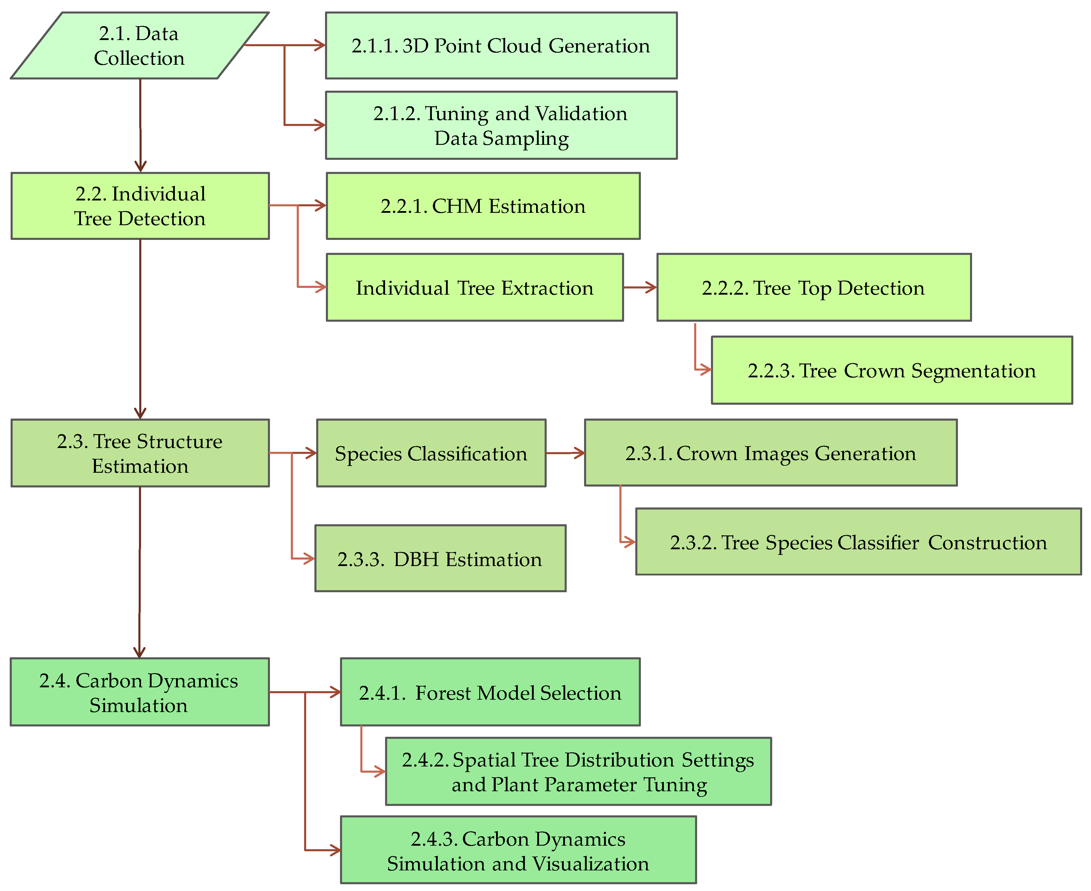
It is therefore highly desirable to develop an analytical process that seamlessly connects the understanding of high-resolution forest structure and the future forecasts of forest dynamics to support forest management in the field. Therefore, the purpose of this research is to develop an end-to-end process that enables the connection of the three processes seamlessly by combining digital images acquired by UAV and limited data from ground surveys: (1) The detection of individual trees via 3D point cloud data processing, (2) the estimation of forest structure via the use of empirical models and deep learning technology, (3) the prediction of future carbon dynamics.

2. Methodology

Figure 1 shows location of study sites. Two study sites were selected for the purpose of checking the applicability of the proposed end-to-end processes without depending on regional characteristics. Two study sites were located in Gifu prefecture, in the center of Japan (Figure 1a,b). The first study site (Site 1, 36.01° N, 137.37° E) is an artificial forest composed of conifers, which covers 0.81 ha, has an altitude of approximately 1000 m, and belongs to Takayama city in the northern part of Gifu prefecture (Figure 1c). The second study site (Site 2, 35.64° N, 137.48° E) is a 0.96 ha coniferous plantation at approximately 680 m above sea level which belongs to Nakatsugawa city in the southern part of Gifu prefecture (Figure 1d). The two sites are primarily composed of two species of tree; cypress (Japanese cypress, Chamaecyparis obtusa (Sieb. et Zucc.) Endl.) and cedar (Japanese cedar, Cryptomeria japonica (L. f.) D. Don). The dominant tree species is cypress at Site 1, and cedar at Site 2. The average age of the stands is 103 years in Site 1 and 47 years in Site 2. These study sites were selected because the forests that include these sites have been intensively thinned, rendering it feasible to accurately analyze the performance of the end to end process for this study.

The climate in the two study areas is humid subtropical, and hot and rainy in summer. The average rainfall is 1699.5 mm at Site 1 and 1746.8 mm at Site 2. The average temperature is −1.4 °C (Site 1), and 1.0 °C (Site 2) in January which is the coldest month; and 24.1 °C (Site 1), and 25.3 °C (Site 2) in August, the warmest month in the region. When taking the elevations of the two study areas into consideration, it is estimated that the temperature in the coldest month at Site 1 and Site 2 are −7.4 °C and −3.1 °C, and the temperature of the warmest month is approximately 18.1 °C (Site 1), and 21.2 °C (Site 2) respectively. For this study, aerial photography using an UAV was performed at Site 1 on 21 September 2016, and at Site 2 on 31 August 2017.

Figure 2 shows an overview of the end-to-end process developed in this study. The numbers in the flowchart correspond to the section numbers described in the text, and the details of each compartment are shown below.

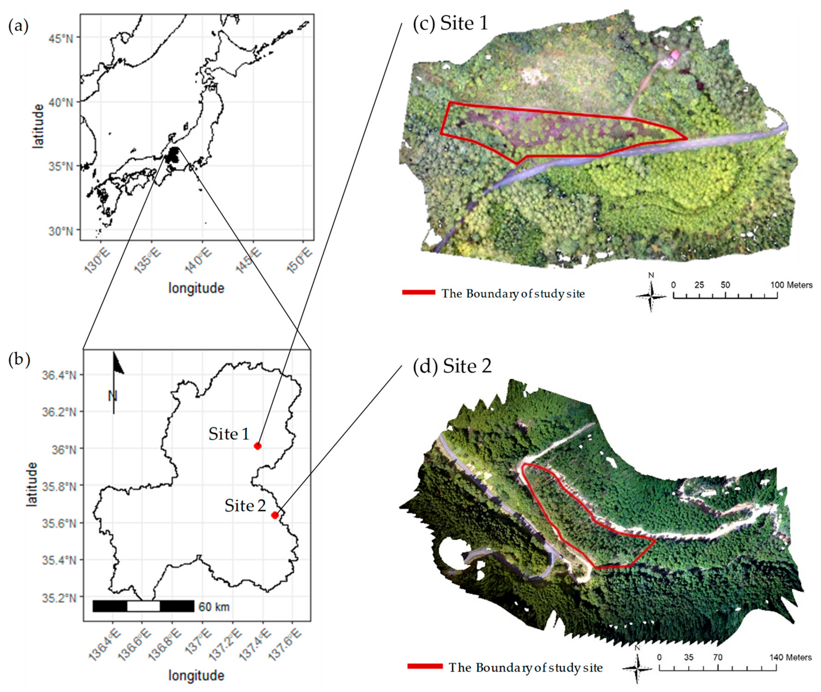
2.1. Data Collection

2.1.1. 3D Point Cloud Data Generation

From the aerial photography of the two target sites by UAV, 129 images of Site 1 and 152 images of Site 2 were acquired. 3D point cloud data was created for these images using the Structure from Motion (SfM) processing software (Photoscan Professional ver. 1.2.6, developed by Agisoft [44]).

Table 1. Settings used to generate 3D point cloud data.

Attribute		Site 1	Site 2
Number of images		129	152
Altitude of UAV flight	m	86.3	98.0
Ground resolution	cm/pix	3.11	2.27
Coverage area	km2	0.075	0.096
Tie-points		1,439,937	240,169
Error	Pix	0.417	0.494

shows the settings for taking and processing the data with the Photoscan software.

A DJI Phantom 3 Professional camera with 12 M pixels and a lens with a focal length of 20 mm (35 mm format equivalent) were used on the UAV for the survey of Site 1, and a DJI Phantom 4 Pro camera with 20 M pixels and a lens with a focal length of 24 mm (35 mm format equivalent) was used for the survey of Site 2. We used the Map Pilot for DJI software (developed by Drones Made Easy [45]) for the UAV auto-pilot.

2.1.2. Tuning and Validation Data Sampling

The DBH, coordinates, tree species, and tree height were measured for trees with a DBH of 0.05 m or more to collect data for the tuning and validation of the processes in Section 2.2 and Section 2.3 as described later in the text. The diameter (ACE) was used to measure the DBH, and a tree height pole (Senshin Kogyo, SK reverse scale inspection pole, AT-15) and laser ranging equipment (Nikon, Laser 550AS) were used for measurement of the tree height. The field survey was conducted at Site 1 on 1 November 2016, and at Site 2 from 31 October to 1 November 2017.

2.2. Procedure of Individual Tree Detection

2.2.1. CHM Estimation

Estimations of the tree and canopy heights were frequently performed for the creation of 3D point cloud data (Section 2.1.1) to ascertain the structure of the forest [46,47,48,49,50]. Tree height and canopy height are the basic properties that indicate the structure of a forest, and are important variables used for the estimation of other properties of forest structure such as the volume of timber and biomass [51]. Since this study estimates the height of single trees situated in coniferous forests on sloping mountains, it is necessary to estimate the CHM from the difference between the Digital Surface Model (DSM) and the Digital Terrain Model (DTM), as demonstrated in Equation (1):

$$CH{M}_i=DS{M}_i-DT{M}_i$$

(1)

where, i represents the index of the grid cell. The CHM was estimated from 3D point cloud data using the point cloud processing software FUSION (USDA Forest Service) [52] and ArcGIS ver.10.4.1 (ESRI) [53]. The detailed procedure was described with the applied software functions.

First, the points that were candidates for designation as ground surface points were extracted from the 3D point cloud data, and were re-gridded onto grid cells with a resolution of 1.0 m. The height of the lowest point in each grid cell was extracted as the ground surface height for the grid cell (FUSION: ground filter function). However, it is well known that these points often contain errors and the surfaces of tree-crowns are often mistaken for the ground surface during the process of creating the 3D point cloud data. Therefore, grid cells with a resolution of 1.0 m were re-gridded onto grid cells with a resolution of 0.5 m, the height of each grid cell was estimated by extrapolation, and outliers were removed by spike processing. A smoothing function was then applied using the median filter to estimate the DTM (FUSION: GridSurfaceCreate function). Since the accuracy in the estimation of the DTM depends on the size of the median filter the size of the filter was determined via exploration. Finally, the DTM was re-gridded onto a grid cell with a 0.1 m resolution by extrapolation and the highest point within the grid cell, i, was set as the DSM of the grid cell i. The tree height model CHM in grid cell i was then determined from the difference between the DSM and the DTM (FUSION: CanopyModel function).

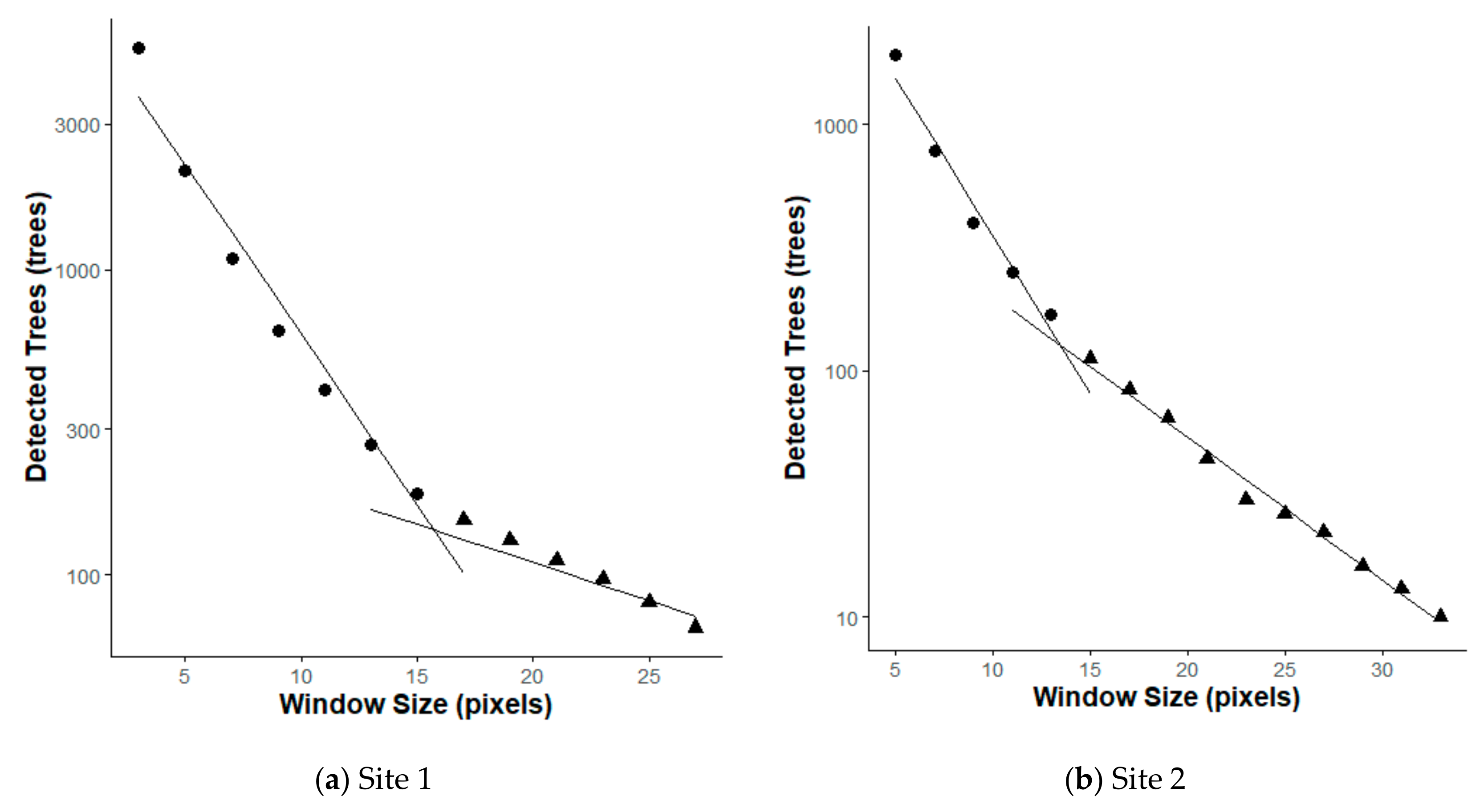
2.2.2. Tree Top Detection

The CHM created in Section 2.2.1 is usually used for various purposes such as tree top detection, crown shape visualization, and the estimation of tree volume [34,35,36,37]. Many other methods have been applied to tree top and crown extraction using CHM. Examples include local maxima detection algorithms for tree top extraction, the valley following method, the region growing method, the concave hull method, and the watershed method for tree canopy segmentation and drawing [31,54,55,56,57]. The method detecting the maximum value is thought to be suitable for this study because conifers such as cedar and cypress have a conelike shape and the difference between the apex height and height of the periphery part is clear. rLiDAR ver. 0.0.1 [58] was used to analyze and visualize the LiDAR datasets in this study. The detailed operations are described below, together with the software functions that were used.

Tree tops were automatically detected using the CHM and the Local maxima method (rLiDAR: FindTreesCHM function). This function is based on the local maximum search method and detects treetops by sequentially searching the moving window in the CHM by using a fixed tree top window size, the Fixed Window Size (FWS) in the CHM. In order to find the optimal number of treetops, the number of treetops was searched for after smoothing the CHM with a Gaussian filter (rLiDAR: FindTrees CHM function, CHMs smoothing function). The optimal FWS was then determined by changing the FWS from 3 × 3 to 33 × 33 in 2 pixel steps and detecting the elbow points.

2.2.3. Tree Crown Segmentation

Next, a new crown segmentation function based on the watershed method was introduced. The crown segmentation function that was originally implemented in rLiDAR was based on a centroid Voronoi approach (rLiDAR: ForestCAS function). Gravity Voronoi segmentation is a method based on the distance between target points and the target points in this research was the treetops. When Gravity Voronoi segmentation is used, it is possible to separate tree crowns by taking into consideration the positional relationship of the treetops, but it is not possible to determine the size of a tree crown by considering different tree heights according to tree growth stage. The watershed method was therefore used in this study to consider the difference in the height of each tree in addition to the distance between treetops. The threshold for the lowest tree height was set at 8.0 m in order to avoid the misdetection of forest undergrowth and rocks as trees. In addition, the threshold for maximum crown radius was set at 5.0 m, according to the empirical information collected during the field survey, and the CHM was divided into individual crowns by the function using the watershed method (cf. rLiDAR: ForestCAS function).

2.3. Tree Structure Estimation

Using the information concerning the individual crowns segmented in Section 2.2.3, a method for the identification of tree species was developed by extracting the features of a 3D tree-crown shape and leaf foliation.

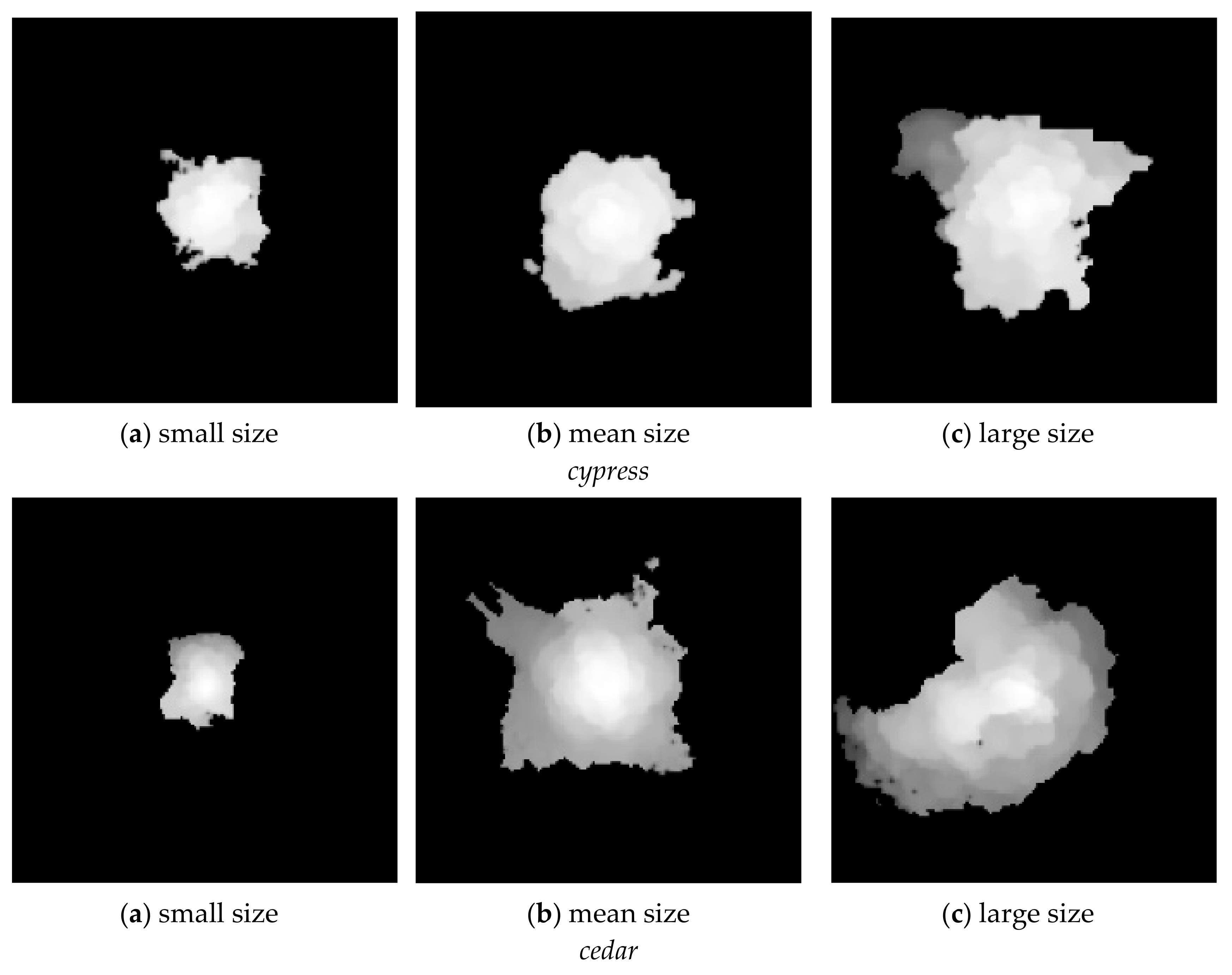
2.3.1. Crown Images Generation

A classification method for the identification of tree species was constructed by focusing on the difference in the 3D shapes of the separated crowns as in Section 2.2.3, which depends on the tree species. From the results of the segmentation into individual tree crowns, planar images representing the 3D shape of the crowns were created with a resolution of 10 cm. First, a pixel representing a treetop was set at the center of an image. All pixel values in each image were then scaled in 256 steps so that the pixel value of the tree was 255 and the ground surface was zero. Finally, gray scale images of 161 × 161 pixels (one pixel is 10 × 10 cm) were produced which could represent a crown radius of 8.0 m, which was the maximum crown radius detected at the target site. Data from the trees surrounding Site 2 were added to increase the amount of data used for the development of the tree species classification system. The individual tree was detected using the UAV aerial image of the neighboring stands according to the method described in Section 2.2, and the tree species was determined visually using the point cloud visualization software Bentley Pointools View ver. 02.00 [59].

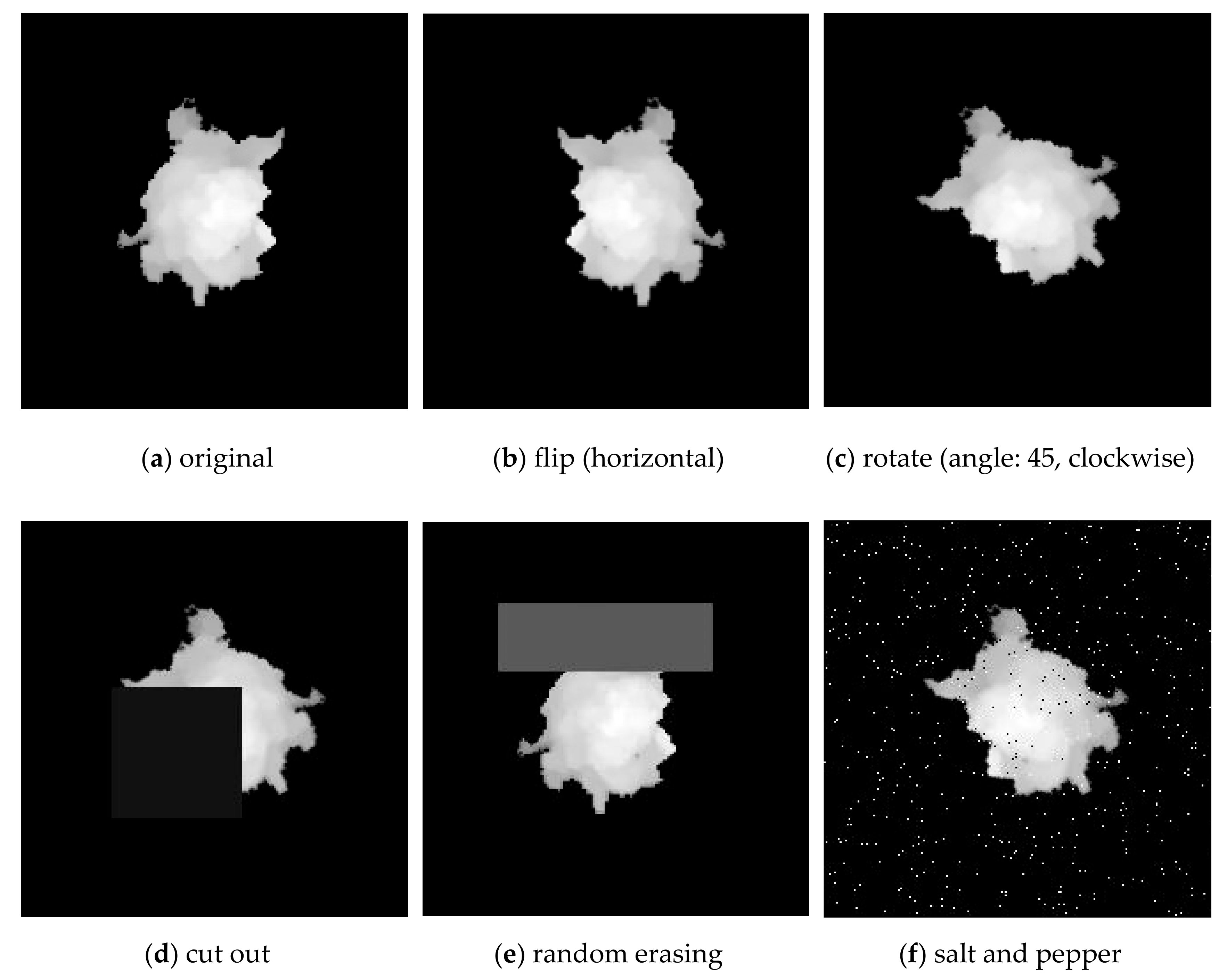
2.3.2. Tree Species Classifier Construction

The total dataset of the crown images was divided into 90% and 10% for the training and verification data set, respectively, and the performance was evaluated with 10-fold cross validation. ResNet-200 [60], which is a convolutional neural network architecture with high accuracy but high calculation cost, was selected as the framework for deep learning because of the prioritization of identification accuracy within the system. The parameters for the model training are given in

Table 2. The settings of the Image Classification Model.

Setting	Selected Option
Training epochs	10
Batch size	64
Base learning rate	0.01
Solver type	SGD
Network	ResNet-200

. Mxnet [61] was used as the framework for the implementation of the deep learning-based identifier. Fine-tuning was performed by setting the network weights pre-trained in the 1000 classification task of ImageNet [62,63] as the initial values.

Data augmentation was applied to the crown images for the model training process. The purpose of data augmentation is to increase the number of crown images and to construct a robust classification system corresponding to the various shape of the crowns [64,65]. The five types of data augmentation applied in this research were: (1) Rotation, (2) Flipping, (3) Cutout, (4) Random Erase, and (5) Salt and Pepper. In the (1) Rotation process, a crown image was rotated clockwise by 15 degrees, ranging from 15 to 330 degrees around the treetop. For (2) Flipping, crown images were flipped horizontally and rotated in the same way as above. These augmentations can contribute to an increase in the general performance due to the different directions of the trees. The (3) Cutout [66] and (4) Random Erasing [65] methods are used for cropping a part of the image. In the (3) Cutout process, a crown image was cropped using a square mask and the cropped pixels were padded with an average value over the entire image. In (4) Random Erasing, a crown image was cropped by masks with various aspect ratios and the values of the cropped pixels were padded with a random value. These techniques can improve the performance of the identification of the crown images which was partially lacking in the crown segmentation process. In the (5) Salt and Pepper process, 1.0% of the pixels of a crown image were randomly selected and each pixel was filled with random values from 0 to 255. This was expected to mitigate the errors and outliers often included in 3d point cloud data. Using these augmentation processes, 192 crown images were generated from a single crown image. Finally, all the crown images were resized to 224 × 224 pixels and the pixel values were copied to three channels.

2.3.3. DBH Estimation

In addition to tree height, the DBH has often been used as an important parameter to estimate elements of the forest structure such as volume and biomass [67,68]. However, DBH cannot be obtained directly from the 3D point cloud data acquired by LiDAR or UAV, so a new method is needed to estimate the forest structure. Since highly accurate tree height and crown dimensions can be obtained, an estimation of DBH was often attempted using these parameters. The method for DBH estimation using tree height and crown diameter has a particularly high accuracy [67,69]. In our study, the tree height and crown diameter were estimated from the individual crowns segmented by the process described in Section 2.2.3. and Equation (2) was applied to estimate the DBH [67].

$$D=0.557\times {\left(H\times cr\times 2\right)}^{0.809}\times exp\left(\frac{{0.056}^2}{2}\right)+\alpha$$

(2)

where D is DBH in meter unit, H is tree height in meter unit, cr is crown radius in meter unit, and α is a correction term for the tree species in Equation (2). The H and cr were computed using the heights and ground-projected canopy area (rLiDAR: ForestCAS method), respectively. Although Equation (2) had been proposed as a general allometric model by analyzing global database of more than a hundred thousand trees [67], the correction term α was derived from the sample data acquired in the field survey of Section 2.1.2, to consider systematic errors included in the 3D point cloud data. We calculated root mean squared error (RMSE) between observed DBH and calculated DBH which includes the α parameter and minimized the RMSE by optimizing the α parameter.

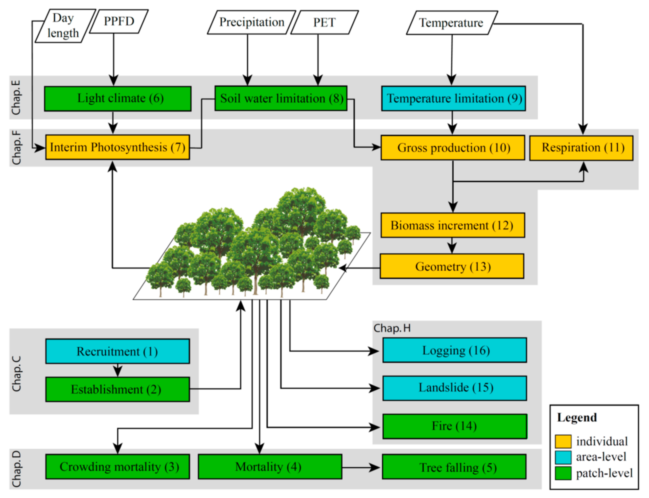
2.4. Carbon Dynamics Simulation

The process for the future simulation of the carbon dynamics of single tree units using tree crowns as detected in Section 2.2, tree species, and estimated crown parameters identified in Section 2.3 is described below.

2.4.1. Forest Model Selection

We used an individual and process-based forest gap model, FORMIND v3.2 [40]. This version of FORMIND is suitable for our process because (1) an initial state derived by UAV observation can be input into the model, (2) the model can simulate carbon dynamics at an individual tree level which provides useful information for forest management, and (3) the model can simulate forest management options and accurately visualize the effects. Figure 3 illustrates an overview of the FORMIND model. The FORMIND model can be applied at a local scale (several hectares), on forests which consist of multiple species of tree at different stages of growth [70,71]. The model has four main processes: (1) Recruitment and establishment, (2) mortality, (3) competition and environmental limitations, and (4) the growth of a tree. The growth of a tree is computed by considering photosynthesis, respiration, and geometry such as stem diameter, height, crown diameter, crown length, and the crown projection area. The photosynthetic production is computed using the availability of light. Study sites are divided into patches of 20 m resolution. A tree species competes with the other trees on the same patch. The FORMIND model can simulate above- and belowground carbon stock and flux by considering forest management, and the model can be utilized for scenario analysis in forestry practices [72,73].

2.4.2. Spatial Tree Distribution Settings and Plant Parameters Tuning

The FORMIND model requires (1) coordinate data, (2) species name, and (3) the DBH for each tree. The coordinate data for all tree species at a resolution of 0.1 m was used, as identified in Section 2.2 (see Section 2.2.1, and Section 2.2.2). The species of the individual trees was identified according to class, with a higher probability of cedar and cypress using the classification system for tree species constructed in Section 2.3.2. The DBH of the individual trees was estimated using the allometric equations developed in Section 2.3.3.

The FORMIND model represents tree species as plant functional types (PFT). Parameters for DBH growth and shade tolerance should be calibrated for each PFT. The model has been applied to tropical rain forests in Africa and South America [39,71,74]. However, there are few applications recorded in temperate coniferous forests and the growth parameters for cedar and cypress have not been reported [75,76]. Therefore, we calibrated the curve for the maximum growth diameter, the gross photosynthetic rate, the height-stem diameter relationship, and the aboveground biomass-stem diameter relationship by using empirical relationships between forest age and tree heights, DBH, basal area, and stem volume [77]. The calibrated parameters are given in Appendix A.

2.4.3. Carbon Dynamics Simulation and Visualization

We visualized plausible future carbon dynamics from the following three viewpoints by simulating changes in the carbon stocks of the forest ecosystem and for each tree from 2018 to 2100. (1) In terms of growth management and the plans for harvesting individual trees, we tracked the spatial distributions of the stem volume and tree height and monitored the competition within the stands. (2) From the viewpoint of supporting a sustainable and efficient plan for the harvesting of the trees, we estimated the changes to the aboveground biomass and the expected yields. (3) In the light of supporting the MRV of carbon dynamics in REDD+ [78], we visualized the changes in the carbon in the above-and belowground biomass, soil, and dead wood. The patch size and time steps were set at 20 m and one year, respectively. Thinning was not simulated because any thinning based on the regional standard forestry plan for operation has already been completed at both of the target stands. Natural regeneration was also excluded because we assumed the regular cutting of underwood.

3. Results

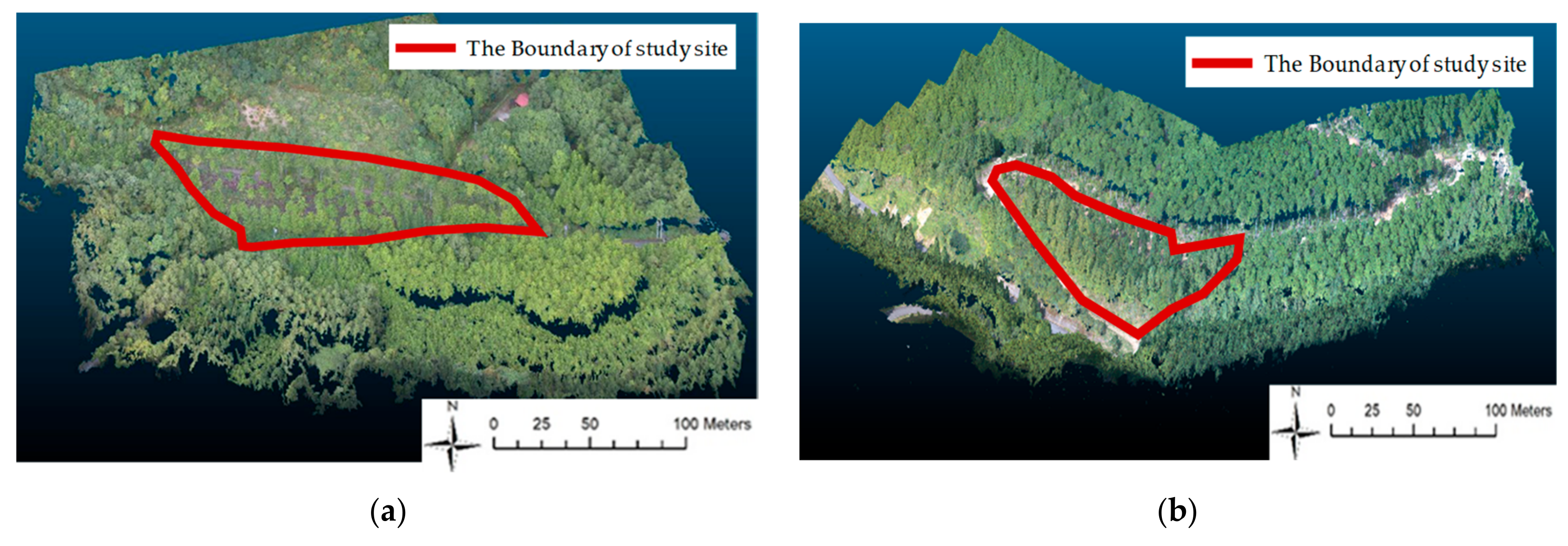
3.1. Data Collection

3.1.1. 3D Point Cloud Data

The orthographic images and 3D point cloud data were created via UAV-SfM using Photoscan by inputting an aerial image taken by the UAV are shown in Figure 1c,d and Figure 4. The areas bounded by red lines were the target sites. The camera position and the overlaps are shown in Figure 5. The overlap in photo coverage area was 90% in a forward direction and 85% in the cross direction at both sites. Photos were taken in DNG format and were processed using PhotoScan [44].

3.1.2. Tuning and Validation Data

In the field survey, 115 cypresses and 22 cedar trees were observed at Site 1, and 27 cypresses and 182 cedar trees were observed at Site 2. The details of tree type, DBH, and tree height are shown in

Table 3. Summary of Field survey.

Species	Attributes		Site 1				Site 2
			N	Min	Max	Mean	N	Min	Max	Mean
cypress	DBH	m	115	0.125	0.454	0.324	27	0.169	0.302	0.230
	Tree Height	m	25	20.8	27.0	24.1	18	14.6	24.0	18.7
cedar	DBH	m	22	0.163	0.374	0.238	182	0.173	0.509	0.283
	Tree Height	m	5	15.0	26.7	22.5	93	14.0	26.8	21.6

for each site. In both target areas, there were some areas that could not be accessed due to topographical conditions, but approximately 60% and 80% of the trees were observed in Site 1 and Site 2, respectively. The numbers of DBH and tree height were different due to the limitation of field survey resources.

3.2. Individual Tree Detection

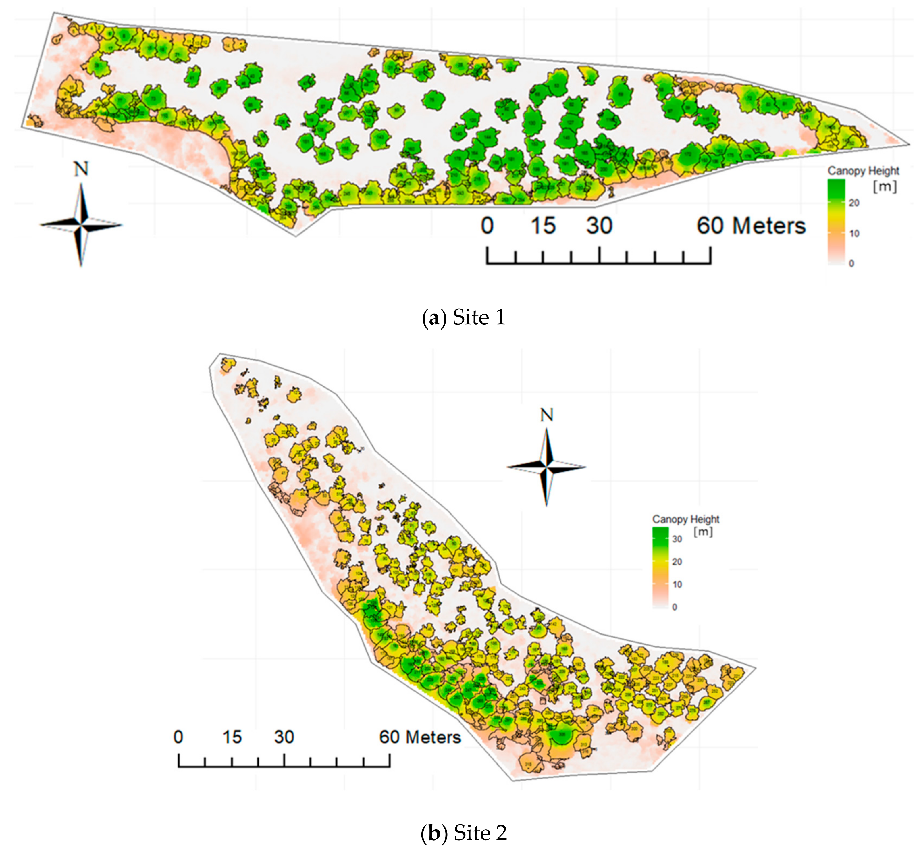
3.2.1. Estimated CHM

Figure 6 shows the DTM for each site estimated from the 3D point cloud data created in Section 3.1.1. In the southeastern part of Site 1, Figure 6a crown height was mistakenly estimated as the same as the height of the ground surface in the south east region of the original DTM, but the overestimation of the DTM was modified by smoothing using spike treatment and median filter as demonstrated in Figure 6b. In the southwest part of Site 2, many local pitfalls that were not actually present were generated in Figure 6c; these local holes were removed by applying the same smoothing as shown in Figure 6d. The window sizes of the median filter were tuned to 2.1 m at Site 1 and 1.5 m at Site 2 by comparing the measured and estimated maximum tree heights at each site.

Figure 7 shows the estimated CHM produced by calculating the difference between the DSM and DTM according to Equation (1) and based on the 3D point cloud data created in Section 3.2.1. At both sites, the crown boundary was clearly detected in areas of low stand density, but the crown boundary tended to be unclear in high density areas. In the western part of Site 1 in Figure 7a, the forest density was high because thinning had not been performed due to topographical constraints. Therefore, the DTM could not be accurately estimated, and this affected the accuracy of the estimation of CHM. At Site 2 in Figure 7b, tree height was also overestimated in the southwest region compared to that actually measured despite the smoothing of the DTM. This error may have occurred because the model estimated a shallow DTM slope in this area, while the actual slope in the southwest observed in the field survey was very steep.

3.2.2. Extracted Individual Tree

Figure 8 shows the relationship between the size of the tree top search window (FWS) and the number of treetops detected from the CHM. The number of detected treetops depended on the FWS, and elbow points were observed for both Site 1 and Site 2. While the small projections in the individual crowns are erroneously recognized as treetops with small FWS, large FWS tend to regard multiple peaks as a single tree crown. Segmented regression [79] was applied by using segmented regression package [80] on R ver. 3.5.3 [81] to determine the elbow points which could decide the suitable FWS and the number of treetops detected. 15 pixels (1.5 m) at Site 1 and 13 pixels (1.3 m) at Site 2 were selected as representatives for the FWS. The size of the Gaussian filter was tuned to 11 × 11 at Site 1 and 13 × 13 at Site 2 by comparing the observed number of trees and the estimated number of treetops.

Figure 9 shows the images of the detected treetops after smoothing the CHM with a Gaussian filter, and

Table 4. Tree detection rate on both sites.

		TP	FN	Recall
cypress	Site 1	107	8	0.93
	Site 2	27	0	1.00
cedar	Site 1	16	6	0.73
	Site 2	169	13	0.93

TP: True Positive, Detected by both field survey and model. FN: False Negative, Detected by field survey, but not detected by model. Recall: TP/(TP + FN), Proportion of actual positives was identified correctly.

summarizes the accuracy of the results for individual tree extraction with the optimized tree top search filter. The percentage of individual trees detected using this model was 94.4% cypress and 90.7% cedar, thereby achieving an average overall detection rate of 92.3%. However, there were some errors. At Site 1, strong thinning was carried out in 2015 except for in the western area where the topography is steep. Since the ground was hidden by density of tree crowns in this area, it was difficult to observe the ground surface from the aerial image taken by the UAV. As a result, the GridSurfaceCreate function mistakenly regarded the crown surface as the ground surface in the DTM estimation process, meaning that the CHM was extremely small and the tree could not be detected. Errors also occurred at Site 2 in constructing the 3D point cloud data from the aerial data taken by UAV for unknown reasons. Compared with the field survey, the 3D point cloud for the northwestern part was partially missing and the number of points was insufficient. The height of the 3D point cloud near the ground surface in the southwestern area was created underground in part of the point cloud, showing an abnormally low height in the DTM, and over splitting occurred. These errors caused the generation of numerous very small crowns and unusually large crowns at Site 2.

3.3. Tree Structure Estimation

3.3.1. Species Classifier

Figure 10 shows examples of the individual crown images as separated in Section 3.2. 326 cypress and 265 cedar were acquired as the dataset for the training and validation of the tree species classification system. The images of cypress and Japanese cedar crowns had radii of 0.70–7.28 (mean = 3.95, s.d. = 1.08) and 0.22–9.44 (mean = 3.33, s.d. = 1.29), respectively.

Examples of augmented crown images for training data are shown in Figure 11. Figure 11a is an original crown image. By horizontally flipping the original image of Figure 11a, as shown in Figure 11b, the number of images was doubled. Each image was rotated by 15 degrees as shown in Figure 11c, resulting in 48 images. Each augmentation method—Figure 11d cut out, Figure 11e random erasing, and Figure 11f salt and pepper—was also applied to each image. An original crown image was thereby augmented to 192 images. As a result, 102,124 training images and 59 validation images became available for each cross validation process.

Table 5. Classification result by ResNet-200.

		Reference		N	Precision
		Cypress	Cedar
Prediction	cypress	279	50	329	0.848 (0.01)
	cedar	47	215	262	0.821 (0.01)
	N	326	265	591
	Recall	0.856 (0.01)	0.811 (0.01)		Overall Accuracy
	F-value	0.852 (0.01)	0.816 (0.01)		0.836 (0.01)

TP: True Positive, Detected by field survey and model. FP: False Positive, Detected by model, but not detected by field survey. FN: False Negative, Detected by field survey, but not detected by model. Recall: TP/(TP + FN), Proportion of actual positives identified correctly. Precision: TP/(TP + FP), Proportion of trees detected by model positives were also correctly detected by the field survey. F-value: 2 * Recall * Precision/(Recall + Precision), harmonic average of the precision and recall. Values of Recall, Precision, F-value are mean and values in round brackets show the standard error of the 10-fold cross validation.

shows the confusion matrix for the results of the 10-fold cross validation. The overall accuracy was 83.6%. F-values were over 80% and slightly better for cypress than cedar. Since cypresses were the predominant inhabitants of Site 1 where the stand density is low due to thinning, the classification system could be learned using well segmented crown images. It is further thought that the division accuracy of the crown image influenced the classification accuracy because Japanese cedar inhabited site 2 with a high stand density, which made it difficult to identify individual trees.

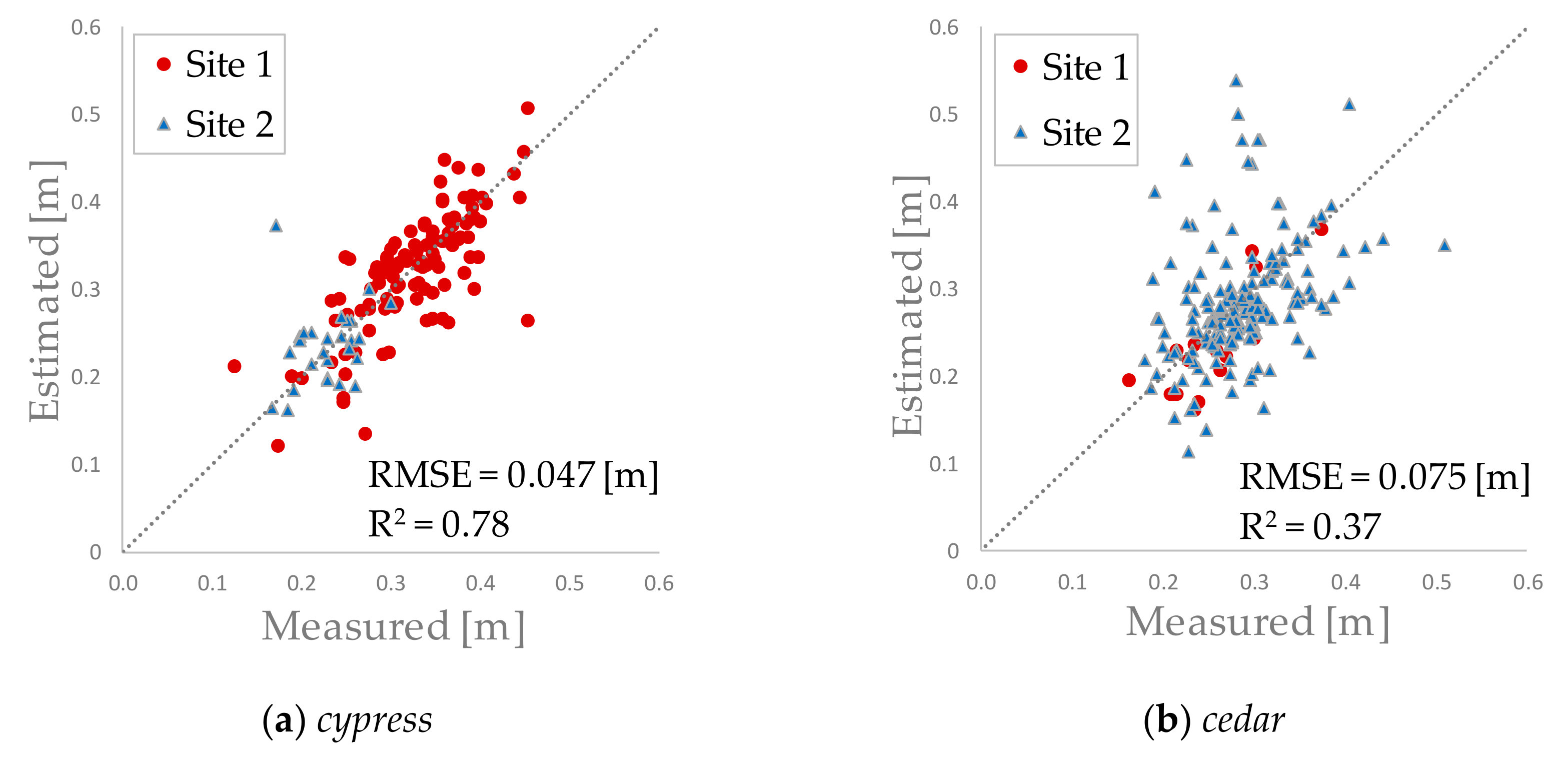
3.3.2. Estimated DBH

Figure 12 is the comparison of the DBH estimated using Equation (2) and the observed DBH obtained in the field survey, using the estimated tree height as in Section 3.2.2 and the estimated crown diameter from Section 3.2.2. The correction term α of Equation (2) was set at 0.070 for Japanese cypress and 0.092 for Japanese cedar due to the minimization of the RMSE compared with the field survey results. A good estimation was obtained for the cypress at both Site 1 and Site 2. In contrast, there were relatively large errors at Site 2, which is dominated by Japanese cedar. The cause of this could be that the crown diameter was obtained from over-division and the abnormally shaped crowns of Site 2. One of the ecological characteristics of cedar is that it avoids contact with adjacent trees, branches, and leaves [82]. As the average crown sizes were 3.82 m at Site 1 and 3.07 m at Site 2, the growth of the crown may be limited at Site 2 due to the high stand density.

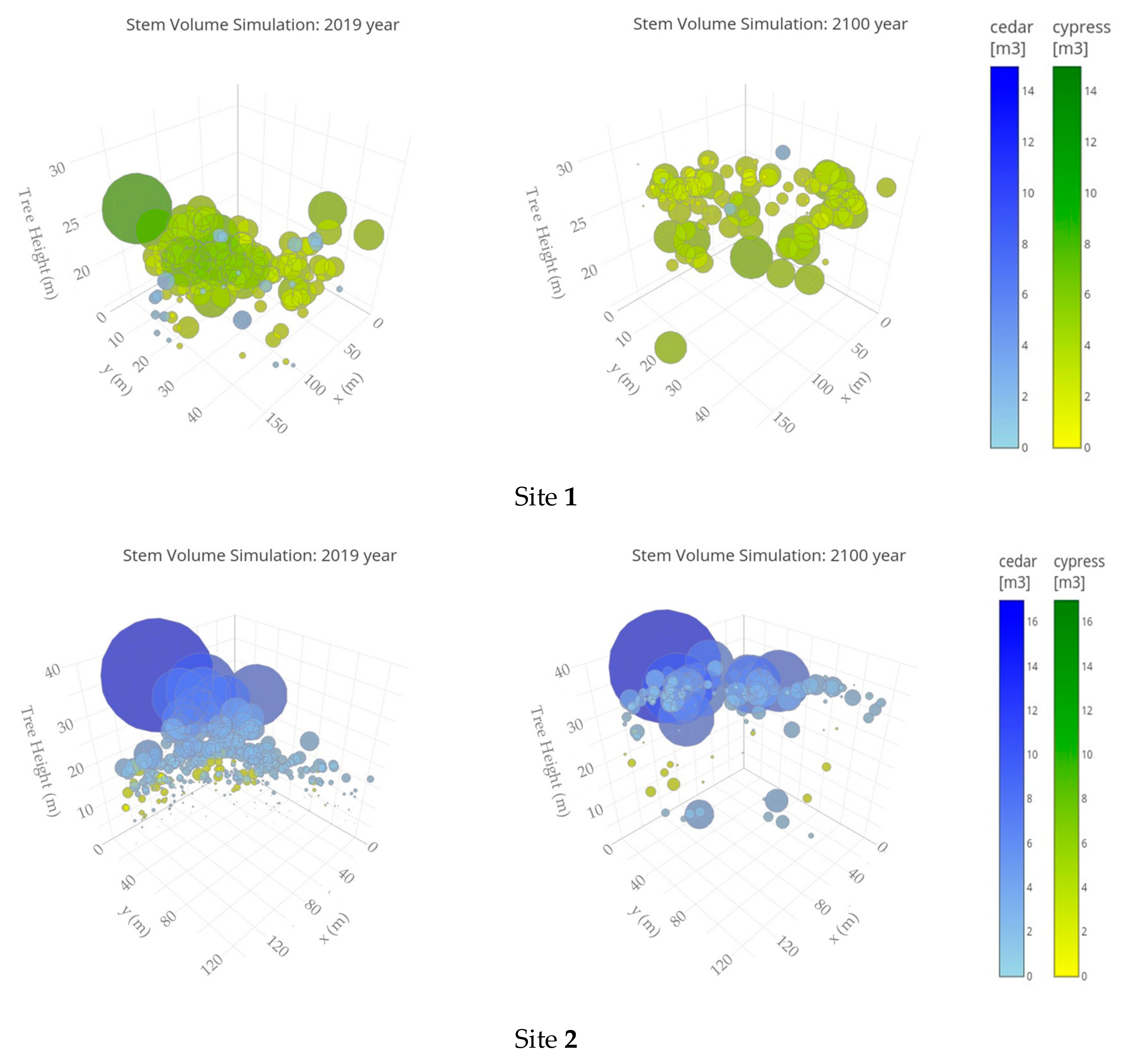
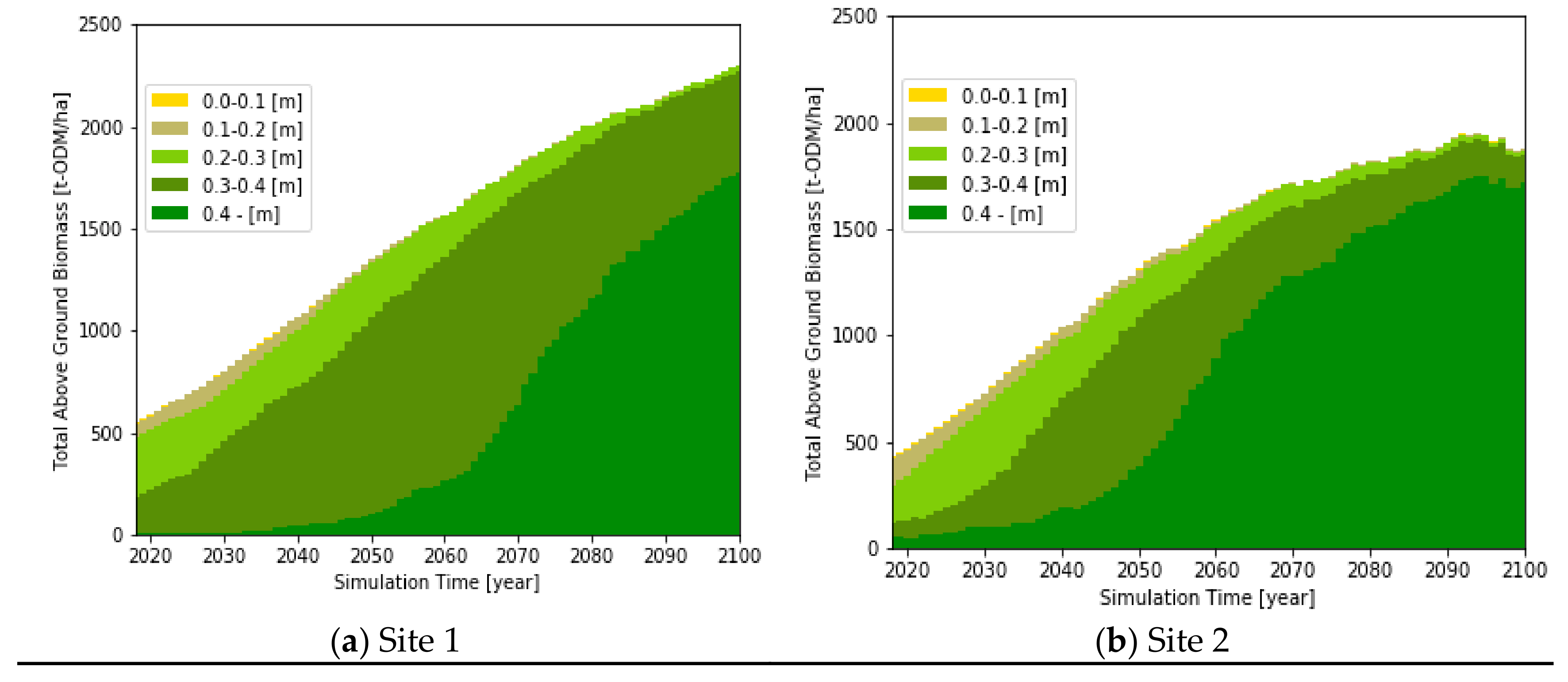
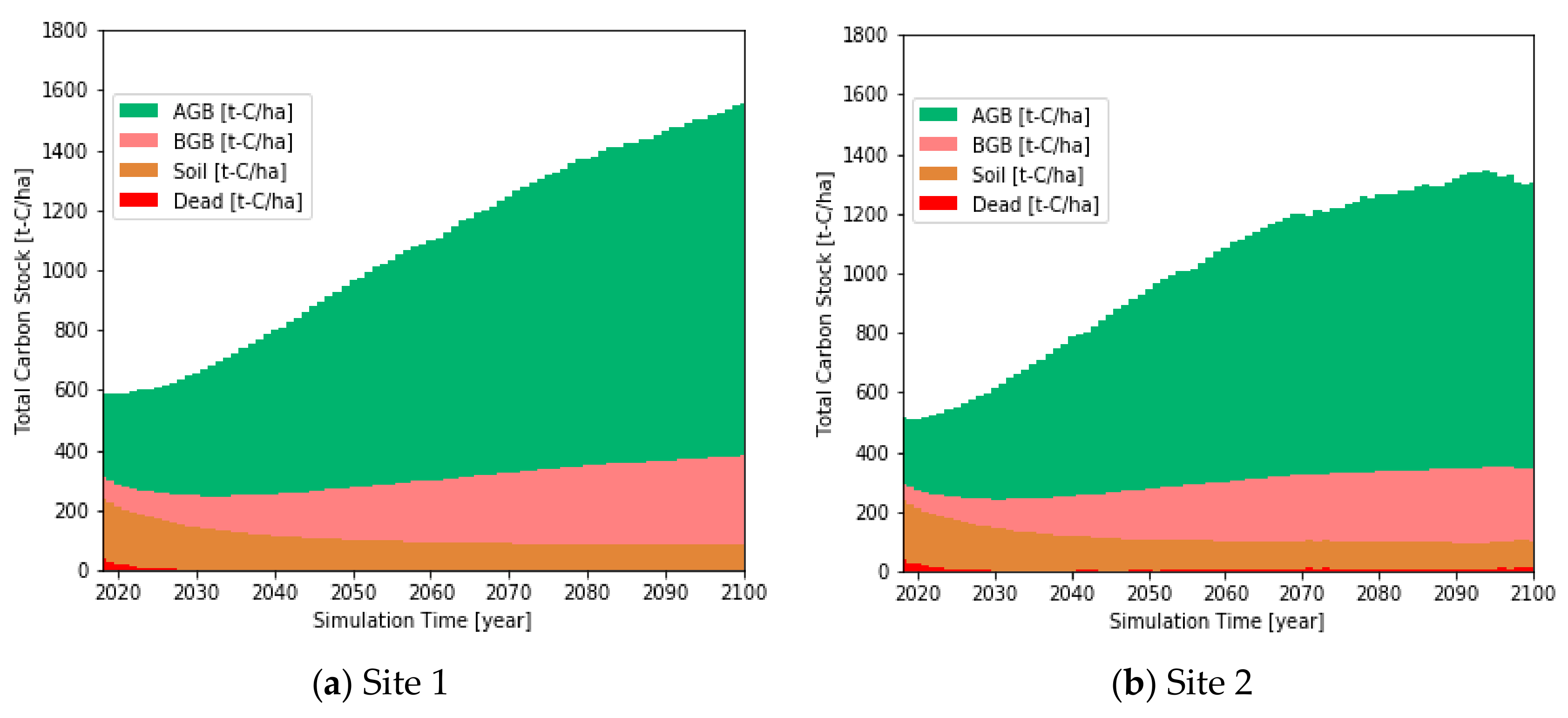
3.4. Carbon Dynamics Simulation

Figure 13 and

Table 6. The results of carbon stock simulation. Values for DBH, tree height, and stem volume represent mean values within the sites. Values in brackets denote standard deviations.

		Site 1		Site 2
		2019	2100	2019	2100
Number of Trees	trees	263	214	319	164
cypress		169	133	57	20
cedar		94	81	262	144
Density	trees/ha	325	264	332	171
DBH	m	0.19 (0.09)	0.42 (0.07)	0.17 (0.08)	0.43 (0.04
Tree Height	m	16.2 (5.84)	29.6 (4.07)	15.3 (6.08)	30.5 (8.16)
Stem Volume	m3	1.51 (1.54)	8.12 (2.80)	1.09 (1.47)	9.25 (4.34)

show the spatial distributions of individual trees in 2019 and 2100 and the stand structure, respectively. The inter-tree competition reduced the tree densities at each site by 19% and 48%, respectively. The mean DBH increased by 2.2 and 2.5, the mean tree heights increased by 1.8 and 2.0, and the mean stem volume increased by 5.4 and 8.5 times, respectively. This result shows that both target sites have the capacity to grow in terms of biomass by 2100. This information at an individual scale enables us by helping to decide which trees should be cut at high resolution.

Figure 14 and Figure 15 show the changes in aboveground biomass by DBH size class, and carbon stock by components, respectively. The AGB at site 1 was still increasing in 2100, while the AGB at site 2 indicated a state of equilibrium by 2090 (Figure 14). In 2019, site 1 was dominated by trees with a DBH class of 0.2–0.4 m. The DBH size of the dominant trees increased over the duration of the simulation. Site 2 was mainly occupied by trees with a DBH class of 0.2–0.3 m in 2019. However, the DBH size increased rapidly compared with site 1 and the biomass reached equilibrium. In terms of the carbon stocks, at site 1, the carbon in above- and below-ground biomass was still increasing in 2100 (Figure 15). However, all the components at site 2 had reached a state of equilibrium by 2090. Therefore, site 1 can still absorb CO₂ after 2100, even though site 2 has limited ability. The results of the simulation of AGB by DBH class and carbon stocks by components enables us to consider the usage of timber. Therefore, our simulation results can be used for planning forest management, taking into consideration the demands for timber or biomass energy and the effects of carbon sequestration.

4. Discussion

4.1. How to Improve the Accuracy of 3D Point Cloud Data

For the process of image data acquisition, basic improvements can be made, such as using the latest drones with high resolution cameras, optimizing the flight path and altitude, improvements to dpi and the fps of images, and selecting the best conditions for weather and insolation. The accuracy of the data can also be improved by setting an additional Ground Control Point (GCP). The use of a drone carrying Real Time Kinematic (RTK) to upgrade the quality of the images and point measurement would improve the images. Another consideration here is whether images should be taken from a constant altitude above ground level.

The quality of 3D point cloud data at Site 2 was found to be low when carrying out the process of generating 3D Point cloud data. This was because Site 2 was located on a steep slope, meaning that the number of reference points was limited due to the difficultly of the GCP setting. The detailed reason is not yet clear, but possible reasons were that Site 2 is located on the steep valley, or that the forest is young and thinned. We could not undertake RTK measurement in the forest due to the multi-path, but the accuracy might be improved by measuring the GCP directly by a surveying technology, such as, total station.

Finally, in the validation data sampling process, we validated the estimation for the location and the DBH of individual trees in the field survey. However, the results are thought to have uncertainties due to the measurement of large trees in extremely dense forests. Errors in the GPS coordinates for both the UAV and digital camera could also have affected the accuracy of the evaluation. This might be mitigated by introducing the latest high-resolution devices such as drones with Post Processed Kinematic [83] or the Quasi-Zenith Satellite-1 “MICHIBIKI” [84], which have fine resolution at the centimeter level.

4.2. Individual Tree Detection and Issues

In the process of estimating the CHM from 3D point cloud data (in Section 2.2.1), 3D point cloud data was repeatedly re-gridded and filtered using processes such as the ground-filter function of FUSION or the gridsurfacecreate function [52] to remove spikes and outliners and to estimate the DTM. The conversion processes rendered the original 3D point cloud dataset in centimeter resolution upscale to meter resolutions. This upscaling may lose useful information for the detection of trees and the identification of species. Grid cell size was empirically decided. The cell size may affect the performance, so a systematic parameter tuning process using grid search or Bayes optimization should be implemented.

In the process for the detection and separation of the treetops (in Section 2.2.2), an overall detection rate of 92.3% was achieved for the tree crowns. This performance was good compared to the 85% rate of detection in previous studies using UAVs [57]. Good detection rates were achieved for cypress at both sites, but Japanese cedar had a low rate of detection, particularly at Site 1. The first plausible reason was that the cedar trees were young and of lesser average height than the cypress. It has been reported that small trees were not detected as they were surrounded by adjacent tall trees [85]. Research using LiDAR data and the Watershed method reported that that the higher density of crowns, the lower the detection performance, even in the same forest [86]. One solution may therefore be to evaluate the crown density in the searching process and vary the window size according to the density, for example by using a window of small size where a stand of high density is investigated. In addition, the search range for the window size was determined empirically by trial and error during the segmented-regression process used to determine the window size for the detection of treetops in this research. One of the plans for improvement is to use techniques such as data assimilation to determine the size of the window by referring to and reproducing the number of trees observed in the field survey.

4.3. How to Improve the Accuracy of Species Classification

Among the crown images used for the development of the classification system, particularly at Site 2 which includes the steep slope area, images with an abnormal shape such as that shown in Figure 16 were confirmed in the generation of the crown image generation (in Section 2.3.1). Figure 16a has a crown radius of 2 pixels (20 cm) and showed an abnormality in the allometry with DBH. The tree crown was only partially detected in Figure 16b. Figure 16c was divided by a straight line at the boundary with the adjacent crown, and there was no part where the crown vertically overlapped. Figure 16d was a candidate for a tree that was found on a steep slope and the ground surface and the canopy were combined by mistake. Since mixing these with learning data might affect the learning and validation performance, it is necessary to establish rules for exclusions from the learning data.

Although the height distribution of the crown shape was expressed by a 2D image in this study, several image creation methods exist to express the features of a tree crown. For example, [87] achieved 86.1% accuracy with 10 different tree species in the Deep Boltzmann Machine using the cross-section images of the road tree acquired by Mobile LiDAR. Thus, the identification of tree species using the height distribution of a tree crown is considered to be effective. [88] used spectral information to classify four types of tree species in addition to the structural features of tree crowns acquired by UAV using multi-layer perceptron. This achieved an accuracy of 95.2% and the infrared spectrum was found to be effective for the classification of conifers such as Birch. Furthermore, [38] identified tree species such as evergreen broad-leaved trees, deciduous coniferous trees, and pine using only color information from ortho images acquired by UAV. Augmentations such as rotation, scaling, shear strain were applied to the crown images and achieved a performance of 89.0%. The classification accuracy can be expected to be improved by suppling multimodal information.

4.4. Application for Carbon Dynamics Simulation

This study developed an end-to-end process to simulate the future state of stand volume, carbon stock in the forest ecosystem, and forest attributes by coupling the current forest conditions derived by UAV with an individual-based gap model. Scenario analysis and a multidimensional evaluation of forestry practice is required.

Scenario analysis considering climate change is essential for forest management to support climate change mitigation and adaptation. The Ministry of Agriculture, Forestry and Fisheries in Japan is planning to implement eco-friendly management options under conditions of depopulation such as long rotation forestry or the conversion from conifer plantation to broadleaf forests [89]. The simulation results of the FORMIND model can be translated into the amount of timber produced. Thus, forest managers can test the feasibility of management scenarios. This information can support forest management in terms of the appropriate use of biomass resources and the management of biosphere carbon stock.

The simulated information for forest attributes can be used to evaluate not only carbon dynamics but also biodiversity and ecosystem services. For example, forest landscape modelers are trying to visualize the future forest landscape under climate change scenarios by coupling simulation results for forest succession with immersive virtual reality techniques [90]. Visualizing the future landscape helps us understand the recreational and cultural ecosystem services which affect decision making in forest management. Other ecosystem services can be evaluated via changes in land cover and ecosystem functions simulated by the FORMIND model, as in the case of research covering large areas [91,92]. In addition, outputs form simulation models can be used to estimate the extent of habitats available for wildlife [93]. In Japan, the conservation of rare wildlife species and the management of harmful animals are key concerns. Our process is also capable of connecting to existing habitat suitability index models and expert knowledge which requires detailed information concerning forest attributes.

5. Conclusions

In this study, we proposed a novel end-to-end process coupling UAV-derived 3D point cloud data with limited ground survey data, which included (1) individual tree detection, (2) tree species classification and (3) carbon dynamics simulation using deep learning technology and a process-based simulation model. We targeted two coniferous forests, mainly consisting of Japanese cypress and cedar. First, to detect individual treetops, we used a local maxima algorithm and achieved an overall accuracy of 92.3%. Second, to classify the two species, we generated images of each tree crown which contained structural information and achieved an overall accuracy of 83.6%. Finally, from the results of the individual tree detection and species classification, we used the process-based forest model FORMIND to simulate the carbon dynamics of individual trees in the target areas in the future. As a result, we succeeded in visualizing the dynamics in the volume of each tree, the amount of above ground biomass by DBH class, and carbon stock from accumulation sources. We believe our process will contribute to carbon management activities such as designing the efficient utilization of biomass resources and projecting scenarios for the sustainable use of ecosystem services. We also plan to continue to modify our process, with the goal of improving the detection and classification accuracies for the support of forest management.

References

1. The Paris Agreement|UNFCCC. Available online: https://unfccc.int/process-and-meetings/the-paris-agreement/the-paris-agreement (accessed on 7 February 2019).
2. The Intergovernmental Panel on Climate Change, Global Warming of 1.5 °C. Available online: https://www.ipcc.ch/sr15/ (accessed on 21 June 2019).
3. UN-REDD. Evaluation Final Report July 2014 (SPN)—UN-REDD Programme Collaborative Online Workspace. Available online: https://unredd.net/documents/global-programme-191/un-redd-programme-evaluation-3266/13005-un-redd-evaluation-final-report-july-2014-spn-13005.html?path=global-programme-191/un-redd-programme-evaluation-3266 (accessed on 12 March 2019).
4. Pan, Y.; Birdsey, R.A.; Fang, J.; Houghton, R.; Kauppi, P.E.; Kurz, W.A.; Phillips, O.L.; Shvidenko, A.; Lewis, S.L.; Canadell, J.G.; et al. A Large and Persistent Carbon Sink in the World’s Forests. Science 2011, 333, 988–993. [Google Scholar] [CrossRef] [PubMed]
5. Valentini, R.; Matteucci, G.; Dolman, A.J.; Schulze, E.-D.; Rebmann, C.; Moors, E.J.; Granier, A.; Gross, P.; Jensen, N.O.; Pilegaard, K.; et al. Respiration as the main determinant of carbon balance in European forests. Nature 2000, 404, 861–865. [Google Scholar] [CrossRef]
6. Janssens, I.A.; Freibauer, A.; Ciais, P.; Smith, P.; Nabuurs, G.-J.; Folberth, G.; Schlamadinger, B.; Hutjes, R.W.A.; Ceulemans, R.; Schulze, E.-D.; et al. Europe’s Terrestrial Biosphere Absorbs 7 to 12% of European Anthropogenic CO2 Emissions. Science 2003, 300, 1538–1542. [Google Scholar] [CrossRef] [PubMed]
7. Pour, N.; Webley, P.A.; Cook, P.J. Potential for using municipal solid waste as a resource for bioenergy with carbon capture and storage (BECCS). Int. J. Greenh. Gas Control. 2018, 68, 1–15. [Google Scholar] [CrossRef]
8. Kemper, J. Biomass and carbon dioxide capture and storage: A review. Int. J. Greenh. Gas Control. 2015, 40, 401–430. [Google Scholar] [CrossRef]
9. AR5 Synthesis Report: Climate Change 2014—IPCC. Available online: https://www.ipcc.ch/report/ar5/syr/ (accessed on 7 February 2019).
10. Birdsey, R.; Ángeles-Pérez, G.; A Kurz, W.; Lister, A.; Olguín, M.; Pan, Y.; Wayson, C.; Wilson, B.; Johnson, K. Approaches to monitoring changes in carbon stocks for REDD+. Carbon Manag. 2013, 4, 519–537. [Google Scholar] [CrossRef]
11. Goetz, S.J.; Baccini, A.; Laporte, N.T.; Johns, T.; Walker, W.; Kellndorfer, J.; A Houghton, R.; Sun, M. Mapping and monitoring carbon stocks with satellite observations: A comparison of methods. Carbon Balance Manag. 2009, 4, 2. [Google Scholar] [CrossRef]
12. Nave, L.E.; Vance, E.D.; Swanston, C.W.; Curtis, P.S. Harvest impacts on soil carbon storage in temperate forests. For. Ecol. Manag. 2010, 259, 857–866. [Google Scholar] [CrossRef]
13. Hansen, M.C.; Potapov, P.V.; Moore, R.; Hancher, M.; Turubanova, S.A.; Tyukavina, A.; Thau, D.; Stehman, S.V.; Goetz, S.J.; Loveland, T.R.; et al. High-Resolution Global Maps of 21st-Century Forest Cover Change. Science 2013, 342, 850–853. [Google Scholar] [CrossRef] [Green Version]
14. Roise, J.P.; Harnish, K.; Mohan, M.; Scolforo, H.; Chung, J.; Kanieski, B.; Catts, G.P.; McCarter, J.B.; Posse, J.; Shen, T. Valuation and Production Possibilities on a Working Forest using Multi-objective programming, Woodstock, Timber NPV, and Carbon Storage and Sequestration. Scand. J. For. Res. 2016, 31, 1–16. [Google Scholar] [CrossRef]
15. Hudak, A.T.; Crookston, N.L.; Evans, J.S.; Falkowski, M.J.; Smith, A.M.; E Gessler, P.; Morgan, P. Regression modeling and mapping of coniferous forest basal area and tree density from discrete-return lidar and multispectral satellite data. Can. J. Remote. Sens. 2006, 32, 126–138. [Google Scholar] [CrossRef]
16. Sheng, Y.; Gong, P.; Biging, G.S. Model-based conifer-crown surface reconstruction from high-resolution aerial images. Photogramm. Eng. Remote Sens. 2001, 67, 957–966. [Google Scholar]
17. Thome, K. MODIS|Terra. Available online: https://terra.nasa.gov/about/terra-instruments/modis (accessed on 7 February 2019).
18. About Landsat. Available online: https://www.usgs.gov/land-resources/nli/landsat/about-landsat?qt-science_support_page_related_con=2#qt-science_support_page_related_con (accessed on 7 February 2019).
19. NOAA Satellite Information System (NOAASIS). Available online: https://noaasis.noaa.gov/NOAASIS/mL/avhrr.html (accessed on 7 February 2019).
20. Cohen, W.B.; Goward, S.N. Landsat’s Role in Ecological Applications of Remote Sensing. BioScience 2004, 54, 535–545. [Google Scholar] [CrossRef]
21. Cohen, W.B.; Harmon, M.E.; Wallin, D.O.; Fiorella, M. Two Decades of Carbon Flux from Forests of the Pacific Northwest. BioScience 1996, 46, 836–844. [Google Scholar] [CrossRef] [Green Version]
22. Running, S.W.; Nemani, R.R.; Heinsch, F.A.; Zhao, M.; Reeves, M.; Hashimoto, H. A Continuous Satellite-Derived Measure of Global Terrestrial Primary Production. BioScience 2004, 54, 547. [Google Scholar] [CrossRef]
23. Wang, F.; D’Sa, E.J. Potential of MODIS EVI in Identifying Hurricane Disturbance to Coastal Vegetation in the Northern Gulf of Mexico. Remote Sens. 2009, 2, 1–18. [Google Scholar] [CrossRef] [Green Version]
24. Urbazaev, M.; Thiel, C.; Cremer, F.; Dubayah, R.; Migliavacca, M.; Reichstein, M.; Schmullius, C. Estimation of forest aboveground biomass and uncertainties by integration of field measurements, airborne LiDAR, and SAR and optical satellite data in Mexico. Carbon Balance Manag. 2018, 13, 5. [Google Scholar] [CrossRef] [PubMed]
25. Havemann, T. Measuring and Monitoring Terrestrial Carbon: The State of the Science and Implications for Policy Makers; UN-REDD Program; FAO: Rome, Italy, 2009. [Google Scholar]
26. Saremi, H.; Kumar, L.; Stone, C.; Melville, G.; Turner, R. Sub-Compartment Variation in Tree Height, Stem Diameter and Stocking in a Pinus radiata D. Don Plantation Examined Using Airborne LiDAR Data. Remote Sens. 2014, 6, 7592–7609. [Google Scholar] [CrossRef] [Green Version]
27. Hudak, A.T.; Evans, J.S.; Smith, A.M.S. LiDAR Utility for Natural Resource Managers. Remote Sens. 2009, 1, 934–951. [Google Scholar] [CrossRef] [Green Version]
28. Hudak, A.T.; Haren, A.T.; Crookston, N.L.; Liebermann, R.J.; Ohmann, J.L. Imputing Forest Structure Attributes from Stand Inventory and Remotely Sensed Data in Western Oregon, USA. For. Sci. 2014, 60, 253–269. [Google Scholar] [CrossRef] [Green Version]
29. Hansen, E.H.; Gobakken, T.; Bollandsås, O.M.; Zahabu, E.; Næsset, E. Modeling Aboveground Biomass in Dense Tropical Submontane Rainforest Using Airborne Laser Scanner Data. Remote Sens. 2015, 7, 788–807. [Google Scholar] [CrossRef] [Green Version]
30. Goodbody, T.R.; Coops, N.C.; Marshall, P.L.; Tompalski, P.; Crawford, P. Unmanned aerial systems for precision forest inventory purposes: A review and case study. For. Chron. 2017, 93, 71–81. [Google Scholar] [CrossRef] [Green Version]
31. Messinger, M.; Asner, G.P.; Silman, M. Rapid Assessments of Amazon Forest Structure and Biomass Using Small Unmanned Aerial Systems. Remote. Sens. 2016, 8, 615. [Google Scholar] [CrossRef]
32. Pettorelli, N.; Vik, J.O.; Mysterud, A.; Gaillard, J.-M.; Tucker, C.J.; Stenseth, N.C.; Stenseth, N.C. Using the satellite-derived NDVI to assess ecological responses to environmental change. Trends Ecol. Evol. 2005, 20, 503–510. [Google Scholar] [CrossRef] [PubMed]
33. Carleer, A.; Wolff, E. Exploitation of Very High Resolution Satellite Data for Tree Species Identification. Photogramm. Eng. Remote. Sens. 2004, 70, 135–140. [Google Scholar] [CrossRef] [Green Version]
34. Popescu, S.C. Estimating biomass of individual pine trees using airborne lidar. Biomass Bioenergy 2007, 31, 646–655. [Google Scholar] [CrossRef]
35. Ota, T.; Ogawa, M.; Shimizu, K.; Kajisa, T.; Mizoue, N.; Yoshida, S.; Takao, G.; Hirata, Y.; Furuya, N.; Sano, T.; et al. Aboveground Biomass Estimation Using Structure from Motion Approach with Aerial Photographs in a Seasonal Tropical Forest. Forests 2015, 6, 3882–3898. [Google Scholar] [CrossRef] [Green Version]
36. Hu, B.; Li, J.; Jing, L.; Judah, A. Improving the efficiency and accuracy of individual tree crown delineation from high-density LiDAR data. Int. J. Appl. Earth Obs. Geoinf. 2014, 26, 145–155. [Google Scholar] [CrossRef]
37. Lim, Y.S.; La, P.H.; Park, J.S.; Lee, M.H.; Pyeon, M.W.; Kim, J.-I. Calculation of Tree Height and Canopy Crown from Drone Images Using Segmentation. J. Korean Soc. Surv. Geodesy Photogramm. Cartogr. 2015, 33, 605–614. [Google Scholar] [CrossRef] [Green Version]
38. Onishi, M.; Ise, T. Automatic classification of trees using a UAV onboard camera and deep learning. arXiv 2018, arXiv:1804.10390. [Google Scholar]
39. Rödig, E.; Cuntz, M.; Heinke, J.; Rammig, A.; Huth, A. Spatial heterogeneity of biomass and forest structure of the Amazon rain forest: Linking remote sensing, forest modelling and field inventory. Glob. Ecol. Biogeogr. 2017, 26, 1292–1302. [Google Scholar] [CrossRef]
40. FORMIND the Forest Model. Available online: http://formind.org/model/ (accessed on 7 February 2019).
41. SEIB-DGVM. Available online: http://seib-dgvm.com/ (accessed on 7 February 2019).
42. Pretzsch, H.; Biber, P.; Ďurský, J. The single tree-based stand simulator SILVA: Construction, application and evaluation. For. Ecol. Manag. 2002, 162, 3–21. [Google Scholar] [CrossRef]
43. Saatchi, S.; Mascaro, J.; Xu, L.; Keller, M.; Yang, Y.; Duffy, P.; Espírito-Santo, F.; Baccini, A.; Chambers, J.; Schimel, D. Seeing the forest beyond the trees. Glob. Ecol. Biogeogr. 2015, 24, 606–610. [Google Scholar] [CrossRef]
44. Agisoft, Photoscan Professional. Available online: https://www.agisoft.com/ (accessed on 21 June 2019).
45. Drones Made Easy. Available online: https://www.dronesmadeeasy.com/ (accessed on 21 June 2019).
46. Næsset, E. Determination of mean tree height of forest stands using airborne laser scanner data. ISPRS J. Photogramm. Remote. Sens. 1997, 52, 49–56. [Google Scholar] [CrossRef]
47. Hudak, A.T.; Lefsky, M.A.; Cohen, W.B.; Berterretche, M. Integration of lidar and Landsat ETM+ data for estimating and mapping forest canopy height. Remote Sens. Environ. 2002, 82, 397–416. [Google Scholar] [CrossRef] [Green Version]
48. Popescu, S.C.; Wynne, R.H.; Nelson, R.F. Estimating plot-level tree heights with lidar: Local filtering with a canopy-height based variable window size. Comput. Electron. Agric. 2002, 37, 71–95. [Google Scholar] [CrossRef]
49. Maltamo, M.; Mustonen, K.; Hyyppä, J.; Pitkänen, J.; Yu, X. The accuracy of estimating individual tree variables with airborne laser scanning in a boreal nature reserve. Can. J. For. Res. 2004, 34, 1791–1801. [Google Scholar] [CrossRef]
50. Hopkinson, C.; Chasmer, L.; Lim, K.; Treitz, P.; Creed, I. Towards a universal lidar canopy height indicator. Can. J. Remote. Sens. 2006, 32, 139–152. [Google Scholar] [CrossRef]
51. Lim, K.; Treitz, P.; Wulder, M.; St-Onge, B.; Flood, M.; St-Onge, B. LiDAR remote sensing of forest structure. Prog. Phys. Geogr. Earth Environ. 2003, 27, 88–106. [Google Scholar] [CrossRef] [Green Version]
52. FUSION/LDV LIDAR Analysis and Visualization Software. Available online: http://forsys.cfr.washington.edu/fusion/fusion_overview.html (accessed on 20 March 2019).
53. ArcMap|ArcGIS Desktop. Available online: http://desktop.arcgis.com/ja/arcmap/ (accessed on 20 March 2019).
54. Silva, C.A.; Hudak, A.T.; Vierling, L.A.; Loudermilk, E.L.; O’Brien, J.J.; Hiers, J.K.; Jack, S.B.; Gonzalez-Benecke, C.; Lee, H.; Falkowski, M.J.; et al. Imputation of Individual Longleaf Pine (Pinus palustris Mill.) Tree Attributes from Field and LiDAR Data. Can. J. Remote. Sens. 2016, 42, 554–573. [Google Scholar] [CrossRef]
55. Takahashi, T.; Senda, Y.; Tsuzuku, M.; Yamamoto, K. Predicting individual stem volumes of sugi (Cryptomeria japonica D. Don) plantations in mountainous areas using small-footprint airborne LiDAR. J. For. Res. 2005, 10, 305–312. [Google Scholar] [CrossRef]
56. Popescu, S.C.; Wynne, R.H.; Nelson, R.F. Measuring individual tree crown diameter with lidar and assessing its influence on estimating forest volume and biomass. Can. J. Remote. Sens. 2003, 29, 564–577. [Google Scholar] [CrossRef]
57. Mohan, M.; Silva, C.A.; Klauberg, C.; Jat, P.; Catts, G.; Cardil, A.; Hudak, A.T.; Dia, M. Individual Tree Detection from Unmanned Aerial Vehicle (UAV) Derived Canopy Height Model in an Open Canopy Mixed Conifer Forest. Forests 2017, 8, 340. [Google Scholar] [CrossRef]
58. Silva, C.A.; Crookston, N.L.; Hudak, A.T.; Vierling, L.A. LiDAR Data Processing and Visualization. 2015. Available online: https://cran.r-project.org/web/packages/rLiDAR/rLiDAR.pdf (accessed on 10 August 2019).
59. Imaging and Point-Cloud App, Bentley Pointools View. Available online: https://www.bentley.com/ja/products/product-line/reality-modeling-software/bentley-pointools-view (accessed on 20 March 2019).
60. He, K.; Zhang, X.; Ren, S.; Sun, J. Deep Residual Learning for Image Recognition. arXiv 2015, arXiv:1512.03385. [Google Scholar]
61. Apache MXNet. Available online: https://mxnet.apache.org/ (accessed on 7 February 2019).
62. ImageNet. Available online: http://www.image-net.org/ (accessed on 7 February 2019).
63. ImageNet: A Large-Scale Hierarchical Image Database—IEEE Conference Publication. Available online: https://ieeexplore.ieee.org/document/5206848 (accessed on 7 February 2019).
64. Perez, L.; Wang, J. The Effectiveness of Data Augmentation in Image Classification using Deep Learning. arXiv 2017, arXiv:1712.04621. [Google Scholar]
65. Zhong, Z.; Zheng, L.; Kang, G.; Li, S.; Yang, Y. Random Erasing Data Augmentation. arXiv 2017, arXiv:1708.04896. [Google Scholar]
66. Devries, T.; Taylor, G.W. Improved Regularization of Convolutional Neural Networks with Cutout 2017. arXiv 2017, arXiv:1708.04552. [Google Scholar]
67. Jucker, T.; Caspersen, J.; Chave, J.; Antin, C.; Barbier, N.; Bongers, F.; Dalponte, M.; Ewijk, K.Y.; van Forrester, D.I.; Haeni, M.; et al. Allometric equations for integrating remote sensing imagery into forest monitoring programmes. Global Chang. Biol. 2017, 23, 177–190. [Google Scholar] [CrossRef]
68. Chave, J.; Réjou-Méchain, M.; Búrquez, A.; Chidumayo, E.; Colgan, M.S.; Delitti, W.B.; Duque, A.; Eid, T.; Fearnside, P.M.; Goodman, R.C.; et al. Improved allometric models to estimate the aboveground biomass of tropical trees. Glob. Chang. Boil. 2014, 20, 3177–3190. [Google Scholar] [CrossRef]
69. Dalponte, M.; Coomes, D.A. Tree-centric mapping of forest carbon density from airborne laser scanning and hyperspectral data. Methods Ecol. Evol. 2016, 7, 1236–1245. [Google Scholar] [CrossRef]
70. FORMIND Handbook. Available online: http://formind.org/wpfor/wp-content/uploads/2015/12/FORMIND_Handbook.pdf (accessed on 24 July 2019).
71. Fischer, R.; Rödig, E.; Huth, A. Consequences of a Reduced Number of Plant Functional Types for the Simulation of Forest Productivity. Forests 2018, 9, 460. [Google Scholar] [CrossRef]
72. Kammesheidt, L.; Köhler, P.; Huth, A. Sustainable timber harvesting in Venezuela: A modelling approach. J. Appl. Ecol. 2001, 38, 756–770. [Google Scholar] [CrossRef]
73. Köhler, P.; Huth, A. Simulating growth dynamics in a South-East Asian rain forest threatened by recruitment shortage and tree harvesting. Clim. Chang. 2004, 67, 95–117. [Google Scholar] [CrossRef]
74. Rammig, A.; Heinke, J.; Hofhansl, F.; Verbeeck, H.; Baker, T.R.; Christoffersen, B.; Ciais, P.; De Deurwaerder, H.; Fleischer, K.; Galbraith, D.; et al. A generic pixel-to-point comparison for simulated large-scale ecosystem properties and ground-based observations: An example from the Amazon region. Geosci. Model Dev. Discuss. 2018, 11, 1–21. [Google Scholar] [CrossRef]
75. Bohn, F.J.; Frank, K.; Huth, A. Of climate and its resulting tree growth: Simulating the productivity of temperate forests. Ecol. Model. 2014, 278, 9–17. [Google Scholar] [CrossRef]
76. Van Oijen, M.; Reyer, C.; Bohn, F.; Cameron, D.; Deckmyn, G.; Flechsig, M.; Harkonen, S.; Hartig, F.; Huth, A.; Kiviste, A.; et al. Bayesian calibration, comparison and averaging of six forest models, using data from Scots pine stands across Europe. For. Ecol. Manag. 2013, 289, 255–268. [Google Scholar] [CrossRef] [Green Version]
77. Gifu Land of Clear Waters. Available online: https://www.pref.gifu.lg.jp/sangyo/shinrin/shinrin-keikaku/11511/index_47930.html (accessed on 7 February 2019).
78. REED+RL.pdf. Available online: http://www.redd-oar.org/links/REED+RL.pdf (accessed on 18 March 2019).
79. Wagner, A.K.; Soumerai, S.B.; Zhang, F.; Ross-Degnan, D.; Ross-Degnan, D. Segmented regression analysis of interrupted time series studies in medication use research. J. Clin. Pharm. Ther. 2002, 27, 299–309. [Google Scholar] [CrossRef]
80. Aoki, S. Oresen Function. Available online: http://aoki2.si.gunma-u.ac.jp/R/src/oresen.R (accessed on 25 July 2019).
81. R Core Team. R: A Language and Environment for Statistical Computing. Available online: https://www.R-project.org/ (accessed on 10 August 2019).
82. Ogawa, K. Environment and Forest Measurement (Use of Arial Digital Images). Forest Geogr. Inf. Mag. LA FORET 2009, 2, 16–17. [Google Scholar]
83. Georeferencing UAV PPK. GPS Accuracy, Drone Mapping, Aerial Surveying. Available online: https://www.klauppk.com/ (accessed on 20 March 2019).
84. JAXA. Quasi-Zenith Satellite-1 “MICHIBIKI”. Available online: https://global.jaxa.jp/projects/sat/qzss/ (accessed on 13 June 2019).
85. Jakubowski, M.K.; Li, W.; Guo, Q.; Kelly, M. Delineating Individual Trees from Lidar Data: A Comparison of Vector- and Raster-based Segmentation Approaches. Remote. Sens. 2013, 5, 4163–4186. [Google Scholar] [CrossRef] [Green Version]
86. Alonzo, M.; Bookhagen, B.; Roberts, D.A. Urban tree species mapping using hyperspectral and lidar data fusion. Remote. Sens. Environ. 2014, 148, 70–83. [Google Scholar] [CrossRef]
87. Guan, H.; Yu, Y.; Ji, Z.; Li, J.; Zhang, Q. Deep learning-based tree classification using mobile LiDAR data. Remote. Sens. Lett. 2015, 6, 864–873. [Google Scholar] [CrossRef]
88. Nevalainen, O.; Honkavaara, E.; Tuominen, S.; Viljanen, N.; Hakala, T.; Yu, X.; Hyyppä, J.; Saari, H.; Pölönen, I.; Imai, N.N.; et al. Individual Tree Detection and Classification with UAV-Based Photogrammetric Point Clouds and Hyperspectral Imaging. Remote. Sens. 2017, 9, 185. [Google Scholar] [CrossRef]
89. Forestry Agency, White Paper, FY2017 Annual Report on Forest, Policies for Demonstrating Forest’s Multi-Functions. Available online: http://www.rinya.maff.go.jp/j/kikaku/hakusyo/29hakusyo_h/all/sesaku1_1.html?words=%E5%BA%83%E8%91%89%E6%A8%B9%E6%9E%97 (accessed on 20 March 2019).
90. Visualizing Forest Futures. Available online: https://sites.google.com/a/pdx.edu/visualizing-forest-futures/ (accessed on 20 March 2019).
91. Thompson, J.R.; Lambert, K.F.; Foster, D.R.; Broadbent, E.N.; Blumstein, M.; Zambrano, A.M.A.; Fan, Y. The consequences of four land-use scenarios for forest ecosystems and the services they provide. Ecosphere 2016, 7, e01469. [Google Scholar] [CrossRef]
92. Haga, C.; Inoue, T.; Hotta, W.; Shibata, R.; Hashimoto, S.; Kurokawa, H.; Machimura, T.; Matsui, T.; Morimoto, J.; Shibata, H. Simulation of natural capital and ecosystem services in a watershed in Northern Japan focusing on the future underuse of nature: By linking forest landscape model and social scenarios. Sustain. Sci. 2019, 14, 89–106. [Google Scholar] [CrossRef]
93. De Jager, N.R.; Drohan, P.J.; Miranda, B.M.; Sturtevant, B.R.; Stout, S.L.; Royo, A.A.; Gustafson, E.J.; Romanski, M.C. Simulating ungulate herbivory across forest landscapes: A browsing extension for LANDIS-II. Ecol. Model. 2017, 350, 11–29. [Google Scholar] [CrossRef] [Green Version]
Figure 1. Location of study sites. (a) Gifu prefecture is located in the middle of Japan. (b) Red plots represent location of two study sites. (c,d) are orthographic photos of Site 1 and Site 2. Red lines show the boundary of study sites. Grey lines from east to west in Site 1 and from north west to south in Site 2 are roads and white paths in north east area in Site 1 and in east area in Site 2 are forest roads.
Forests 10 00680 g001
Figure 2. An overall flowchart in data collection, individual tree detection, tree structure estimation, and carbon dynamics simulation. The main processes are shown in the left and sub processes of each main process are described as arrows indicate. The numbers in each process correspond to section numbers.
Forests 10 00680 g002
Figure 3. Mechanism of FORMIND [40]. For more information, see FORMIND Handbook [70].
Forests 10 00680 g003
Figure 4. Point cloud data (a: Site 1, b: Site 2) Red lines show the boundary of study sites. Grey lines from east to west in Site 1 and from north west to south in Site 2 are roads and white paths in north east area in Site 1 and in east area in Site 2 are forest roads.
Forests 10 00680 g004
Figure 5. Camera position and the overlap of images. Black dotted lines represent flight paths of Unmanned Aerial Vehicle (UAV). Red to blue color indicates the number of overlapped images taken by UAV.
Forests 10 00680 g005
Figure 6. Original Digital Terrain Models (DTM) (a,c) and smoothed DTMs (b,d). Left and right column shows the result of Site 1 and Site 2, respectively. Red to green indicating ground elevation.
Forests 10 00680 g006
Figure 7. Estimated CHM.
Forests 10 00680 g007aForests 10 00680 g007b
Figure 8. The relationship between the Fixed Window Size (FWS) and the detected trees. The horizontal axis indicating FWS. Plots represent the number of detected treetops by FWS and the plot shapes depends on which segmented regression line the points belong. The elbow points of Site 1 and Site 2 are 15 and 13 pixels, respectively. The equations of segmented lines in both Sites are represented by l o g 10 D e t e c t e d   T r e e s = α × W i n d o w   S i z e + β . In Site 1, left line’s ( α ,   β ) = (−0.11, 3.90) and right line’s ( α ,   β ) = (−0.03, 2.54). In Site 2, left line’s ( α ,   β ) = (−0.13, 3.83) and right line’s ( α ,   β ) = (−0.06, 2.88).
Forests 10 00680 g008
Figure 9. Detected individual tree crowns. Each segmented shape by black line represents individual tree crown. A black point and number in each tree crown are detected tree top and tree ID, respectively. Color from red to green shows canopy height. The threshold for the lowest tree height was set to 8.0 m so reddish areas are ignored canopy candidates.
Forests 10 00680 g009
Figure 10. Examples of crown images. The pixel value of each image indicates estimated tree height in meter unit. The spatial size of each image is 161 × 161 pixels and one pixel represents 10 × 10 cm. Finally, each original image was resized to 224 × 224 pixels correspond to input data requirement of ResNet-200.
Forests 10 00680 g010
Figure 11. Augmented crown images. The pixel value of each image is normalized from zero to one using minimum and maximum pixel value of each image. The size of each image is 224 × 224 pixels. Cut out randomly selects a square region in an image and erases its pixels with the mean value of the image. Random Erasing randomly selects a rectangle region in an image and erases its pixels using random values. Salt and pepper refers to the addition of white and black dots in the image.
Forests 10 00680 g011
Figure 12. Comparison of DBH measurement and estimation. Each plot represents an individual tree. Color and shape of each plot show the study sites. A diagonal line means that measured and estimated DBH is equivalent.
Forests 10 00680 g012
Figure 13. Visualization of the temporal and spatial explicit stem volume changes. The X and Y axis denote the coordination of individual trees, and the Z axis indicates the tree height. The bubble size and color depth represent the stem volume of the individual tree.
Forests 10 00680 g013
Figure 14. Above ground biomass estimation by DBH classes.
Forests 10 00680 g014
Figure 15. Carbon stock change by four components; Aboveground Biomass (AGB), Belowground Biomass (BGB), Dead wood biomass (Dead), and soil.
Forests 10 00680 g015
Figure 16. Crown images with abnormal shape. The pixel value of each image indicates estimated tree height. The spatial size of each image is 161 × 161 pixels and one pixel represents 10 × 10 cm.
Forests 10 00680 g016