Examining Changes in Stem Taper and Volume Growth with Two-Date 3D Point Clouds

 , , , , ,
Abstract
:1. Introduction
2. Materials and Methods
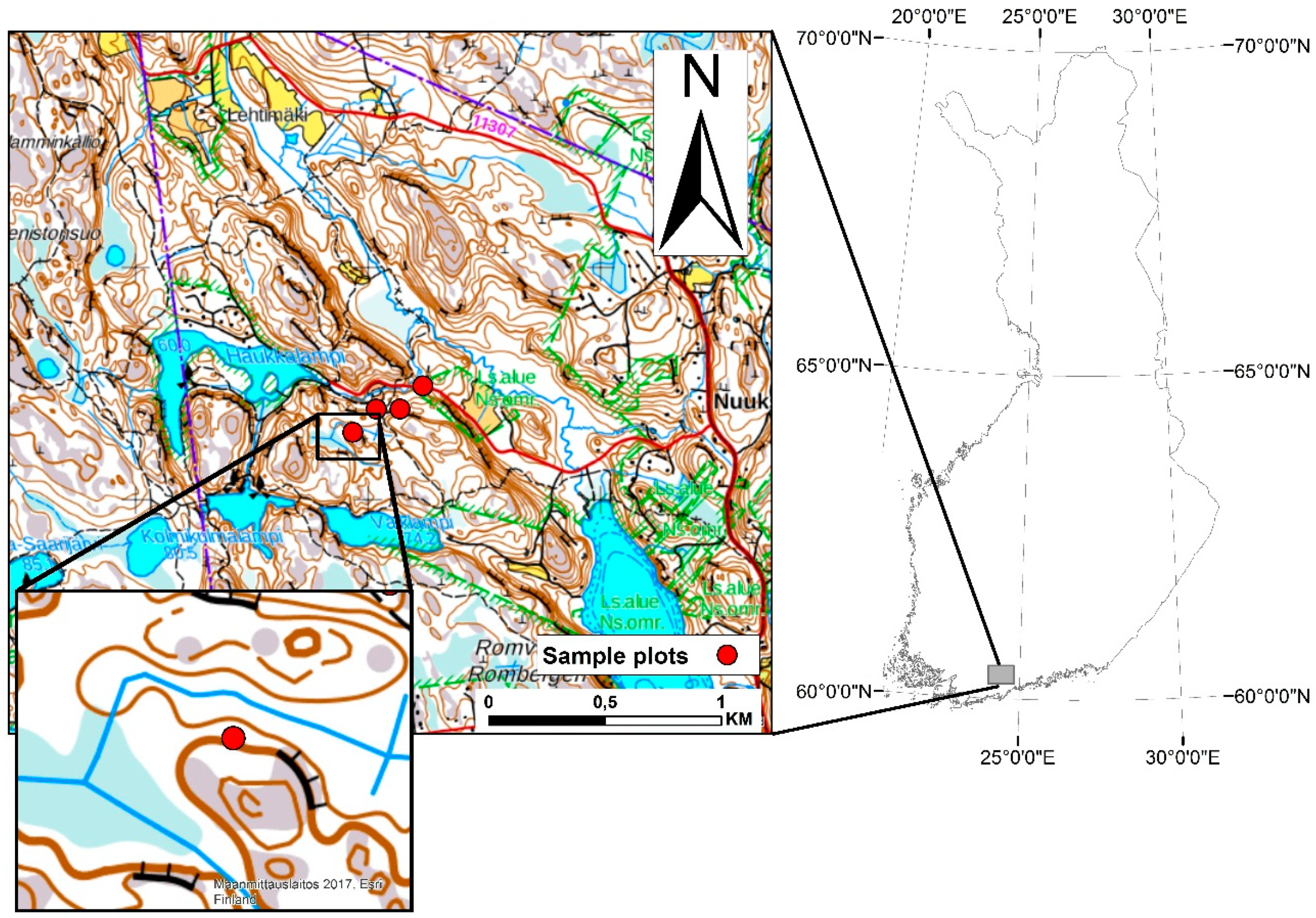
2.1. Study Area
2.2. Sample Plot Measurements
2.3. Data Processing and Measurement Method
2.4. Estimating Attributes for Individual Trees
2.5. Evaluating the Method’s Suitability for Detecting Change in Stem Volume and Stem Taper
3. Results
4. Discussion
5. Conclusions
Supplementary Materials
Author Contributions
Funding
Conflicts of Interest
References
- Husch, B.; Beers, T.W.; Kershaw, J.A. Forest Mensuration, 4th ed.; John Wiley & Sons: Hoboken, NJ, USA, 2003; p. 443. [Google Scholar]
- King, G.M.; Gugerli, F.; Fonti, P.; Frank, D.C. Tree growth response along an elevational gradient: Climate or genetics? Oecologia 2013, 173, 1587–1600. [Google Scholar] [CrossRef]
- Bradshaw, H.D., Jr.; Stettler, R.F.; Bradshaw, H.D. Molecular Genetics of Growth and Development in Populus. IV. Mapping Qtls with Large Effects on Growth, Form, and Phenology Traits in a Forest Tree. Genetics 1995, 139, 963–973. [Google Scholar]
- Alberto, F.J.; Aitken, S.N.; Alía, R.; González-Martínez, S.C.; Hänninen, H.; Kremer, A.; Lefèvre, F.; Lenormand, T.; Yeaman, S.; Whetten, R.; et al. Potential for evolutionary responses to climate change—Evidence from tree populations. Chang. Boil. 2013, 19, 1645–1661. [Google Scholar] [CrossRef]
- Mead, D.J.; Tamm, C.O. Growth and stem form changes in Picea abies as affected by stand nutrition. Scand. J. 1988, 3, 505–513. [Google Scholar] [CrossRef]
- Cherubini, P.; Fontana, G.; Rigling, D.; Dobbertin, M.; Brang, P.; Innes, J.L. Tree-life history prior to death: Two fungal root pathogens affect tree-ring growth differently. J. Ecol. 2002, 90, 839–850. [Google Scholar] [CrossRef]
- Dobbertin, M. Tree growth as indicator of tree vitality and of tree reaction to environmental stress: A review. Eur. J. 2005, 124, 319–333. [Google Scholar]
- Lyytikäinen-Saarenmaa, P.; Tomppo, E. Impact of sawfly defoliation on growth of Scots pine Pinus sylvestris (Pinaceae) and associated economic losses. Bull. Èntomol. Res. 2002, 92, 137–140. [Google Scholar] [CrossRef]
- Quine, C.P. Assessing the risk of wind damage to forests: Practice and pitfalls. In Wind and Trees; Coutts, M.P., Grace, J., Eds.; Cambridge University Press: Cambridge, UK, 1995; pp. 379–403. [Google Scholar]
- Solberg, S.; Andreassen, K.; Clarke, N.; Tørseth, K.; Tveito, O.E.; Strand, G.H.; Tomter, S. The possible influence of nitrogen and acid deposition on forest growth in Norway. Ecol. Manag. 2004, 192, 241–249. [Google Scholar] [CrossRef]
- Harper, J.L. Population Biology of Plants; The Blackburn Press: Caldwell, NJ, USA, 1977. [Google Scholar]
- Coomes, D.A.; Allen, R.B. Effects of size, competition and altitude on tree growth. J. Ecol. 2007, 95, 1084–1097. [Google Scholar] [CrossRef] [Green Version]
- Canham, C.D.; Lepage, P.T.; Coates, K.D. A neighborhood analysis of canopy tree competition: Effects of shading versus crowding. Can. J. 2004, 34, 778–787. [Google Scholar] [CrossRef]
- Aakala, T.; Berninger, F.; Starr, M. The roles of competition and climate in tree growth variation in northern boreal old-growth forests. J. Veg. Sci. 2018, 29, 1040–1051. [Google Scholar] [CrossRef]
- Avery, T.E.; Burkhart, H.E. Forest Measurements; Waveland Press: Long Grove, IL, USA, 2015. [Google Scholar]
- Repola, J. Biomass equations for birch in Finland. Silva Fenn. 2008, 42, 605–624. [Google Scholar] [CrossRef]
- Repola, J. Biomass equations for Scots pine and Norway spruce in Finland. Silva Fenn. 2009, 43, 625–647. [Google Scholar] [CrossRef]
- Laasasenaho, J. Taper Curve and Volume Functions for Pine, Spruce and Birch; The Finnish Forest Research Institute: Helsinki, Finland, 1982.
- Uusitalo, J. Pre-harvest measurement of pine stands for sawing production planning. Acta For. Fenn. 1997. [Google Scholar] [CrossRef]
- Kankare, V.; Vauhkonen, J.; Tanhuanpää, T.; Holopainen, M.; Vastaranta, M.; Joensuu, M.; Krooks, A.; Hyyppä, J.; Hyyppä, H.; Alho, P.; et al. Accuracy in estimation of timber assortments and stem distribution—A comparison of airborne and terrestrial laser scanning techniques. ISPRS J. Photogramm. Sens. 2014, 97, 89–97. [Google Scholar] [CrossRef]
- Lindner, M.; Maroschek, M.; Netherer, S.; Kremer, A.; Barbati, A.; Garcia-Gonzalo, J.; Seidl, R.; Delzon, S.; Corona, P.; Kolström, M.; et al. Climate change impacts, adaptive capacity, and vulnerability of European forest ecosystems. Ecol. Manag. 2010, 259, 698–709. [Google Scholar] [CrossRef]
- Seidl, R.; Rammer, W.; Spies, T.A. Disturbance legacies increase the resilience of forest ecosystem structure, composition, and functioning. Ecol. Appl. 2014, 24, 2063–2077. [Google Scholar] [CrossRef] [Green Version]
- Seidl, R.; Thom, D.; Kautz, M.; Martin-Benito, D.; Peltoniemi, M.; Vacchiano, G.; Wild, J.; Ascoli, D.; Petr, M.; Honkaniemi, J.; et al. Forest disturbances under climate change. Nat. Clim. Chang. 2017, 7, 395–402. [Google Scholar] [CrossRef] [Green Version]
- Zubizarreta-Gerendiain, A.; Pellikka, P.; Garcia-Gonzalo, J.; Ikonen, V.-P.; Peltola, H. Factors affecting wind and snow damage of individual trees in a small management unit in Finland. Silva Fennica 2012, 46, 181–196. [Google Scholar] [CrossRef]
- Liming, F.G. Homemade dendrometers. J. For. 1957, 55, 575–577. [Google Scholar]
- Daubenmire, R.F. An Improved Type of Precision Dendrometer. Ecology 1945, 26, 97–98. [Google Scholar] [CrossRef]
- Fritts, H.C.F.; Edwin, C. A New Dendrograph for Recording Radial Changes of a Tree. Forest Science 1955, 1, 271–276. [Google Scholar]
- Impens, I.I.; Schalck, J.M. A Very Sensitive Electric Dendrograph for Recording Radial Changes of a Tree. Ecology 1965, 46, 183–184. [Google Scholar] [CrossRef]
- Kinerson, R.S. A Transducer for Investigations of Diameter Growth. For. Sci. 1973, 19, 230–232. [Google Scholar]
- Phipps, R.L.; Gilbert, G.E. An electric dendrograph. Ecology 1960, 41, 389–390. [Google Scholar] [CrossRef]
- Reineke, L.H. A Precision Dendrometer. J. For. 1932, 30, 692–699. [Google Scholar]
- Liang, X.; Kankare, V.; Hyyppä, J.; Wang, Y.; Kukko, A.; Haggrén, H.; Yu, X.; Kaartinen, H.; Jaakkola, A.; Guan, F.; et al. Terrestrial laser scanning in forest inventories. ISPRS J. Photogramm. Sens. 2016, 115, 63–77. [Google Scholar] [CrossRef] [Green Version]
- Cabo, C.; Ordoñez, C.; López-Sánchez, C.A.; Armesto, J. Automatic dendrometry: Tree detection, tree height and diameter estimation using terrestrial laser scanning. Int. J. Appl. Earth Obs. Geoinformation 2018, 69, 164–174. [Google Scholar] [CrossRef]
- Henning, J.G.; Radtke, P.J. Detailed Stem Measurements of Standing Trees from Ground-Based Scanning Lidar. Forest Science 2006, 52, 67–80. [Google Scholar]
- Huang, H.; Li, Z.; Gong, P.; Cheng, X.; Clinton, N.; Cao, C.; Ni, W.; Wang, L. Automated Methods for Measuring DBH and Tree Heights with a Commercial Scanning Lidar. Photogramm. Eng. Sens. 2011, 77, 219–227. [Google Scholar] [CrossRef]
- Liang, X.; Hyyppa, J. Automatic Stem Mapping by Merging Several Terrestrial Laser Scans at the Feature and Decision Levels. Sensors 2013, 13, 1614–1634. [Google Scholar] [CrossRef] [PubMed] [Green Version]
- Maas, H.; Bienert, A.; Scheller, S.; Keane, E. Automatic forest inventory parameter determination from terrestrial laser scanner data. Int. J. Sens. 2008, 29, 1579–1593. [Google Scholar] [CrossRef]
- Koreň, M.; Mokroš, M.; Bucha, T. Accuracy of tree diameter estimation from terrestrial laser scanning by circle-fitting methods. Int. J. Appl. Earth Obs. Geoinformation 2017, 63, 122–128. [Google Scholar] [CrossRef]
- Pitkänen, T.P.; Raumonen, P.; Kangas, A. Measuring stem diameters with TLS in boreal forests by complementary fitting procedure. ISPRS J. Photogramm. Sens. 2019, 147, 294–306. [Google Scholar] [CrossRef]
- Saarinen, N.; Kankare, V.; Vastaranta, M.; Luoma, V.; Pyörälä, J.; Tanhuanpää, T.; Liang, X.; Kaartinen, H.; Kukko, A.; Jaakkola, A.; et al. Feasibility of Terrestrial laser scanning for collecting stem volume information from single trees. ISPRS J. Photogramm. Sens. 2017, 123, 140–158. [Google Scholar] [CrossRef]
- Ducey, M.J.; Granhus, A.; Ritter, T.; Von Lüpke, N.; Astrup, R. Approaches for estimating stand-level volume using terrestrial laser scanning in a single-scan mode. Can. J. 2014, 44, 666–676. [Google Scholar]
- Moskal, L.M.; Zheng, G. Retrieving forest inventory variables with terrestrial laser scanning (TLS) in urban heterogeneous forest. Remote Sens. 2012, 4, 1–20. [Google Scholar] [CrossRef]
- Pueschel, P.; Newnham, G.; Rock, G.; Udelhoven, T.; Werner, W.; Hill, J. The influence of scan mode and circle fitting on tree stem detection, stem diameter and volume extraction from terrestrial laser scans. ISPRS J. Photogramm. Sens. 2013, 77, 44–56. [Google Scholar] [CrossRef]
- Kankare, V.; Liang, X.; Yu, X.; Hyyppa, J.; Holopainen, M. Automated Stem Curve Measurement Using Terrestrial Laser Scanning. IEEE Trans. Geosci. Sens. 2014, 52, 1739–1748. [Google Scholar]
- Calders, K.; Newnham, G.; Burt, A.; Murphy, S.; Raumonen, P.; Herold, M.; Culvenor, D.; Avitabile, V.; Disney, M.; Armston, J. Nondestructive estimates of above-ground biomass using terrestrial laser scanning. Methods Ecol. Evol. 2015, 6, 198–208. [Google Scholar] [CrossRef]
- Yu, X.; Liang, X.; Hyyppä, J.; Kankare, V.; Vastaranta, M.; Holopainen, M. Stem biomass estimation based on stem reconstruction from terrestrial laser scanning point clouds. Sens. Lett. 2013, 4, 344–353. [Google Scholar] [CrossRef]
- Kankare, V.; Holopainen, M.; Vastaranta, M.; Puttonen, E.; Yu, X.; Hyyppä, J.; Vaaja, M.; Hyyppä, H.; Alho, P. Individual tree biomass estimation using terrestrial laser scanning. ISPRS J. Photogramm. Sens. 2013, 75, 64–75. [Google Scholar] [CrossRef]
- Holopainen, M.; Vastaranta, M.; Kankare, V.; Räty, M.; Vaaja, M.; Liang, X.; Yu, X.; Hyyppä, J.; Hyyppä, H.; Viitala, R. Biomass estimation of individual trees using stem and crown diameter TLS measurements. ISPRS Int. Arch. Photogramm. Remote Sens. Spat. Inf. Sci. 2011, 3812, 91–95. [Google Scholar] [CrossRef]
- Pfeifer, N.; Winterhalder, D. Modelling of tree cross sections from terrestrial laser scanning data with free-form curves. Int. Arch. of Photogramm. Remote Sens. Spat. Inf. Sci. 2004, 36, W2. [Google Scholar]
- Liang, X.; Hyyppä, J.; Kaartinen, H.; Lehtomäki, M.; Pyörälä, J.; Pfeifer, N.; Holopainen, M.; Brolly, G.; Francesco, P.; Hackenberg, J.; et al. International benchmarking of terrestrial laser scanning approaches for forest inventories. ISPRS J. Photogramm. Sens. 2018, 144, 137–179. [Google Scholar] [CrossRef]
- Sheppard, J.; Morhart, C.; Hackenberg, J.; Spiecker, H. Terrestrial laser scanning as a tool for assessing tree growth. iForest-Biogeosci. For. 2016, 10, 172. [Google Scholar] [CrossRef]
- Kaasalainen, S.; Krooks, A.; Liski, J.; Raumonen, P.; Kaartinen, H.; Kaasalainen, M.; Puttonen, E.; Anttila, K.; Mäkipää, R. Change Detection of Tree Biomass with Terrestrial Laser Scanning and Quantitative Structure Modelling. Remote. Sens. 2014, 6, 3906–3922. [Google Scholar] [CrossRef] [Green Version]
- Mengesha, T.; Hawkins, M.; Nieuwenhuis, M. Validation of terrestrial laser scanning data using conventional forest inventory methods. Eur. J. For. Res. 2015, 134, 211–222. [Google Scholar] [CrossRef]
- Srinivasan, S.; Popescu, S.C.; Eriksson, M.; Sheridan, R.D.; Ku, N.-W. Multi-temporal terrestrial laser scanning for modeling tree biomass change. Ecol. Manag. 2014, 318, 304–317. [Google Scholar] [CrossRef]
- Liang, X.; Hyyppa, J.; Kaartinen, H.; Holopainen, M.; Melkas, T. Detecting Changes in Forest Structure over Time with Bi-Temporal Terrestrial Laser Scanning Data. ISPRS Int. J. Geo-Inf. 2012, 1, 242–255. [Google Scholar] [CrossRef] [Green Version]
- Newnham, G.J.; Armston, J.D.; Calders, K.; Disney, M.I.; Lovell, J.L.; Schaaf, C.B.; Strahler, A.H.; Danson, F.M. Terrestrial Laser Scanning for Plot-Scale Forest Measurement. For. Rep. 2015, 1, 239–251. [Google Scholar] [CrossRef] [Green Version]
- Vastaranta, M.; Melkas, T.; Holopainen, M.; Kaartinen, H.; Hyyppä, J.; Hyyppä, H.J.P.J.F. Laser-based Field Measurements in Tree-Level Forest Data Acquisition. Photogramm. J. Finl 2009, 21, 51–61. [Google Scholar]
- Young-Pow, C.; Treitz, P.; Hopkinson, C.; Chasmer, L. Assessing forest metrics with a ground-based scanning lidar. Can. J. 2004, 34, 573–583. [Google Scholar]
- Luoma, V.; Saarinen, N.; Wulder, M.A.; White, J.C.; Vastaranta, M.; Holopainen, M.; Hyyppä, J. Assessing Precision in Conventional Field Measurements of Individual Tree Attributes. Forests 2017, 8, 38. [Google Scholar] [CrossRef]
- Schiffel, A. Form und Inhalt der Fichte (Form and volume of spruce). Mitt. aus d. forstl. Versuchsan. Osterreiche 1899, 24. [Google Scholar]
- Muller-Landau, H.C.; Condit, R.S.; Harms, K.E.; Marks, C.O.; Thomas, S.C.; Bunyavejchewin, S.; Chuyong, G.; Co, L.; Davies, S.; Foster, R.; et al. Comparing tropical forest tree size distributions with the predictions of metabolic ecology and equilibrium models. Ecol. Lett. 2006, 9, 589–602. [Google Scholar] [CrossRef] [Green Version]
- Dobbertin, M.; Neumann, M.; Schroeck, H.-W. Tree Growth Measurements in Long-Term Forest Monitoring in Europe. In Developments in Environmental Science; Elsevier BV: Amsterdam, The Netherlands, 2013; Volume 12, pp. 183–204. [Google Scholar]
- Tansey, K.; Selmes, N.; Anstee, A.; Tate, N.J.; Denniss, A. Estimating tree and stand variables in a Corsican Pine woodland from terrestrial laser scanner data. Int. J. Sens. 2009, 30, 5195–5209. [Google Scholar] [CrossRef]
- Seidel, D.; Hoffmann, N.; Ehbrecht, M.; Juchheim, J.; Ammer, C. How neighborhood affects tree diameter increment—New insights from terrestrial laser scanning and some methodical considerations. Ecol. Manag. 2015, 336, 119–128. [Google Scholar] [CrossRef]
- Wang, Y.; Lehtomäki, M.; Liang, X.; Pyörälä, J.; Kukko, A.; Jaakkola, A.; Liu, J.; Feng, Z.; Chen, R.; Hyyppä, J. Is field-measured tree height as reliable as believed—A comparison study of tree height estimates from field measurement, airborne laser scanning and terrestrial laser scanning in a boreal forest. ISPRS J. Photogramm. Sens. 2019, 147, 132–145. [Google Scholar] [CrossRef]


| Plot | Number of Trees, n | DBH, cm | h, m | ||||
|---|---|---|---|---|---|---|---|
| Mean | Min | Max | Mean | Min | Max | ||
| 1 | 10 | 10.5 | 7.6 | 14.5 | 10.2 | 7.1 | 12.8 |
| 2 | 6 | 30.7 | 26.8 | 39.0 | 26.9 | 24.7 | 29.7 |
| 3 | 9 | 22.1 | 7.2 | 45.0 | 19.4 | 5.6 | 31.0 |
| 4 | 10 | 31.2 | 6.2 | 50.7 | 25.4 | 5.0 | 34.0 |
| Total | 35 | 22.8 | 6.2 | 50.7 | 19.8 | 5.0 | 34.0 |
| TAP | f | q0.5 | HDR | |
|---|---|---|---|---|
| p-value | 0.0023 | 0.0589 | 0.0081 | 0.7606 |
| ΔVol, m3 | ΔTAP, cm | Δf | Δq0.5 | ΔHDR | |
|---|---|---|---|---|---|
| Mean | 0.226 | −0.8 | 0.03 | 0.07 | 0.01 |
| Std.dev | 0.298 | 1.5 | 0.09 | 0.14 | 0.10 |
| Mean relative change | 65.0% | −13% | 9% | 15% | 1% |
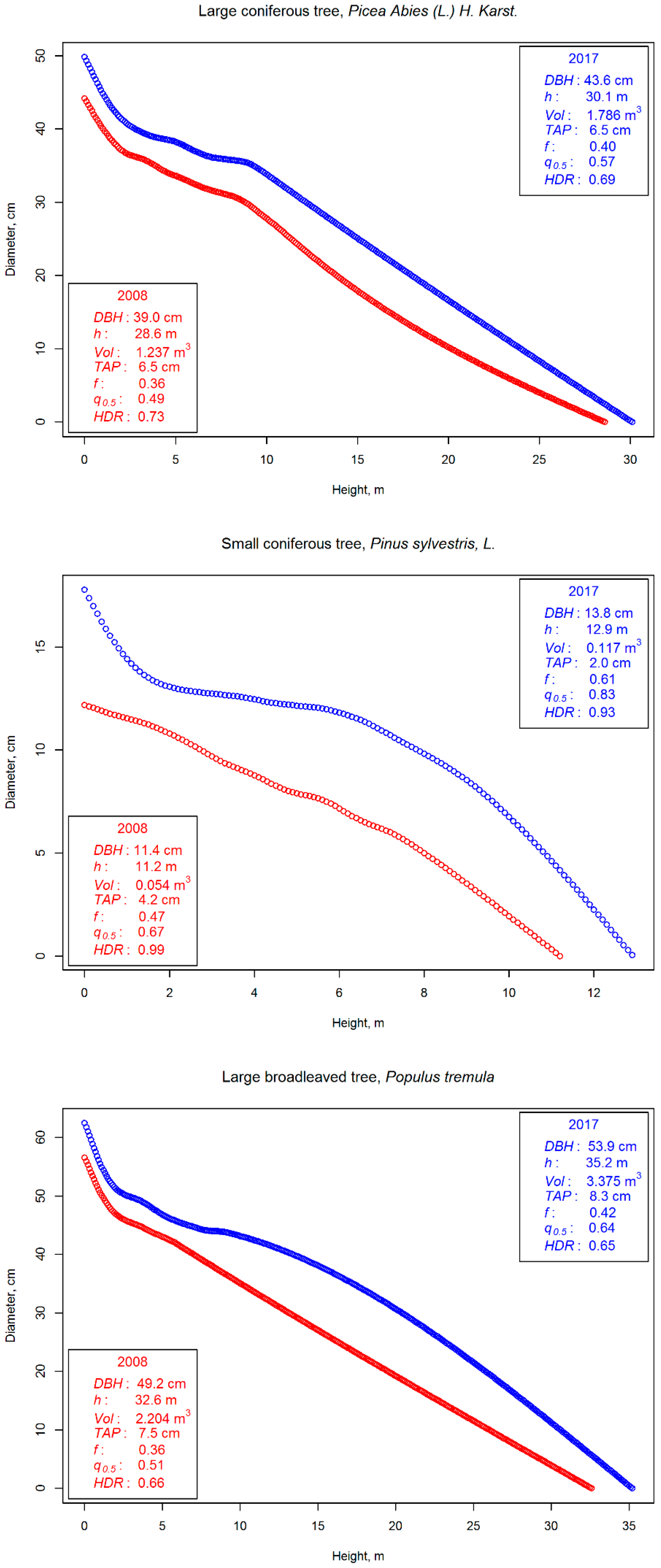
| Species Class | Mean DBH (cm) 2008 | Mean h (m) 2008 | Mean Vol (m3) 2008 | ΔVol (%) | ΔTAP (%) | Δf (%) | Δq0.5 (%) | ΔHDR (%) |
|---|---|---|---|---|---|---|---|---|
| Pinus sylvestris, L. | 10.5 | 10.2 | 0.049 | 125% | −34% | 9% | 13% | 6% |
| Picea Abies (L.) H. Karst | 27.3 | 23.8 | 0.796 | 44% | −12% | 9% | 15% | −2% |
| Betula pendula | 34.0 | 28.5 | 1.070 | 21% | 9% | 18% | 35% | −1% |
| Other broadleaved | 23.8 | 19.1 | 0.735 | 52% | 3% | 1% | 4% | 1% |
© 2019 by the authors. Licensee MDPI, Basel, Switzerland. This article is an open access article distributed under the terms and conditions of the Creative Commons Attribution (CC BY) license (http://creativecommons.org/licenses/by/4.0/).
Share and Cite
Luoma, V.; Saarinen, N.; Kankare, V.; Tanhuanpää, T.; Kaartinen, H.; Kukko, A.; Holopainen, M.; Hyyppä, J.; Vastaranta, M. Examining Changes in Stem Taper and Volume Growth with Two-Date 3D Point Clouds. Forests 2019, 10, 382. https://doi.org/10.3390/f10050382
Luoma V, Saarinen N, Kankare V, Tanhuanpää T, Kaartinen H, Kukko A, Holopainen M, Hyyppä J, Vastaranta M. Examining Changes in Stem Taper and Volume Growth with Two-Date 3D Point Clouds. Forests. 2019; 10(5):382. https://doi.org/10.3390/f10050382
Chicago/Turabian StyleLuoma, Ville, Ninni Saarinen, Ville Kankare, Topi Tanhuanpää, Harri Kaartinen, Antero Kukko, Markus Holopainen, Juha Hyyppä, and Mikko Vastaranta. 2019. "Examining Changes in Stem Taper and Volume Growth with Two-Date 3D Point Clouds" Forests 10, no. 5: 382. https://doi.org/10.3390/f10050382