Article

Linking Terrestrial LiDAR Scanner and Conventional Forest Structure Measurements with Multi-Modal Satellite Data

1
Laboratory of Geo-Information Science and Remote Sensing, Wageningen University, Droevendaalsesteeg 3, 6708 PB Wageningen, The Netherlands
2
Forest Ecology and Forest Management Group, Wageningen University and Research Centre, P.O. Box 47, NL-6700 AA Wageningen, The Netherlands
3
GOFC-GOLD Land Cover Project Office, Droevendaalsesteeg 3, 6708 PB Wageningen, The Netherlands
*
Author to whom correspondence should be addressed.
Forests 2019, 10(3), 291; https://doi.org/10.3390/f10030291
Submission received: 25 January 2019 / Revised: 19 March 2019 / Accepted: 22 March 2019 / Published: 26 March 2019

Abstract

:
Obtaining information on vertical forest structure requires detailed data acquisition and analysis which is often performed at a plot level. With the growing availability of multi-modal satellite remote sensing (SRS) datasets, their usability towards forest structure estimation is increasing. We assessed the relationship of PlanetScope-, Sentinel-2-, and Landsat-7-derived vegetation indices (VIs), as well as ALOS-2 PALSAR-2- and Sentinel-1-derived backscatter intensities with a terrestrial laser scanner (TLS) and conventionally measured forest structure parameters acquired from 25 field plots in a tropical montane cloud forest in Kafa, Ethiopia. Results showed that canopy gap-related forest structure parameters had their highest correlation (|r| = 0.4 − 0.48) with optical sensor-derived VIs, while vegetation volume-related parameters were mainly correlated with red-edge- and short-wave infrared band-derived VIs (i.e., inverted red-edge chlorophyll index (IRECI), normalized difference moisture index), and synthetic aperture radar (SAR) backscatters (|r| = −0.57 − 0.49). Using stepwise multi-linear regression with the Akaike information criterion as evaluation parameter, we found that the fusion of different SRS-derived variables can improve the estimation of field-measured structural parameters. The combination of Sentinel-2 VIs and SAR backscatters was dominant in most of the predictive models, while IRECI was found to be the most common predictor for field-measured variables. The statistically significant regression models were able to estimate cumulative plant area volume density with an R2 of 0.58 and with the lowest relative root mean square error (RRMSE) value (0.23). Mean gap and number of gaps were also significantly estimated, but with higher RRMSE (R2 = 0.52, RRMSE = 1.4, R2 = 0.68, and RRMSE = 0.58, respectively). The models showed poor performance in predicting tree density and number of tree species (R2 = 0.28, RRMSE = 0.41, and R2 = 0.21, RRMSE = 0.39, respectively). This exploratory study demonstrated that SRS variables are sensitive to retrieve structural differences of tropical forests and have the potential to be used to upscale biodiversity relevant field-based forest structure estimates.

1. Introduction

The horizontal and vertical structure of vegetation is important as it provides niches for forest-dependent plant and animal species [1]. The structural complication of habitats has direct effect on the availability of resources and microclimate conditions which can affect for example the abundance and diversity of species. Even though tropical forests host the most endemic and valuable biodiversity, they are threatened with increasing deforestation and forest degradation that alters the complexity of the habitat [2]. Understanding the structural configuration and diversity of tropical forest habitats will help explain the state of forest degradation and the resulting biodiversity dynamics. Thus, forest habitat heterogeneity has become one of the most commonly used indicators in forest biodiversity conservation and management studies [3,4]. Ecosystem structure (encompassing the vertical structural complexity and the horizontal fragmentation status of habitats) is listed by The Group on Earth Observations Biodiversity Observation Network (GEOBON) as one of the essential biodiversity variables (EBVs) to monitor and to understand global biodiversity change [5], contributing towards the realization of the United Nations (UN) Convention on Biological Diversity (CBD) Aichi targets [6]. However, the accurate characterization and monitoring of forest structure is challenging. This is often due to the complex three-dimensional configuration of tropical forests [7].
Ground-based traditional measurements are among the most accurate methods for forest structure estimations and are a typical source for conservation studies [8,9]. However, their time-consuming, spatially limited, and laborious nature opened up a growing exploration towards using remotely sensed datasets to overcome such limitations [10,11]. In this context, light detection and ranging (LiDAR) is a rather recent remote sensing technique that is increasingly being used in forestry. It has active sensors that transmit laser pulses to targets and uses the time-of-flight principle to measure the distance to an object. The three-dimensional position of an object can be defined using the known position of the sensor and the range measurement between the sensor and the targeted object [12]. Information on the three-dimensionality of forests helps with the understanding of essential habitat parameters such as gap formation and dynamics, light penetration, and understory vegetation [13]. Terrestrial laser scanner (TLS) measurements are used for rapid and detailed quantification of forest structure variables such as tree height [14,15], vertical plant profiles [16], canopy gap fraction [17], and diameter at breast height (DBH) measurements [18,19]. These measurements are made at a plot scale and can be used to characterize forest structural complexity across different forest types [20]. Even though TLS data provide good estimates of forest structure, the small coverage, operational costs, and complex analytical process limit its usability [15].
Concomitantly, satellite remote sensing (SRS) is being explored as an alternative resource to facilitate synoptic and scalable forest structure estimation [21,22]. The use of SRS for structural assessment of forest environments is based on the distinct characteristics expected from forest canopies when in contact with solar radiation and/or with signals from active satellites. Even though three-dimensional forest structure elements such as tree height and number of layers are not yet directly extractable from the commonly used optical satellite images, the spectral signals recorded from leaf reflectance across different spectral regions could be used to assess biophysical parameters of forests [23]. Especially, the leaf reflectance in the red-edge, near-infrared (NIR), and middle infrared regions are affected by chlorophyll content, leaf structure, and water content, respectively. Therefore, short wave infrared (SWIR), NIR, red-edge bands are often used to calculate vegetation indices that could represent the amount and/or condition of vegetation within a pixel [24]. Several studies have demonstrated the usability and relation of spectral vegetation indices (VIs) with field-measured vertical forest structure attributes such as tree species diversity [22], biomass [23,25], and tree height [26]. Here, the spatial, spectral, radiometric, and temporal resolution of images affects the usability of SRS for extracting structural information of forests. Medium-spatial resolution imagery such as Landsat images are the most commonly used data for studying time series dynamics of biophysical forest attributes [26,27,28]. The inclusion of red-edge spectrum-specific bands, and the availability of higher spatial resolution images in Sentinel-2 have improved the use of SRS data to assess forest structure-related parameters [29,30].
Continuous acquisition of cloud and haze free optical images, especially over the tropics, is difficult. Synthetic aperture radar (SAR) acquires continuous imagery that is largely independent of cloud cover and solar illumination condition. SAR sensors transmit polarized microwaves (on a horizontal (H) or vertical (V) plane) that interact with surface objects, and record the backscattered signal (in either a horizontal (H) or vertical (V) plane). In the case of forests, complex structural components (trunks, branches, and leaves) lead to typical volume scattering which can be identified well in the HV (horizontal transmit and vertical received) polarization [31]. The wavelength, incidence angles, and polarizations of SAR signals, as well as the canopy complexity of forests, determines backscatter intensities. Long wavelengths (i.e., L- and P-band) have a greater ability to penetrate the canopy and acquire backscatter signals from stems and large branches [32]. For example, with ALOS-2 PALSAR-2 L-band, high-HV backscatters are expected from dense vegetation of tropical forests, which correlates with biomass [33]. The short wavelengths (i.e., X-, C-, S-band) are mainly scattered back from the upper tree crown and less from beneath; thus, mainly indicating on canopy structural variables [34]. In addition to structural components, other environmental factors such as topography and moisture causes variations in backscatter signals [35,36].
The ecological application of SRS is supported by the growing availability of very high-spatial resolution satellite data (e.g., RapidEye, IKONOS, and PlanetScope), and with the freely available high- to medium-spatial resolution data from Sentinel and Landsat satellites. The unique characteristics of each SRS data type can provide valuable input in acquiring timely and continuous information on forest structure and to the understanding of its implication on habitat requirements of forest-dependent species [37]. Coupled with powerful analytical approaches, SRS datasets could provide wall-to-wall and repeatable information on forest structure which would otherwise be very expensive to collect with field-based analysis.
The overall objective of this study was to explore, at plot level, the applicability of optical SRS (i.e., PlanetScope, Sentinel-2, Landsat-7); and SAR images (ALOS-2 PALSAR-2 and Sentinel-1), for estimating field-measured (i.e., using TLS and conventional forestry measurements) forest structure parameters in the tropical cloud forests of Kafa, Ethiopia. In doing so, we aim (i) to identify the relationship between SRS-derived variables and field-measured forest structure parameters; and (ii) to develop models estimating field-measured forest structure parameters through the fusion of SRS-derived predictors. We hypothesize that SRS-derived indices and backscatters will show a significant correlation with some TLS measurements; and that SRS variable-based models will be able, to some extent, to estimate the forest structure of montane cloud forest.

2. Materials and Methods
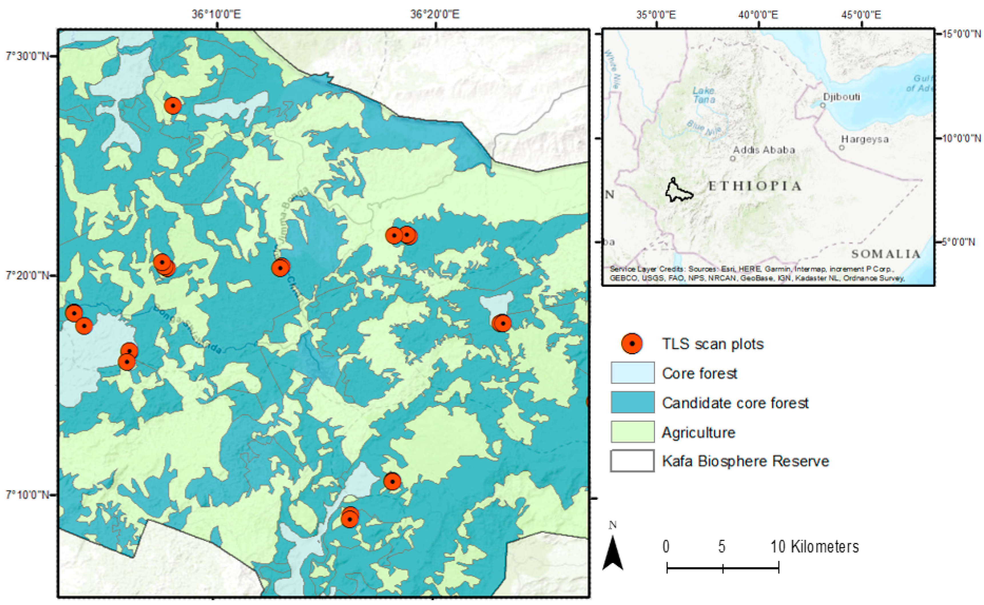
2.1. Study Site

The study area is located in Kafa biosphere reserve (KBR), Ethiopia (36°3′22.51″ E, 7°22′13.67″ N) (Figure 1). It covers a total area of 744,919 ha, of which 47% is comprised of different forest types (i.e., intact to highly degraded) and diverse habitats (i.e., Sub-Afroalpine to wetland). The Afromontane mountain cloud forests of KBR are the origin of wild varieties of Coffea Arabica L., and home to many endemic and threatened species [38]. However, the ongoing deforestation, forest fragmentation, and forest degradation due to anthropogenic pressure raise threats on the biological diversity of KBR [39], thus placing it as part of the Eastern Afromontane Biodiversity Hotspot and under the national forest priority area protection schemes [38].

2.2. Field Data Collection

The field data on forest structure were collected in November 2015 in Kafa biosphere reserve, Ethiopia, consisting of 25 plots across four forest management types (Intact: 7 plots, coffee forest: 8 plots, silvopasture: 7 plots, and plantation: 3 plots). The details on the collection and analysis of the TLS and conventional forest measurements can be found in Decuyper et al. [20]. In short, a stratified sampling design was made based on various GIS data layers (i.e., fragmentation map, land use/cover map, and biodiversity assessment plots) of the study area to select field plots for measurements. The chosen plot locations were representative of their surrounding forest type. TLS measurements were made with a RIEGL VZ-400 terrestrial laser scanner (RIEGL Laser Measurement Systems GmbH, Horn, Austria). From the 25 plots, 21 plots had a radius of 20 m, while 4 plots had a 10 m radius due to difficult terrain. Five scanning positions (i.e., one in the center and four in the cardinal directions) were used per each plot to acquire three-dimensional measurements.
The point cloud data was preprocessed and co-registered using RiSCAN PRO software (RIEGL Horn, Austria). The vertical profiles of Plant Area Volume Density (PAVD) were derived based on a method developed by Calders et al. [40], while the canopy gap and canopy height parameters, were derived by analyzing the point clouds in CompuTree point cloud analysis open source software [41]. The PAVD from 0 m to 10 m were considered as understory vegetation, while PAVD from 0 m to top of canopy level were considered as cumulative PAVD [40]. Additional canopy parameters (i.e., canopy heights, canopy gaps, and canopy openness) were derived from digital height models produced at a 0.5m resolution. The canopy gaps derived from TLS were defined by canopy height of <10 m and with an area of ≥1 m2 [20].
Conventional forestry measurements were also taken on all 25 plots. Measurements included diameter at breast height (DBH), total basal area (BA), tree density, and tree species identification. Above-ground biomass (AGB) was derived by using the wood density values for African tropical moist forests [42]. The field-measured structural variables (Table 1) showed distinct characteristics across different forest management types.

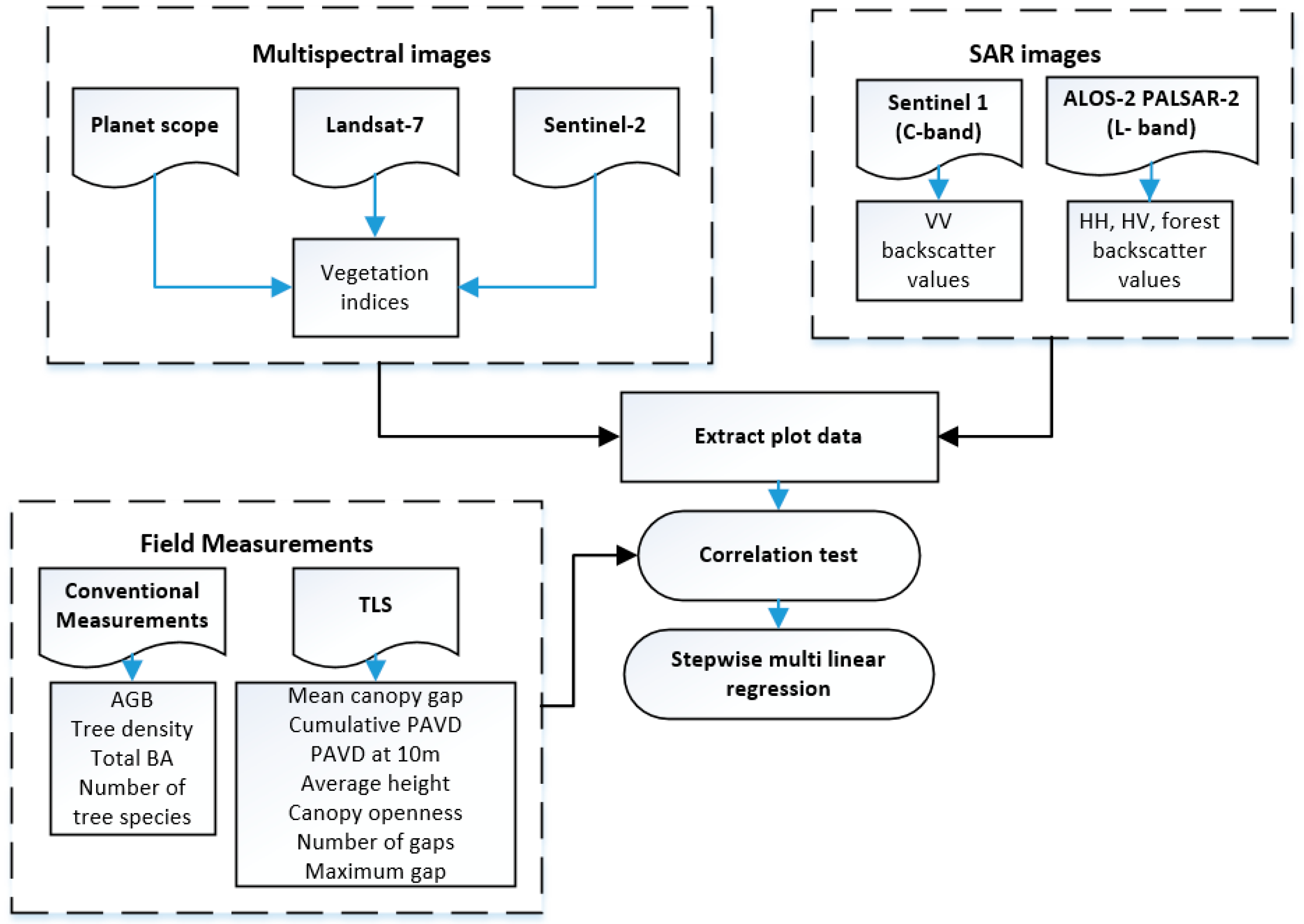
2.3. Satellite Remote Sensing Data

An overview of the datasets used in this study is presented in Table 2. We acquired the least clouded scenes from PlanetScope, Sentinel-2, Landsat-7, Sentinel-1, and ALOS-2 PALSAR-2 satellites that are closest to the field campaign date (i.e., November 2015). Since the change in forest vertical structure is often a slow process, we do not assume the time-lag between field data collection and SRS data acquisition will affect the relations between field parameters and SRS-derived variables. The very high-spatial resolution PlanetScope images were accessed through the PlanetScope ambassadorship quota (https://www.planet.com/markets/education-and-research/). The four-band analytic PlanetScope (red, green, blue, and near infra-red) images were downloaded as orthorectified top of atmosphere (TOA) radiance products (Level 3B). The images were converted to TOA reflectance using the PlanetScope guide [43]. The Sentinel-2 Multispectral Imager Instrument (MSI) Level 1-C images were acquired from the Sentinel Scientific Data Hub [44]. The products were atmospherically corrected using Sen2Cor [45]. The geometrically and atmospherically corrected Landsat-7/ETM+ images were obtained from The United State of America’s Geological Survey (USGS) Landsat surface Reflectance (SR) archive (http://landsat.usgs.gov/CDR_LSR.php). The CFmask cloud-shadow mask product [46] was used to generate cloud- and cloud shadow-free images.
The SAR images from Sentinel-1 and ALOS-2 PALSAR-2 were obtained for three time steps, covering the wet and dry season. The Sentinel-1 VV-polarized C-band SAR images were acquired in interferometric wide swath mode (IWS, 250 km swath width) and downloaded from the Sentinel science hub (https://scihub.copernicus.eu/). The ALOS-2 PALSAR-2 HV-polarized L-band SAR images were acquired in fine-beam dual mode (FBD, 70 km swath width) and obtained from the ALOS-2 data archive (https://auig2.jaxa.jp/ips/home). The pre-processing and speckle removal of the SAR images was conducted following the procedure by Reiche et al. [47]. Both Sentinel-1 and ALOS-2 PALSAR-2 backscatter images were geocoded to 30 m resolution and were co-registered to Landsat images [47].

Satellite Remote Sensing-Derived Vegetation Indices and Backscatter Intensities

The red (R), green (G), and near infrared (NIR) bands of optical SRS images, with their original spatial resolution (Table 2), were used to calculate forest biophysical sensitive VIs [22,23,48,49,50] for each field plot and their surrounding forests in the KBR (Table 3). The indices produced were green normalized difference vegetation index (GNDVI), enhanced vegetation index (EVI), and green chlorophyll index (CI green). In addition, the shortwave infrared (SWIR) bands of Sentinel-2 and Landsat-7 were used to produce the normalized difference moisture index (NDMI), while the Sentinel-2 specific red-edge bands were used to produce inverted red-edge chlorophyll Index (IRECI).
The C-band VV-polarization from Sentinel-1, as well as the L-band HH and HV polarizations from ALOS-2 PALSAR-2, were used to acquire backscatter intensities [35,56] and to calculate forest-specific backscatter (FB) values [56]. Vegetation indices were calculated for a 3 m × 3 m raster of pixels of Planetscope, for 10 m × 10 m raster pixels of Sentinel-2 10 m bands, as well as for 20 m × 20 m raster pixels of Sentinel-2 red-edge bands. Similarly, 30 m × 30 m raster pixels were used to calculate vegetation indices for Landsat-7 images, and for calculating backscatter values of Sentinel-1 and ALOS PALSAR-2 images. For the high-spatial resolution-derived SRS variables, the area-weighted mean values of the variables were calculated by overlaying the circular ground plots of 20 m radius (area = 0.1 ha). Whereas for the medium-spatial resolution images, we extracted the area-weighted mean values with an overlay of 50 m radius plots. We chose to use the 50 m radius of plots for the medium resolution images as our field plots are representative of the surrounding forest area, and especially for the SAR images, looking into multiple pixels will help eliminate errors and noises while using small raster pixels [35,58]. In addition, to account for the limited sensitivity of SAR backscatters to forest structure during wet seasons due to vegetation and soil moisture [33,59], we calculated the temporal standard deviation (TSD) of backscattered values between the three SAR images (Table 2).

2.4. Statistical Methods

The study initially assessed the relationship between field-measured forest structure parameters and SRS-derived variables based on the Pearson correlation coefficient using ‘Hmisc’ package [60] with the RStudio software [61]. We used p < 0.05 as the threshold to identify significant correlations. Then, the field-measured forest parameters were modeled as a function of their correlated SRS variables (Figure 2). Multiple linear regression models with both forward and backward stepwise selection procedure were developed to combine and assess the contribution of SRS variables in predicting field-measured structural parameters. The SRS variables used in the multiple linear regression models were derived using the original pixel size of the high- to medium-spatial resolution images (Table 2), so as to capture the possible detailed information on the corresponding field-measured structural variables from the high-resolution SRS images. Multicollinearity between predictors was checked to avoid overfitting. Predictors with correlations of >0.6 were excluded and a variance inflation factor of <2 was set as a threshold. The multiple linear regression model is described as:
FMP = β0 + β1x1 + β2x2 +…+ βpxp + ε
where FMP is the response field-measured parameter, x1, x2, …, xp, are SRS variables, β represents model coefficients, and ε is the additive normal distributed error term with zero mean.
The stepwise model selection procedure identified the best-fitted model based on Akaike’s information criterion (AIC). The accuracy of the fitted models was evaluated by exploring the coefficient of determination (R2), and the root mean square error (RMSE) between observed and predicted forest structural parameters. Relative root mean square error (RRMSE) is used to make the RMSE’s of the estimation models comparable. We tested the distribution of our dataset and used a logarithmic transformation on field-measured parameters that did not have a normal distribution (i.e., mean gap, PAVD at 10 m, maximum gap, AGB, and total basal area). The predicted results were then back-transformed and compared with the observed structural parameters.

3. Results

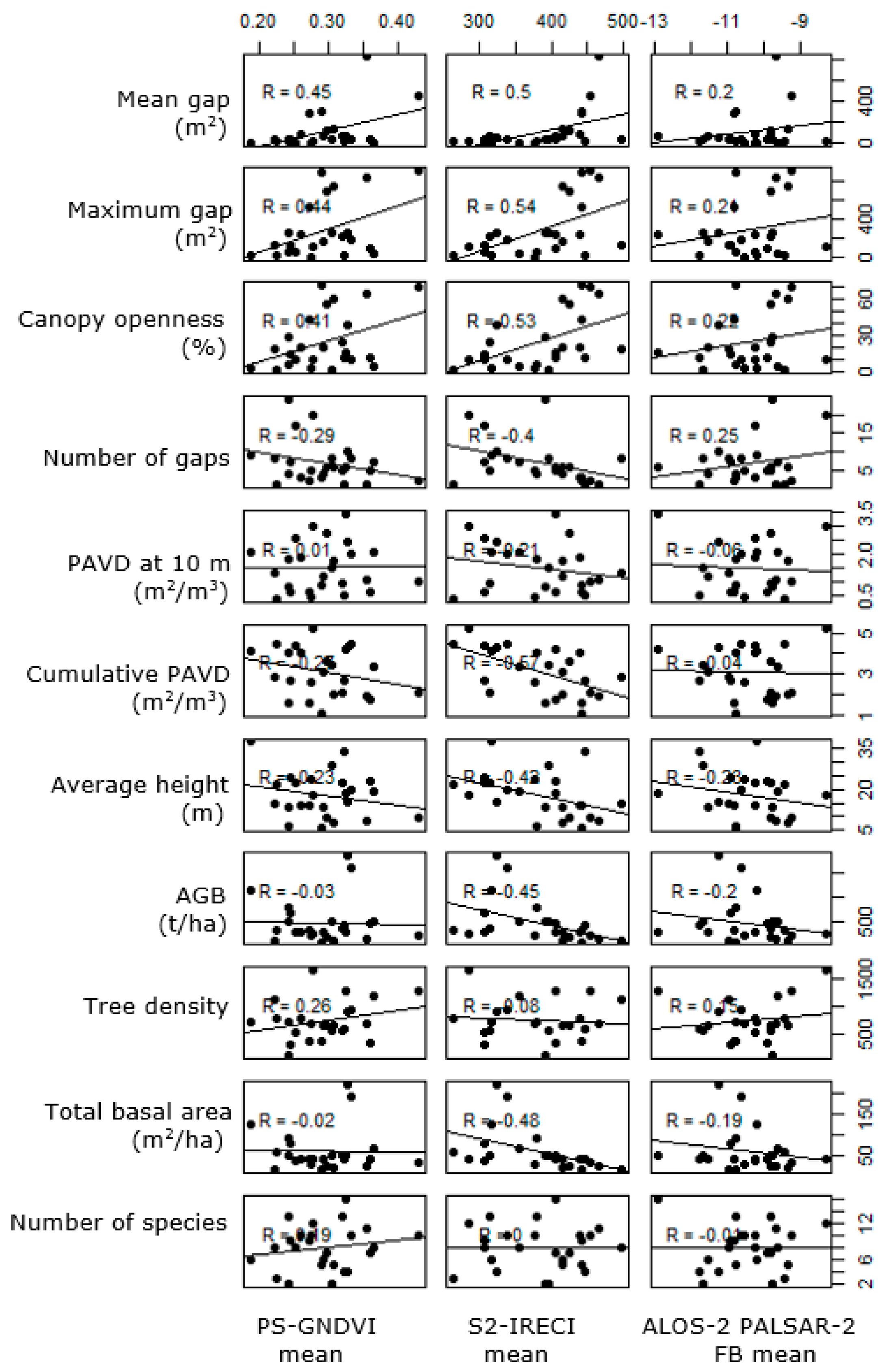
3.1. Correlation Analysis

The relationship between field-measured structural parameters and satellite remote sensing-derived variables based on the visualization of scatter plots showed most relationships were linear, especially with the optical VIs. Figure 3 represents a scatter plot of the relationship between the field-measured structural parameters and the most correlated SRS variables from optical and SAR domain. The Pearson correlation coefficient showed the strength and significance of these relationships. We found statistically significant correlations between the field-measured structural parameters and the SRS-derived variables (Table 4).
In summary, the gap-related parameters (i.e., mean gap, maximum gap, and canopy openness) especially showed highly significant correlations (|r| = 0.4 − 0.48, p < 0.01) with PlanetScope-derived GNDVI and CIGreen, as well as with Sentinel 2-derived EVI and IRECI VIs (|r| = 0.5 − 0.75, p < 0.01), as well as with Sentinel-1 VV TSD (|r| = 0.4 − 0.43, p < 0.05). The PAVD parameters, on the other hand, showed significant correlations (|r| = −0.57 to 0.49, p < 0.01) with the Sentinel-2 (IRECI), Landsat-7 (CIGreen, NDMI), as well as with Sentinel-1, and ALOS-2 PALSAR-2 (HV TSD) SAR backscatter variables. In addition, the conventionally measured structural parameters (except number of tree species) were found to be highly correlated (|r| = −0.45 to 0.43, p < 0.05) with Sentinel-2-derived NDMI and IRECI indices as well as with Landsat-7-derived GNDVI and CIGreen indices (|r| = 0.41 − 0.44, p < 0.05). No significant correlations were found between the number of species and SRS variables.

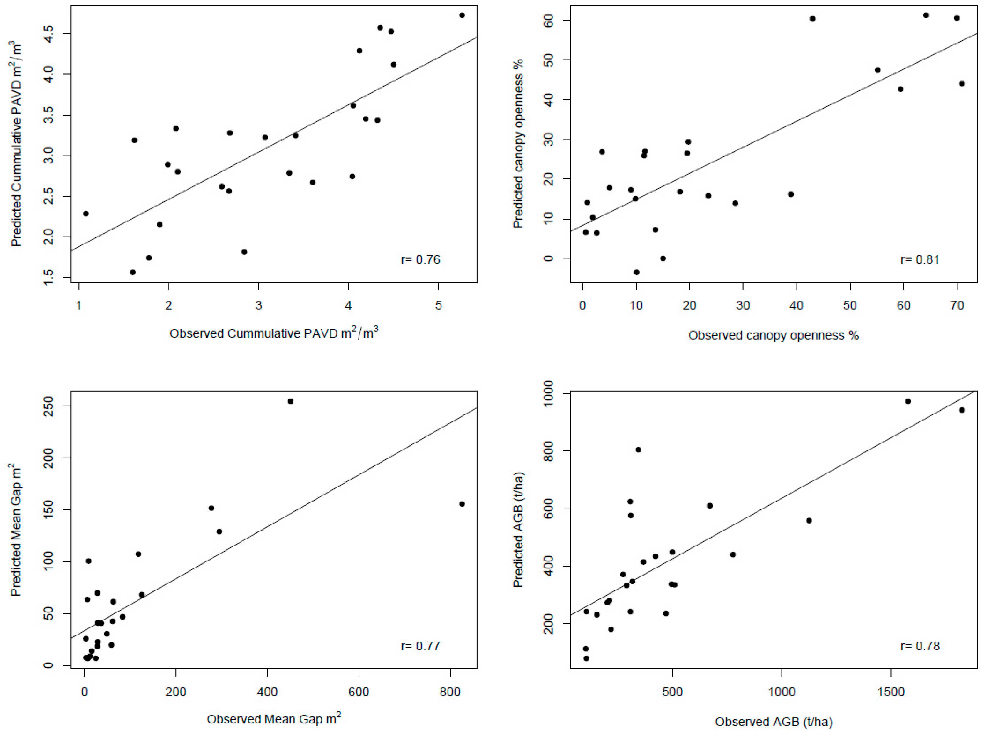
3.2. Prediction of Field-Measured Forest Structure Parameters

Stepwise multi-linear regression was used for identifying best-fitted models to predict field-observed forest structure parameters. The model with the lowest AIC was chosen as the best one and was used to make predictions. All field-measured structural parameters were estimated by the fusion of several SRS-derived variables, showing the complementarity of SRS products (Table 5). Field-measured variables that were log-transformed (i.e., mean gap, PAVD at 10 m, maximum gap, AGB, and total basal area) were able to be estimated using SAR data. Sentinel-2-based variables were dominant in most of the predictive models. IRECI was the common predictor for most field-measured variables, and especially in estimating mean gap, AGB, and cumulative PAVD. Backscatter values from ALOS-2 PALSAR-2 and Sentinel-1 were also valid predictors in most models, especially for predicting PAVD at 10 m and the number of gaps. Indices from PlanetScope and Landsat-7 were found to be the least relevant on the predictive models. The combination of red-edge band-derived IRECI of Sentinel-2, and ALOS-2 PALSAR-2 backscatters were found very important for AGB, total BA, and canopy openness estimation.
All regression models (except for average height) were statistically significant (p < 0.01), with cumulative PAVD having the highest R2 (0.58) and lowest RRMSE value (0.23) (Table 5). For TLS-measured structural parameters, number of gaps and mean gap were well predicted (R2 = 0.68, RRMSE = 0.58, and R2 = 0.66, RRMSE = 0.54, respectively), while PAVD at 10 m and average height had poor predictions (R2 = 0.47, RRMSE = 0.41, and R2 = 0.37, RRMSE = 0.35, respectively). As for the conventional measurements, S2-IRECI and S2-NDMI explained much of the variation in AGB and total basal area (R2 = 0.62, RRMSE = 0.61, and R2 = 0.61, RRMSE = 0.55, respectively), while tree density and number of species had the lowest R2 values (R2 = 0.28, RRMSE = 0.41, and R2 = 0.21, RRMSE = 0.39, respectively). The relationship between field-measured (observed) (e.g., cumulative PAVD, canopy openness, mean gap, and AGB) and satellite remote sensing-predicted forest structure variables are visualized in Figure 4.

4. Discussion

The study shows that optical SRS-derived VIs, despite being underestimated for saturating in forest environments, can inform on forest structural differences. Indices calculated with higher weighing coefficients of the SWIR, NIR, and red-edge bands were sensitive to most field-measured forest structure parameters (Table 4). The sensitivity of SWIR to plant leaf water content, which is correlated with canopy biomass, enabled NDMI to respond to vegetation volume-related parameters, thus supporting the estimation of the TLS-measured cumulative PAVD, and the conventionally measured AGB and basal area (Table 5), as did the sensitivity of NIR to multiple scattering of canopy leaves, canopy gaps, and shadowing; thus, sensitivity to forest canopy structure was associated with EVI’s response towards the estimation of TLS-measured, canopy gap-related parameters (Table 5). The canopy chlorophyll content and leaf area index (LAI) sensitive red-edge bands of Sentinel-2 [55], were associated with both vegetation volume [62] and canopy gaps [63], which made S2-IRECI the most important index in estimating both conventionally and TLS-measured structural parameters (Table 5). Our findings are in line with the studies of Huete et al. [64], Healey et al. [65], Brede et al. [66], and Martin et al. [67], that also found the SWIR, NIR, and red-edge bands important in exploring forests’ biophysical parameters. The PlanetScope-derived vegetation indices, despite being correlated with many canopy gap-related parameters, did not have a significant contribution to the prediction of field-measured structural estimates. This stands in contrast to other studies that found highly significant relationships between vegetation indices derived from very high-resolution images and forest structure parameters. Meng et al. [22] and Wallner et al. [50], for example, successfully estimated basal area, DBH, and other diversity indices using spectral and textural information from SPOT-5 and RapidEye images, respectively. Similar to the findings of this study, Baloloy et al. [23] found Sentinel-2- and RapidEye-based predictors to perform better towards estimating AGB compared to PlanetScope-derived predictors. A study by Houborg et al. [68] suggests that the potential applicability of PlanetScope-derived variables for monitoring might be limited due to its low radiometric quality and cross-sensor inconsistencies. The topographical and structural complexity of tropical forests can also affect estimation qualities. Castillo-Santiago et al. [42] stated that the nature of tropical forests and the quantity of shadows present on satellite images affects the prediction of forest structure variables using vegetation indices. Such topographic factors could also affect our study plots as they are located in cloud forest characterized by rough terrain and a mixture of different forest types (i.e., intact forest to silvopasture). Due to the terrain conditions, our plot sizes are small, which could complicate the exact link between SRS and field-measured parameters. In addition, the conservative threshold we used to identify canopy gaps (canopy height of <10 m and with an area of ≥1 m2) from the TLS measurements, and the reflectance of the dense understory in such forests despite having gaps, could have also affected the sensitivity of vegetation indices to the mean and maximum canopy gap parameters.
As for the SAR data, the standard deviation of multi-temporal ALOS-2 PALSAR-2 backscatters (HV-TSD), and forest backscatter (FB-TSD) were significant predictors of field-measured structural parameters, rather than single-date observations. Since SAR backscatters obtained in wet season are highly sensitive to the canopy moisture, using observations from dry seasons or multi-temporal observations is advised [33]. Similar to our findings, Nguyen et al. [33] also found ALOS-FB to be a significant predictor for AGB compared to HV polarization and other indices. Castillo et al. [29] identified the sensitivity of Sentinel-1 C-band VV and VH polarization to AGB, but the sensitivity of the later was higher in comparison. However, due to the unavailability of the Sentinel-1 VH polarization in 2015, we could not use it in our study. However, we could still learn from our results that an analysis of multi-seasonal, dense time series, and multiple polarization of SAR data could provide improved estimations. In addition, as elaborated by a study of Joshi et al. [35], the accuracy of AGB estimation improved when the pixel sizes were increased from 50 m to 250 m. This is also the reason we chose 50 m radius plots for the SAR backscatters rather than the 20m plots we used for optical images. In doing so, errors originating from speckle, thermal noise, geolocation, canopy layover, and variations due to moisture or topography while using small SAR pixels could be addressed [58]. Even though SAR backscatters are heavily used in AGB estimations, our results also show they can contribute largely towards estimation of understory vegetation estimation (i.e., PAVD at 10 m). The strong penetration of SAR pulses even in densely vegetated tropical forest environments makes them uniquely valuable in estimating the lower canopy vegetation density, which otherwise had not been picked up by indices derived from the optical sensors (Table 5).
Overall, the canopy gap-related forest structure parameters (e.g., mean gap, maximum gap, canopy openness) were better correlated to SRS variables than the vegetation volume-related parameters (e.g., AGB, PAVD at 10 m). Other studies support this finding [32,69,70] as SRS signals are weakened by canopy closure in tropical forests, thus providing limited information on volume-related parameters such as AGB and PAVD. In addition, studies have also shown that the relationship between forest structure and SRS derivatives might not always be linear [32,71,72]. These algorithms have different assumptions on the distribution of the data, which have an effect on the models chosen for modeling the relationships, thus an implication on the upscaling or extrapolation of structural estimations [32,73]. The use of parametric methods, such as the linear regression model used in this study, are arguably suitable for a small dataset, whereas non-parametric methods, such as random forest, would be an appropriate choice for larger datasets where non-linear relationships could be reliably picked up [73].
Several studies have investigated the estimation of forest structure using SRS data in other forest ecosystems, with different analytical and statistical approaches. Studies in temperate [35,50,74] and boreal forests [25,75], compared to tropical forests [56,76] shows higher correlations and model estimation power. This can arguably be due to the relatively higher saturation of SRS derivatives (i.e., vegetation indices and SAR backscatters) in forests with high vegetation density and complex structure, such as in case of tropical forests, compared to, for instance, temperate and boreal forests. The use of texture measures [77], object-based image analysis [78], and radiative transfer models [79] showed improved estimations and provide detailed insight into the structural assessment of tropical forests. A common recommendation from most studies is that SRS-based forest structure assessments will benefit from data acquired in dry seasons. As for optical data, cloud cover, especially in tropical forests, are an important concerns. As for SAR data, humid and wet canopies reduce the signals’ sensitivity to biomass and structure of forests. A comparative study by Nguyen et al. [33] showed increased sensitivity of backscattering during the dry season (R2 = 0.05 − 0.47) compared to the wet season (R2 = 0.02 − 0.27). The most common limitation that our study shares with other similar studies that applies SRS for forest structure estimation is the issue with an insufficient number of field observations, which is due to the large effort required to acquire field data on structural parameters. The low number of field data in turn limits the identification of subtle relationships, validation of models, and upscaling of point estimations to landscape level.
The availability of different SRS datasets creates an opportunity to assess the possibilities of data fusion to achieve an improved estimation of field-measured forest structure parameters. Our findings point out that a combination of different SRS predictors provided better estimates than using single predictors in our study area (Table 6). Instead of taking the single best correlated SRS variable to estimate field observations, we tested all combinations using stepwise multilinear regression with AIC as an evaluation parameter. As a result, we learned that, except the cases where we had insignificant models and/or predictors (i.e., average height, tree density, and number of species), the combination between Sentinel-2 and SAR variables provided significant estimates of field measurements. Sentinel-2- and Sentinel-1-derived predictors mainly estimated canopy gap-related parameters; the fusion of Sentinel-2, ALOS-2 PALSAR-2, and Sentinel-1 variables best estimated cumulative PAVD; while the combination of Sentinel-1 and ALOS-2 PALSAR-2 backscatters best predicted PAVD at 10 m. Similarly, the fusion of Sentinel-2 and ALOS-2 PALSAR-2 provided the best estimation for AGB. Goh et al. [40] also found the integration of NIR band from Spot-5 and the HV backscatter from ALOS-2 PALSAR-2 to be the best predictive model of AGB in humid tropical forests. Nguyen et al. [33] also performed a similar study in dense tropical forest, where the best predictive models of AGB were attained through fusing maximum NDVI from Landsat-8, SAR textures from HV polarization, and FB from ALOS-2. The complementary nature of optical and SAR data in terms of data availability, sensitivity to vegetation features, and the difference in saturation levels would make the use of multimodal data for forest structure estimation appealing. However, Mura et al. [80] advise that fusion of SRS datasets should be efficient and reliable as unique technical and methodological challenges could be introduced with each modality.
Estimation of field-measured structural parameters through the fusion of SRS data precedes the upscaling of plot measurements to the landscape. As for our study, the upscaling of field measurements to landscape observations using the link between field-measured and SRS was challenging, because of the small number of field observations we had on forest structure parameters, and the small plot size used. The small number of samples would make the modeling and prediction accuracy unreliable. Such spatial upscaling demands large number of field observations and suitable modelling approaches to effectively train, validate, and map structural parameters.

5. Conclusions

This study identified the relationship between satellite remote sensing-derived variables and field-measured forest structure parameters. TLS-derived three-dimensional structural parameters showed significant correlation with satellite remote sensing (SRS)-derived vegetation indices and backscatter intensities. Another important contribution of this study is the identification of useful combinations of optical and SAR remote sensing variables for structure parameter estimation via data fusion. In summary, we found the strongest relationship between TLS-measured canopy gap-related parameters and optical data-based vegetation indices, while some significant correlations were also observed between vegetation volume-related field-measured variables and SAR backscatter.
As can be concluded from our study, the growing availability and potential integration of SRS datasets could bring new opportunities to derive biodiversity relevant forest structure estimates. In our case, we were able to derive suitable estimates of forest vertical structure (i.e., canopy gap- and canopy volume-related parameters) which are also identified by the GEOBON as SRS-essential biodiversity variables (EBVs) which can support monitoring of biodiversity change [81]. In doing so, the information gathered from multi-modal satellite data and the modeling approach used to combine them shows the possibilities of upscaling field-measured structural data to landscape level. However, further assessment of the use and efficient combination of SRS dataset through employing physical studies (e.g., through radiative transfer models), and in different forest ecosystems might provide more insight into the relationship between forest structure and SRS.
The need to go from expensive, but highly accurate plot measurements, to reliable landscape-level estimations that can be used to inform conservation and management efforts and drive the use of multi-sensor and multi-scale approaches. With the need for continuous, repetitive, and affordable data on forest structure, great expectations are laid on National Aeronautics and Space Administration’s global ecosystem dynamics investigation (GEDI) mission which provides the first high-resolution LiDAR observation of the 3D structure of the Earth making precise measurements of forest canopy height, canopy vertical structure, and surface elevation [82]; and European Space Agency’s BIOMASS mission which is a SAR-based system that aims to take measurements of forest biomass to assess terrestrial carbon stocks and fluxes for a better understanding of the carbon cycle [83]. The data from such missions are expected to address the data gap on tropical forests and support climate change mitigation programs such as the monitoring reporting and verification (MRV) for reducing emissions from deforestation and forest degradation (REDD+), as well as for the development and use of EBVs.
Even though sensible explanations could be given using the implication of forest structure parameters on biodiversity, a next step should be linking the structural estimates with actual biodiversity dataset from the field to determine the effect of the vertical structure of forests on biological diversity.

Author Contributions

K.A.M., M.D., L.K., B.M., and M.H. conceived the idea. K.A.M., M.D., J.R., and B.B., performed the computations. B.B. and J.R. verified the analytical methods and L.K., B.M., and M.H. supervised the development of this work. All authors interpreted the results and contributed to the final manuscript and K.A.M. led the writing of the manuscript. All authors gave final approval for publication.

Funding

This research was conducted with a grant from The Netherlands Fellowship Programmes (NUFFIC-NFP) grant. Part of the field campaign was financed by the Nature and Biodiversity Conservation Union (NABU) under the project entitled “Integrated Forest, Carbon and Biodiversity Monitoring”, subcomponent of the project “Biodiversity under Climate Change: Community Based Conservation, Management and Development Concepts for the Wild Coffee Forests”, with funding from the German Federal Ministry for the Environment, Nature Conservation and Nuclear Safety (BMU) through the International Climate Initiative (IKI).

Acknowledgments

We are grateful for PlanetLabs for providing us access to PlanetScope data through the PlanetScope ambassadorship quota. ALOS-2 PALSAR-2 data was provided by JAXA through the 6th Research Announcement for ALOS-2 (RA6) (PI No. 3036). This work contains modified Copernicus Sentinel-1 data (2015). We also want to thank H. Eliakim, and S. de Bruin for their consultation on data analysis and modelling approach respectively.

Conflicts of Interest

The authors declare no conflicts of interest.

References

  1. Lindenmayer, D.B.; Margules, C.R.; Botkin, D.B. Indicators of biodiversity for ecologically sustainable forest management. Conserv. Biol. 2000, 14, 941–950. [Google Scholar] [CrossRef]
  2. Giam, X. Global biodiversity loss from tropical deforestation. Proc. Natl. Acad. Sci. USA 2017, 114, 5775–5777. [Google Scholar] [CrossRef] [PubMed] [Green Version]
  3. Simonson, W.D.; Allen, H.D.; Coomes, D.A. Applications of airborne lidar for the assessment of animal species diversity. Methods Ecol. Evol. 2014, 5, 719–729. [Google Scholar] [CrossRef] [Green Version]
  4. Tuanmu, M.N.; Jetz, W. A global, remote sensing-based characterization of terrestrial habitat heterogeneity for biodiversity and ecosystem modelling. Glob. Ecol. Biogeogr. 2015, 24, 1329–1339. [Google Scholar] [CrossRef]
  5. Skidmore, A.K.; Pettorelli, N. Agree on biodiversity metrics to track from space: Ecologists and space agencies must forge a global monitoring strategy. Nature 2015, 523, 403–406. [Google Scholar] [CrossRef] [PubMed]
  6. Pereira, H.M.; Ferrier, S.; Walters, M.; Geller, G.; Jongman, R.; Scholes, R.; Bruford, M.; Brummitt, N.; Butchart, S.; Cardoso, A. Essential biodiversity variables. Science 2013, 339, 277–278. [Google Scholar] [CrossRef]
  7. Leblanc, S.G.; Fournier, R.A. Measurement of forest structure with hemispherical photography. In Hemispherical Photography in Forest Science: Theory, Methods, Applications; Fournier, R.A., Hall, R.J., Eds.; Springer: Dordrecht, The Netherlands, 2017; pp. 53–83. [Google Scholar]
  8. Day, M.; Baldauf, C.; Rutishauser, E.; Sunderland, T.C. Relationships between tree species diversity and above-ground biomass in central african rainforests: Implications for redd. Environ. Conserv. 2014, 41, 64–72. [Google Scholar] [CrossRef]
  9. Gao, T.; Hedblom, M.; Emilsson, T.; Nielsen, A.B. The role of forest stand structure as biodiversity indicator. For. Ecol. Manag. 2014, 330, 82–93. [Google Scholar] [CrossRef]
  10. Mitchell, A.L.; Rosenqvist, A.; Mora, B. Current remote sensing approaches to monitoring forest degradation in support of countries measurement, reporting and verification (mrv) systems for redd+. Carbon Balance Manag. 2017, 12, 9. [Google Scholar] [CrossRef] [PubMed]
  11. Zellweger, F.; Morsdorf, F.; Purves, R.S.; Braunisch, V.; Bollmann, K. Improved methods for measuring forest landscape structure: Lidar complements field-based habitat assessment. Biodivers. Conserv. 2014, 23, 289–307. [Google Scholar] [CrossRef]
  12. Kaasalainen, S.; Holopainen, M.; Karjalainen, M.; Vastaranta, M.; Kankare, V.; Karila, K.; Osmanoglu, B. Combining lidar and synthetic aperture radar data to estimate forest biomass: Status and prospects. Forests 2015, 6, 252–270. [Google Scholar] [CrossRef]
  13. Alexander, C.; Moeslund, J.E.; Bøcher, P.K.; Arge, L.; Svenning, J.-C. Airborne laser scanner (lidar) proxies for understory light conditions. Remote Sens. Environ. 2013, 134, 152–161. [Google Scholar] [CrossRef]
  14. Srinivasan, S.; Popescu, S.C.; Eriksson, M.; Sheridan, R.D.; Ku, N.-W. Terrestrial laser scanning as an effective tool to retrieve tree level height, crown width, and stem diameter. Remote Sens. 2015, 7, 1877–1896. [Google Scholar] [CrossRef]
  15. Van Leeuwen, M.; Nieuwenhuis, M. Retrieval of forest structural parameters using lidar remote sensing. Eur. J. For. Res. 2010, 129, 749–770. [Google Scholar] [CrossRef]
  16. Calders, K.; Schenkels, T.; Bartholomeus, H.; Armston, J.; Verbesselt, J.; Herold, M. Monitoring spring phenology with high temporal resolution terrestrial lidar measurements. Agric. For. Meteorol. 2015, 203, 158–168. [Google Scholar] [CrossRef]
  17. Hancock, S.; Essery, R.; Reid, T.; Carle, J.; Baxter, R.; Rutter, N.; Huntley, B. Characterising forest gap fraction with terrestrial lidar and photography: An examination of relative limitations. Agric. For. Meteorol. 2014, 189, 105–114. [Google Scholar] [CrossRef] [Green Version]
  18. Calders, K.; Newnham, G.; Burt, A.; Murphy, S.; Raumonen, P.; Herold, M.; Culvenor, D.; Avitabile, V.; Disney, M.; Armston, J. Nondestructive estimates of above-ground biomass using terrestrial laser scanning. Methods Ecol. Evol. 2015, 6, 198–208. [Google Scholar] [CrossRef]
  19. Hackenberg, J.; Wassenberg, M.; Spiecker, H.; Sun, D. Non destructive method for biomass prediction combining tls derived tree volume and wood density. Forests 2015, 6, 1274–1300. [Google Scholar] [CrossRef]
  20. Decuyper, M.; Mulatu, K.A.; Brede, B.; Calders, K.; Armston, J.; Rozendaal, D.M.; Mora, B.; Clevers, J.G.; Kooistra, L.; Herold, M. Assessing the structural differences between tropical forest types using terrestrial laser scanning. For. Ecol. Manag. 2018, 429, 327–335. [Google Scholar] [CrossRef]
  21. Pettorelli, N.; Laurance, W.F.; O’Brien, T.G.; Wegmann, M.; Nagendra, H.; Turner, W. Satellite remote sensing for applied ecologists: Opportunities and challenges. J. Appl. Ecol. 2014, 51, 839–848. [Google Scholar] [CrossRef]
  22. Meng, J.; Li, S.; Wang, W.; Liu, Q.; Xie, S.; Ma, W. Estimation of forest structural diversity using the spectral and textural information derived from spot-5 satellite images. Remote Sens. 2016, 8, 125. [Google Scholar] [CrossRef]
  23. Baloloy, A.; Blanco, A.; Candido, C.; Argamosa, R.; Dumalag, J.; Dimapilis, L.; Paringit, E. Estimation of mangrove forest aboveground biomass using multispectral bands, vegetation indices and biophysical variables derived from optical satellite imageries: Rapideye, planetscope and sentinel-2. In Proceedings of the ISPRS Annals of Photogrammetry, Remote Sensing & Spatial Information Sciences, Beijing, China, 7–10 May 2018; Volume 4. [Google Scholar]
  24. Dash, J.P.; Watt, M.S.; Bhandari, S.; Watt, P. Characterising forest structure using combinations of airborne laser scanning data, rapideye satellite imagery and environmental variables. Forestry 2015, 89, 159–169. [Google Scholar] [CrossRef]
  25. Matasci, G.; Hermosilla, T.; Wulder, M.A.; White, J.C.; Coops, N.C.; Hobart, G.W.; Zald, H.S. Large-area mapping of canadian boreal forest cover, height, biomass and other structural attributes using landsat composites and lidar plots. Remote Sens. Environ. 2018, 209, 90–106. [Google Scholar] [CrossRef]
  26. Hansen, M.C.; Potapov, P.V.; Goetz, S.J.; Turubanova, S.; Tyukavina, A.; Krylov, A.; Kommareddy, A.; Egorov, A. Mapping tree height distributions in sub-saharan africa using landsat 7 and 8 data. Remote Sens. Environ. 2016, 185, 221–232. [Google Scholar] [CrossRef]
  27. Frazier, R.J.; Coops, N.C.; Wulder, M.A.; Kennedy, R. Characterization of aboveground biomass in an unmanaged boreal forest using landsat temporal segmentation metrics. ISPRS J. Photogramm. Remote Sens. 2014, 92, 137–146. [Google Scholar] [CrossRef]
  28. Freitas, S.R.; Mello, M.C.; Cruz, C.B. Relationships between forest structure and vegetation indices in atlantic rainforest. For. Ecol. Manag. 2005, 218, 353–362. [Google Scholar] [CrossRef]
  29. Castillo, J.A.A.; Apan, A.A.; Maraseni, T.N.; Salmo III, S.G. Estimation and mapping of above-ground biomass of mangrove forests and their replacement land uses in the philippines using sentinel imagery. ISPRS J. Photogramm. Remote Sens. 2017, 134, 70–85. [Google Scholar] [CrossRef]
  30. Majasalmi, T.; Rautiainen, M. The potential of sentinel-2 data for estimating biophysical variables in a boreal forest: A simulation study. Remote Sens. Lett. 2016, 7, 427–436. [Google Scholar] [CrossRef]
  31. Ningthoujam, R.; Balzter, H.; Tansey, K.; Morrison, K.; Johnson, S.; Gerard, F.; George, C.; Malhi, Y.; Burbidge, G.; Doody, S. Airborne s-band sar for forest biophysical retrieval in temperate mixed forests of the UK. Remote Sens. 2016, 8, 609. [Google Scholar] [CrossRef]
  32. Rodríguez-Veiga, P.; Wheeler, J.; Louis, V.; Tansey, K.; Balzter, H. Quantifying forest biomass carbon stocks from space. Curr. For. Rep. 2017, 3, 1–18. [Google Scholar] [CrossRef]
  33. Nguyen, L.V.; Tateishi, R.; Nguyen, H.T.; Sharma, R.C.; To, T.T.; Le, S.M. Estimation of tropical forest structural characteristics using alos-2 sar data. Adv. Remote Sens. 2016, 5, 131. [Google Scholar] [CrossRef]
  34. Rüetschi, M.; Small, D.; Waser, L.T. Rapid detection of windthrows using sentinel-1 c-band sar data. Remote Sens. 2019, 11, 115. [Google Scholar] [CrossRef]
  35. Joshi, N.P.; Mitchard, E.T.; Schumacher, J.; Johannsen, V.K.; Saatchi, S.; Fensholt, R. L-band sar backscatter related to forest cover, height and aboveground biomass at multiple spatial scales across denmark. Remote Sens. 2015, 7, 4442–4472. [Google Scholar] [CrossRef]
  36. Lucas, R.M.; Mitchell, A.L.; Rosenqvist, A.; Proisy, C.; Melius, A.; Ticehurst, C. The potential of l-band sar for quantifying mangrove characteristics and change: Case studies from the tropics. Aquat. Conserv. Mar. Freshw. Ecosyst. 2007, 17, 245–264. [Google Scholar] [CrossRef]
  37. Mulatu, K.A.; Mora, B.; Kooistra, L.; Herold, M. Biodiversity monitoring in changing tropical forests: A review of approaches and new opportunities. Remote Sens. 2017, 9, 1059. [Google Scholar] [CrossRef]
  38. NABU. Nabu’s Biodiversity Assessment at the Kafa Biosphere Reserve; The Nature and Biodiversity Conservation Union (NABU): Berlin, Germany; Addis Ababa, Ethiopia, 2017. [Google Scholar]
  39. Tadesse, G.; Zavaleta, E.; Shennan, C. Coffee landscapes as refugia for native woody biodiversity as forest loss continues in southwest ethiopia. Biol. Conserv. 2014, 169, 384–391. [Google Scholar] [CrossRef]
  40. Calders, K.; Armston, J.; Newnham, G.; Herold, M.; Goodwin, N. Implications of sensor configuration and topography on vertical plant profiles derived from terrestrial lidar. Agric. For. Meteorol. 2014, 194, 104–117. [Google Scholar] [CrossRef]
  41. Hackenberg, J.; Spiecker, H.; Calders, K.; Disney, M.; Raumonen, P. Simpletree—An efficient open source tool to build tree models from tls clouds. Forests 2015, 6, 4245–4294. [Google Scholar] [CrossRef]
  42. Chave, J.; Coomes, D.; Jansen, S.; Lewis, S.L.; Swenson, N.G.; Zanne, A.E. Towards a worldwide wood economics spectrum. Ecol. Lett. 2009, 12, 351–366. [Google Scholar] [CrossRef] [PubMed] [Green Version]
  43. PlanetLabs. Planet Imagery Product Specification; PlanetLabs: San Francisco, CA, USA, 2018. [Google Scholar]
  44. ESA. The Copernicus Open Access Hub; ESA: Paris, France. Available online: https://scihub.copernicus.eu/ (accessed on 25 January 2019).
  45. Mueller-Wilm, U.; Devignot, O.; Pessiot, L. S2 mpc sen2cor Configuration and User Manual; European Space Agency: Paris, France, 2017. [Google Scholar]
  46. Zhu, Z.; Woodcock, C.E. Object-based cloud and cloud shadow detection in landsat imagery. Remote Sens. Environ. 2012, 118, 83–94. [Google Scholar] [CrossRef]
  47. Reiche, J.; Hamunyela, E.; Verbesselt, J.; Hoekman, D.; Herold, M. Improving near-real time deforestation monitoring in tropical dry forests by combining dense sentinel-1 time series with landsat and alos-2 palsar-2. Remote Sens. Environ. 2018, 204, 147–161. [Google Scholar] [CrossRef]
  48. LaRue, E.A.; Atkins, J.W.; Dahlin, K.; Fahey, R.; Fei, S.; Gough, C.; Hardiman, B.S. Linking landsat to terrestrial lidar: Vegetation metrics of forest greenness are correlated with canopy structural complexity. Int. J. Appl. Earth Observ. Geoinf. 2018, 73, 420–427. [Google Scholar] [CrossRef]
  49. Navarro, J.; Algeet, N.; Fernández-Landa, A.; Esteban, J.; Rodríguez-Noriega, P.; Guillén-Climent, M. Integration of uav, sentinel-1, and sentinel-2 data for mangrove plantation aboveground biomass monitoring in senegal. Remote Sens. 2019, 11, 77. [Google Scholar] [CrossRef]
  50. Wallner, A.; Elatawneh, A.; Schneider, T.; Knoke, T. Estimation of forest structural information using rapideye satellite data. For. Int. J. For. Res. 2015, 88, 96–107. [Google Scholar] [CrossRef]
  51. Gitelson, A.A.; Kaufman, Y.J.; Merzlyak, M.N. Use of a green channel in remote sensing of global vegetation from eos-modis. Remote Sens. Environ. 1996, 58, 289–298. [Google Scholar] [CrossRef]
  52. Heute, A.; Liu, H.; Batchily, K.; Van Leeuwen, W. A comparison of vegetation indices over a global set of tm images for eos-modis. Remote Sens. Environ. N. Y. 1997, 59, 440–451. [Google Scholar] [CrossRef]
  53. Gitelson, A.A.; Gritz, Y.; Merzlyak, M.N. Relationships between leaf chlorophyll content and spectral reflectance and algorithms for non-destructive chlorophyll assessment in higher plant leaves. J. Plant Physiol. 2003, 160, 271–282. [Google Scholar] [CrossRef]
  54. Gao, B.-C. Ndwi—A normalized difference water index for remote sensing of vegetation liquid water from space. Remote Sens. Environ. 1996, 58, 257–266. [Google Scholar] [CrossRef]
  55. Frampton, W.J.; Dash, J.; Watmough, G.; Milton, E.J. Evaluating the capabilities of sentinel-2 for quantitative estimation of biophysical variables in vegetation. ISPRS J. Photogramm. Remote Sens. 2013, 82, 83–92. [Google Scholar] [CrossRef]
  56. Viet Nguyen, L.; Tateishi, R.; Kondoh, A.; Sharma, R.C.; Thanh Nguyen, H.; Trong To, T.; Ho Tong Minh, D. Mapping tropical forest biomass by combining alos-2, landsat 8, and field plots data. Land 2016, 5, 31. [Google Scholar] [CrossRef]
  57. Reiche, J.; Verhoeven, R.; Verbesselt, J.; Hamunyela, E.; Wielaard, N.; Herold, M. Characterizing tropical forest cover loss using dense sentinel-1 data and active fire alerts. Remote Sens. 2018, 10, 777. [Google Scholar] [CrossRef]
  58. Saatchi, S.; Marlier, M.; Chazdon, R.L.; Clark, D.B.; Russell, A.E. Impact of spatial variability of tropical forest structure on radar estimation of aboveground biomass. Remote Sens. Environ. 2011, 115, 2836–2849. [Google Scholar] [CrossRef]
  59. Urbazaev, M.; Thiel, C.; Migliavacca, M.; Reichstein, M.; Rodriguez-Veiga, P.; Schmullius, C. Improved multi-sensor satellite-based aboveground biomass estimation by selecting temporally stable forest inventory plots using ndvi time series. Forests 2016, 7, 169. [Google Scholar] [CrossRef]
  60. Harrell, F.; Dupont, C. Hmisc: Harrell Miscellaneous. R Package Version 4.2-0. Available online: https://CRAN.R-project.org/package=Hmisc (accessed on 4 November 2018).
  61. RStudio Team. RStudio: Integrated Development for R. RStudio, Inc., Boston, MA, USA. Available online: http://www.rstudio.com/ (accessed on 4 November 2016).
  62. Dube, T.; Gara, T.W.; Mutanga, O.; Sibanda, M.; Shoko, C.; Murwira, A.; Masocha, M.; Ndaimani, H.; Hatendi, C.M. Estimating forest standing biomass in savanna woodlands as an indicator of forest productivity using the new generation worldview-2 sensor. Geocarto Int. 2018, 33, 178–188. [Google Scholar] [CrossRef]
  63. Malahlela, O.; Cho, M.A.; Mutanga, O. Mapping canopy gaps in an indigenous subtropical coastal forest using high-resolution worldview-2 data. Int. J. Remote Sens. 2014, 35, 6397–6417. [Google Scholar] [CrossRef]
  64. Huete, A.R.; Liu, H.; van Leeuwen, W.J. In The Use of Vegetation Indices in Forested Regions: Issues of Linearity and Saturation. In Proceedings of the 1997 IEEE International Geoscience and Remote Sensing, 1997. IGARSS’97. Remote Sensing-A Scientific Vision for Sustainable Development, Singapore, 3–8 August 1997; pp. 1966–1968. [Google Scholar]
  65. Healey, S.P.; Yang, Z.; Cohen, W.B.; Pierce, D.J. Application of two regression-based methods to estimate the effects of partial harvest on forest structure using landsat data. Remote Sens. Environ. 2006, 101, 115–126. [Google Scholar] [CrossRef]
  66. Brede, B.; Suomalainen, J.; Bartholomeus, H.; Herold, M. Influence of solar zenith angle on the enhanced vegetation index of a guyanese rainforest. Remote Sens. Lett. 2015, 6, 972–981. [Google Scholar] [CrossRef]
  67. Martin, M.E.; Plourde, L.C.; Ollinger, S.V.; Smith, M.-L.; McNeil, B. A generalizable method for remote sensing of canopy nitrogen across a wide range of forest ecosystems. Remote Sens. Environ. 2008, 112, 3511–3519. [Google Scholar] [CrossRef]
  68. Houborg, R.; McCabe, M.F. A cubesat enabled spatio-temporal enhancement method (cestem) utilizing planet, landsat and modis data. Remote Sens. Environ. 2018, 209, 211–226. [Google Scholar] [CrossRef]
  69. Gibbs, H.K.; Brown, S.; Niles, J.O.; Foley, J.A. Monitoring and estimating tropical forest carbon stocks: Making redd a reality. Environ. Res. Lett. 2007, 2, 045023. [Google Scholar] [CrossRef]
  70. Woodhouse, I.H. Introduction to Microwave Remote Sensing; CRC Press: Boca Raton, FL, USA, 2005. [Google Scholar]
  71. Chen, Q.; Laurin, G.V.; Battles, J.J.; Saah, D. Integration of airborne lidar and vegetation types derived from aerial photography for mapping aboveground live biomass. Remote Sens. Environ. 2012, 121, 108–117. [Google Scholar] [CrossRef]
  72. Næsset, E.; Gobakken, T.; Solberg, S.; Gregoire, T.G.; Nelson, R.; Ståhl, G.; Weydahl, D. Model-assisted regional forest biomass estimation using lidar and insar as auxiliary data: A case study from a boreal forest area. Remote Sens. Environ. 2011, 115, 3599–3614. [Google Scholar] [CrossRef]
  73. Lu, D.; Chen, Q.; Wang, G.; Liu, L.; Li, G.; Moran, E. A survey of remote sensing-based aboveground biomass estimation methods in forest ecosystems. Int. J. Digit. Earth 2016, 9, 63–105. [Google Scholar] [CrossRef]
  74. Noorian, N.; Joibary, S.S.; Mohammadi, J. Assessment of different remote sensing data for forest structural attributes estimation in the hyrcanian forests. For. Syst. 2016, 25, 9. [Google Scholar] [CrossRef]
  75. Suzuki, R.; Kim, Y.; Ishii, R. Sensitivity of the backscatter intensity of alos/palsar to the above-ground biomass and other biophysical parameters of boreal forest in alaska. Polar Sci. 2013, 7, 100–112. [Google Scholar] [CrossRef]
  76. Goh, J.; Miettinen, J.; Chia, A.S.; Chew, P.T.; Liew, S.C. Biomass estimation in humid tropical forest using a combination of alos palsar and spot 5 satellite imagery. Asian J. Geoinform. 2014, 13, 1–10. [Google Scholar]
  77. Barbier, N.; Couteron, P.; Gastelly-Etchegorry, J.-P.; Proisy, C. Linking canopy images to forest structural parameters: Potential of a modeling framework. Ann. For. Sci. 2012, 69, 305–311. [Google Scholar] [CrossRef]
  78. Silveira, E.M.; Silva, S.H.G.; Acerbi-Junior, F.W.; Carvalho, M.C.; Carvalho, L.M.T.; Scolforo, J.R.S.; Wulder, M.A. Object-based random forest modelling of aboveground forest biomass outperforms a pixel-based approach in a heterogeneous and mountain tropical environment. Int. J. Appl. Earth Observ. Geoinf. 2019, 78, 175–188. [Google Scholar] [CrossRef]
  79. Ligot, G.; Balandier, P.; Courbaud, B.; Claessens, H. Forest radiative transfer models: Which approach for which application? Can. J. For. Res. 2014, 44, 391–403. [Google Scholar] [CrossRef]
  80. Dalla Mura, M.; Prasad, S.; Pacifici, F.; Gamba, P.; Chanussot, J.; Benediktsson, J.A. Challenges and opportunities of multimodality and data fusion in remote sensing. Proc. IEEE 2015, 103, 1585–1601. [Google Scholar] [CrossRef]
  81. Pettorelli, N.; Wegmann, M.; Skidmore, A.; Mücher, S.; Dawson, T.P.; Fernandez, M.; Lucas, R.; Schaepman, M.E.; Wang, T.; O’Connor, B. Framing the concept of satellite remote sensing essential biodiversity variables: Challenges and future directions. Remote Sens. Ecol. Conserv. 2016, 2, 122–131. [Google Scholar] [CrossRef]
  82. Stysley, P.R.; Coyle, D.B.; Kay, R.B.; Frederickson, R.; Poulios, D.; Cory, K.; Clarke, G. Long term performance of the high output maximum efficiency resonator (homer) laser for nasa’s global ecosystem dynamics investigation (gedi) lidar. Opt. Laser Technol. 2015, 68, 67–72. [Google Scholar] [CrossRef]
  83. Le Toan, T.; Quegan, S.; Davidson, M.; Balzter, H.; Paillou, P.; Papathanassiou, K.; Plummer, S.; Rocca, F.; Saatchi, S.; Shugart, H. The biomass mission: Mapping global forest biomass to better understand the terrestrial carbon cycle. Remote Sens. Environ. 2011, 115, 2850–2860. [Google Scholar] [CrossRef]
Figure 1. Location of the study area Kafa biosphere reserve in Ethiopia, indicating the field plots (n = 25) used for this study. Note: Some plots are invisible due to the spatial proximity from mapping scale used.
Forests 10 00291 g001
Figure 2. Data and methodological steps followed in estimating field-measured forest structure parameters using satellite remote sensing data. PAVD = plant area volume density, AGB = above ground biomass, BA = basal area.
Forests 10 00291 g002
Figure 3. Correlation between field-measured forest structure parameters and most correlated satellite remote sensing variables from optical and synthetic aperture radar domain. PAVD = plant area volume density, AGB = above ground biomass, PS-GNDVI = PlanetScope-derived green normalized difference vegetation index, S2-IRECI = Sentinel-2-derived inverted red-edge chlorophyll index, FB = forest backscatter.
Forests 10 00291 g003
Figure 4. Relationship between field-measured (observed) and satellite remote sensing-predicted forest structure variables.
Forests 10 00291 g004
Table 1. Descriptive statistics of field-measured forest structural parameters from field plots (n = 25). PAVD = plant area volume density, AGB = above ground biomass, BA = basal area.
TLSConventional
Mean Gap
(m2)
Maximum Gap
(m2)
Canopy Openness
(%)
Number of GapsPAVD 10 m
(m2/m3)
Cumulative PAVD
(m2/m3)
Average Height
(m)
AGB
(t/ha)
Tree DensityTotal BA
(m2/ha)
Number of Tree Species
Mean105.7276.924.36.91.53.117.8479.2730.858.37.9
Min2.855.50.610.41.16102.495.514.92
Max826.1893.570.9243.55.337.11825.81655.2220.316
Table 2. Data sources and acquisition dates for estimating forest structure using satellite remote sensing.
Data TypeAcquisition DateParameters DerivedSpatial Resolution
PlanetScope images2016-11Vegetation indices3 m
Sentinel-22016-11-15Vegetation indices10 m
Landsat-7/ETM+2015-01-01Vegetation indices30 m
Sentinel 1 (C-band)2015-09-22, 2015-11-09,
2015-12-03
VV backscatter30 m
ALOS-2 PALSAR-2 (L-band)2015-01-25, 2015-09-06,
2016-01-24
HH, HV backscatter,
Forest backscatter
30 m
Table 3. Equations used for the calculation of vegetation indices from satellite remote sensing dataset.
Vegetation IndexDescriptionSatelliteSource
GNDVI(nir − green)/(nir + green)PlanetScope, Sentinel-2, Landsat-7[51]
EVIG*((nir − red)/(nir + C1*red − C2*blue + Levi))PlanetScope, Sentinel-2, Landsat-7[52]
CI green(NIR/green) − 1PlanetScope, Sentinel-2, Landsat-7[53]
NDMI(NIR − SWIR)/(NIR + SWIR)Sentinel-2, Landsat-7[54]
IRECI(NIR − Red)/(RE2/RE1)Sentinel-2[55]
HV backscatterHV backscatter of ALOS-2 PALSAR-2 sensor presented in sigma-nought valuesALOS-2 PALSAR-2[35,56]
Forest Backscatter index σ ° HV + σ ° HH   *   σ ° HH σ ° HV ALOS-2 PALSAR-2[36]
VV polarizationVV backscatter of sentinel1 sensor presented in sigma-nought valuesSentinel-1[57]
Table 4. Summary of the Pearson linear correlation r values between satellite remote sensing variables and field-measured structural parameters. ** = p < 0.01, * = p < 0.05, grey = p > 0.05.
RS GroupSRS VariablesMean GapMax GapCanopy OpennessNumber of GapsPAVD 10 mCumulative PAVDAverage HeightAGBTree DensityTotal BANumber of Species
PlanetScopeGNDVI Mean0.45 *0.44 *0.41 *
EVI Mean0.56 **0.53 **
CIGreen Mean0.4 *0.45 *0.48 *
Sentinel-2GNDVI Mean0.7 **0.55 **0.5 * −0.4 *
EVI Mean0.75 **0.67 **0.63 **−0.49 * −0.48 *
CIGreen Mean
NDMI Mean 0.42 * 0.43 *
IRECI Mean0.5 *0.54 **0.53 **−0.4 * −0.57 **−0.42 *−0.45 * −0.48 *
Landsat-7GNDVI Mean 0.44 *
EVI Mean 0.4 *
CIGreen Mean 0.44 * 0.41 * 0.42 *
NDMI Mean 0.46 *
Sentinel-1VV Mean 0.44 *0.49 *
VV TSD 0.4 *0.43 *
ALOS-2 PALSAR-2HV Mean
HV TSD 0.49 *0.41 *
HH Mean 0.49 *
HH TSD
FB Mean
FB TSD
Table 5. Stepwise multilinear regression with Akaike information criterion (AIC) for estimating field-measured forest structure parameters using satellite remote sensing variables. Significance code: 0 ***, 0.001 **, 0.01 *, 0.05 #.
Field MeasuredModel VariablesR2RMSE (RRMSE)Predicted vs. Observed Correlation
TLSMean GapS2_IRECI_Mean **, PS_GNDVI_Mean #
S1_VV_TSD
0.52148.6
(1.4)
0.77
Maximum gapS2_EVI_Mean *, S1_VV_Mean
S2_IRECI_Mean #
0.51181.74
(0.66)
0.81
Canopy opennessS2_EVI_Mean *, S2_IRECI_Mean *
S1_VV_TSD *, ALOS_FB_Mean #
0.6613.23
(0.54)
0.81
Number of gapsS1_VV_Mean ***, S1_VV_TSD ** S2_EVI_Mean **0.683.96
(0.58)
0.72
PAVD at 10 mS1_VV_Mean **
ALOS_HV_TSD **
0.470.62
(0.41)
0.71
Cumulative PAVDS2_IRECI_Mean **, ALOS_HV_TSD *
LS_NDMI_Mean #
0.580.73
(0.23)
0.76
Average HeightS2_IRECI_Mean, S2_EVI_Mean
ALOS_FB_Mean #
0.376.28
(0.35)
0.61
ConventionalAGBS2_IRECI_Mean ***, S2_NDMI_Mean * ALOS_FB_TSD *, S1_VV_Mean0.62292.4
(0.61)
0.78
Tree densityLS_GNDVI_Mean *, ALOS_HV_TSD0.28296.95
(0.41)
0.53
Total basal areaS2_IRECI_Mean ***, S2_NDMI_Mean *
ALOS_FB_Mean #
0.6132.12
(0.55)
0.81
Number of speciesS2_EVI_Mean, S1_VV_TSD #0.213.14
(0.39)
0.46
S1: Sentinel-1, S2: Sentinel-2, PS: PlanetScope, LS: Landsat-7, ALOS: ALOS-2 PALSAR-2, FB: Forest backscatter, TSD: Temporal standard deviation.
Table 6. Field-measured forest structure parameters estimation through single and fusion of satellite remote sensing for this study. Synthesized based on the correlation results of Table 4 and modeling results of Table 5. Green = best estimators, orange = good estimator.
Field MeasurementsStructural ParametersUnivariate PredictorsMultivariate Predictors
TLSCanopy gap parametersPlanetScopeSentinel-2 + Sentinel-1
PAVDALOS-2 PALSAR-2, Sentinel-1Sentinel-2 + ALOS-2 PALSAR-2 + Sentinel-1
Average heightSentinel-2-
ConventionalAGB/basal areaSentinel-2Sentinel-2 + ALOS-2 PALSAR-2
Tree densityLandsat-7, ALOS-2 PALSAR-2-
Number of tree species--

