1. Introduction
With the implementation of the “Reform and Opening-up” policy in the early 1980s, China has achieved rapid economic growth, especially in manufacturing, which has emerged as the largest industry. With substantial input of labor force and capital as well as a large amount of energy consumption, gross domestic product (GDP) has increased by more than 9% each year on average since the policy was started [
1,
2]. Behind this dramatic growth, a great number of challenges are posed to the country, such as the increasing energy demand. As the world’s largest energy consumer, the industrial production and other economic activities will suffer if the supply of energy is unable to satisfy the demand [
3]. With the disappearance of demographic dividend and capital investment saturation, China is facing a tough journey to develop her economy, eliminate poverty and improve the level of population’s livelihood [
4,
5]. Considering the complicated development situation, a better understanding of the relationship between economic growth, energy consumption, and the input of labor force as well as capital is quite necessary. Research on the relationships among those variables can help us confirm whether the energy consumption and the input of labor force as well as capital in North China are the main driving forces of the economic growth in contemporary China, which can also provide a reference for future policy formulation.
A large amount of literature has analyzed the relationship between electricity consumption and economic growth, describing the innate character of their interaction and the direction of causality. A general summary from the literature is that the majority of the previous studies have used co-integration methods to examine the relationship between electricity consumption and economic growth. Especially, the panel co-integration method proposed by Pedroni [
6,
7] has been widely used among the researchers to test for the existence of a long-run relationship between these two variables. Lee and Chang [
8] employed panel unit root test, heterogeneous panel co-integration and panel based error correction model to explore the relationship between real GDP, energy consumption, capital stock and labor input for 16 Asian countries during the 1971–2002 period. The results showed a positive long-term co-integrated relationship between real GDP and energy consumption. Saidi and Mbarek [
9] employed Pedroni’s method to test for the co-integrated relationship between nuclear energy consumption, carbon dioxide emissions, renewable energy and real GDP per capita for nine developed countries during 1990–2013 including capital and labor as additional variables. Zhu and Song [
10] studied the relationship between economic growth, energy consumption and capital and labor inputs of three northeast provinces in China using panel co-integration and causality test, and found that there is a long-run co-integration relationship between these variables and the elasticity of them were 0.247, 0.439 and 0.311, respectively. Ozturk, Aslan and Kalyoncu [
11] employed the Pedroni panel co-integration method to investigate the relationship between energy consumption and economic growth of 51 countries divided into three groups: low income group, lower middle income group and upper middle income group during the period 1971 to 2005. The results of the empirical analysis are that energy consumption and GDP are co-integrated in all three income groups, but the estimated co-integration factor is not close to 1 which indicates that there is no strong relation between these two variables for all income groups. Salahuddin et al. [
12] explored the relationship between electricity consumption, economic growth, carbon dioxide emissions and financial development in the Gulf Corporation Council in the period of 1980–2012 employing a panel data method. Specifically, with the aim of estimating the long-run relationships among these variables, dynamic ordinary least squares, fully modified ordinary least squares and the dynamic fixed effects model are used. Karanfil and Li [
13] investigated the relationship between economic growth and electricity demand for 160 countries employing per capita electricity consumption and per capita GDP during the period of 1980–2010 based on panel data, taking the degree of electricity dependency and the level of urbanization into account. Lee et al. [
14] examined the dynamic relationships among energy consumption, capital stock, and real income in G-7 countries employing aggregate production function, Granger causality test, the generalized impulse response approach and variance decompositions. María et al. [
15] analyzed the role of energy in economic growth from a geographical standpoint through estimating an aggregate translog production function, taking human and physical capital and productive energy use as production elements, within a growth framework using panel data model.
In terms of causality between economic growth and electricity consumption, most of the previous studies have provided mixed and conflicting results. The initial study on the causal relationship between economic growth and energy consumption was carried out by Kraft and Kraft [
16] who used data from 1947 to 1974 to explore the causal relationship between these two variables, and found that there is a unidirectional causality running from GDP to energy consumption in the United States. After that, a large number of empirical studies were carried out to explore the causal relationship between energy consumption and economic growth. The research ideas can be divided into the following four kinds of hypothesis:
Growth hypothesis. This hypothesis treats energy consumption as an important supplement to the capital and labor in the production process directly or indirectly. Energy consumption plays a significant role in economic growth, that is, the increase of energy consumption will promote the growth in real GDP while energy conservation policy will have an adverse effect on economic growth. The empirical results indicate a unidirectional causality running from energy consumption to economic growth [
17,
18,
19,
20,
21,
22,
23,
24,
25].
Conservation hypothesis. This hypothesis considers that energy conservation policy has no detrimental effect on economic growth, that is, the increase of real GDP brings about the raise of energy demand. The empirical analysis demonstrate a one-way causal relationship running from economic activities to energy consumption [
26,
27,
28,
29,
30,
31].
Neutrality hypothesis. This hypothesis holds the view that energy consumption accounts for only little part of the whole output which almost has no impact on real GDP. Therefore, energy conservation policy has no unfavorable influence on economic growth. The empirical results illustrated that the causal relationship does not exist between energy consumption and economic growth [
32,
33,
34].
Feedback hypothesis. This hypothesis believes that energy consumption and economic growth are interrelated and mutually complementary. References [
35,
36,
37] find that these two variables maintain a bi-directional causal relationship.
The existing research results show that the relationship between the economic growth and energy consumption of different countries and regions perform quite different. Even the same country and region, the causal relationship and corresponding direction are diversity. The primary reasons are as follows: (1) Different countries and regions vary in the economic structure and economic system; (2) As specific energy and economic intervention measures are implemented in different development period of the same country, such as adjusting the structure of energy consumption as well as taking the energy saving and emission reduction measures, the conclusions of the studies vary in different periods; and (3) the difference of modeling technologies will also result in various kinds of conclusions. For example, the bi-variable causality test and error correction model only considering economic growth and energy consumption may omit major variables, so the obtained stability of the causality test result is questionable [
10].
In order to better understand the relationship between economic growth, energy consumption, and the input of labor force as well as capital, Cobb-Douglas production function [
38] is introduced. As the one sector model, Cobb-Douglas production function design the study object for a department and take the output of the department as explanatory variables. The main control variables are labor, capital and technology that play a significant role in the output. Then, on the basis of those primary control variables, other variables that may affect the output will be introduced into the model. Through estimating the model, the contributions of those variables to the output will be analyzed so that the research purpose can be realized [
39]. Following the research results of Stern [
17,
40], Oh and Lee [
41,
42], and Ghali and El-Sakka [
43], a few scholars considered the energy consumption as a necessary production factor equivalent to the capital and labor force in the framework of production function, explored its contribution to economic growth, and explained the endogenous nature of energy consumption according to the difference of element output contributions. Lin [
18] employed co-integration and error correction model to study the relationship between electricity consumption and economic growth in China, and the results show that there is a long-term equilibrium relationship between GDP, capital, labor force and electricity demand. Zhang, Yu and Wu [
44] analyzed the dynamic relationship between capital, labor force, electricity consumption and economic growth taking electricity demand as an input of the Cobb-Douglas production function in China during the period of 1990–2012, and the results indicate that the labor is the main driving force of the economic growth in China, the contribution rate of capital goes up steady, and the contribution of electricity to economic growth increases in fluctuation. Apergis and Payne [
45] examined the relationship between real GDP, energy consumption, labor force and real gross fixed capital formation for six Central American countries over the period 1980–2004 using panel co-integration and error correction model. Most of the existing literatures study on European countries, USA and China from country-level perspective, while the researches related to China’s sub-regions are less. Moreover, the studies on the causal relationship between variables are not much. Therefore, this paper estimates a multivariate model based on the Cobb-Douglas production function introducing electricity consumption as a main factor which has an important influence on economic growth. Since panel data model can effectively solve the problem of insufficient sample and take both time series data and section data into account, it is beneficial to estimate the relationship between variables correctly and improve the effectiveness of model estimation [
46]. In order to accurately compare the different contributions of electricity consumption and the input of labor force and capital investment to the economic growth of six provinces in North China, including Beijing, Tianjin, Hebei, Shanxi, Shandong and Inner Mongolia, the panel data model is employed to analyze the co-integration and causal relationships between these variables in different provinces.
Research on the relationship between regional economic growth and energy consumption has vital guiding significance for setting policy of regional development and energy coordination. Therefore, the exploration on the contribution of energy consumption, capital investment and labor force to the economic growth and the causal relationship among these variables is conducted in this paper, based on the data of six provinces in North China employing panel data model in a single sector production function framework. The main contributions of this paper include:
- (1)
Previous studies on the relationship between economic growth and energy consumption mainly focus on the bi-variate framework, the common issue of which is the possibility of omitting primary variables. In order to avoid the omitted important variable issue, this study estimates a multivariate model based on the Cobb-Douglas production function introducing electricity consumption as a main factor.
- (2)
Different from many previous studies on energy consumption and economic growth, the coefficients in the panel data model of this paper will be discussed and used to compare the contributions of different factors to economic growth in six provinces of North China.
The remainder of this paper is organized as follows: the basic theory of the grey correlation model, cross-sectional dependence test, unit root test, panel co-integration test and Granger causality test are introduced in
Section 2.
Section 3 focuses on data and pre-analysis. The empirical results are discussed in
Section 4.
Section 5 draws the conclusions and proposes some policy implications.
2. Methodology
2.1. Grey Correlation Model
The grey system theory proposed by the Chinese scholar Deng Julong in the 1980s is a system engineering discipline based on mathematics, which is employed to handle uncertainty issues with the characteristics of less data and imperfect information [
47]. Since the emergence of the grey system theory, the grey correlation analysis theory, as an important part, has been widely used by scholars. The basic thought of the grey correlation analysis is to determine the degree of correlation among the factors according to the similarity level between the curves. Grey correlation analysis is usually employed to make geometric comparison of data sequence to measure the correlation degree between different factors, which can reflect the change characteristics of various factors. Employing grey correlation analysis to determine the correlation degree between different factors includes four steps:
Step 1: Determining the reference sequence and comparison sequence
Let X0 = [X0(1),X0(2),…X0(n)] and Xi = [Xi(1),Xi(2),…Xi(n)] (i = 1,2,…,l) be sequences with the same length and the initial value not equal to zero. Set X0 as a reference sequence and Xi as a comparison sequence.
Step 2: Calculating the grey absolute correlation degree φ0i between X0 and Xi
The grey absolute correlation degree is only related to the geometric shape of the sequences
X0 and
Xi and it is independent of their relative positions in the space. The greater the similarity of geometric shapes of
X0 and
Xi, the larger the value. The grey absolute correlation degree
ϕ0i of sequences
X0 and
Xi is shown as Equation (1):
where:
where
k = 1,2,…,
n−1.
Step 3: Calculating the grey relative correlation degree π0i of the sequences X0 and Xi
The relationship between the change rates relative to the initial point of the sequences
X0 and
Xi is characterized by the grey relative correlation degree. The closer the change rate of the sequences
X0 and
Xi the higher the degree of the correlations. The grey relative correlation degree
π0i of
X0 and
Xi is shown as Equation (5):
where:
where
k = 1,2,…,
n−1.
Step 4: Calculating the grey comprehensive correlation degree
ρ0i of the sequences
X0 and
Xi:
The grey comprehensive correlation degree ρ0i is the weighted average of the absolute correlation degree and the relative correlation degree, which reflects the similarity degree of X0 and Xi. Simultaneously, it can also reflect the approaching degree of change rate with respect to the initial point of X0 and Xi. The grey comprehensive correlation degree is a numerical index which can comprehensively characterize the relation between different sequences.
Generally, θ∈[0,1]. If the absolute correlation is more concerned, θ ought to be designed larger; if the change rate is more concerned, θ ought to be designed smaller.
2.2. Production Function Model
In the single sector economy model considering electric power, it is assumed that there is only one production department and one production function in the whole society. The electricity consumption is introduced into the production function on the basis of traditional Cobb-Douglas production function. The specific form of the model is shown in Equation (10) [
38]:
where
Yt is the output value,
Kt,
Lt, and
Qt are the capital input, labor force input and electricity demand, respectively, and
A,
b1,
b2,
b3 are the constant values.
In order to avoid the influence of heteroscedasticity on regression results, the original variables in Equation (10) can be obtained in logarithmic type as Equation (11):
where ln
Yt represents the natural logarithm of output, ln
A is the logarithm of total factor electricity efficiency, ln
Kt means the logarithm of capital input, ln
Lt stands for the logarithm of labor force input, ln
Qt is the logarithm of electricity consumption, and
b1,
b2,
b3 imply the output elasticities of capital, labor, and electricity consumption, respectively.
If both the individual factors and time series factors are considered in Equation (11), the panel data model of each production factor under the framework of production function can be obtained as Equation (12):
where
μit is the random error term which is independent of each other and satisfies the hypothesis of zero mean value and the same variance of
.
i stands for the number of cross-section, and
t is time period.
If the individual non-observation effect presented by lnAi is the individual characteristic not changing over time and can be estimated, then Equation (12) is a fixed effect model. If the individual non-observation effect presented by lnAi is a random variable and conforms to a specific distribution, Equation (12) is a random effect model.
2.3. Cross-Sectional Dependence Test
In the analysis of financial or macroeconomic data which have strong inter-economy linkages, the assumption of cross-sectional independence across different sections is invalid. And ignoring the cross-sectional dependence will result in inefficiency and invalid test statistics. Therefore, before conducting a series of empirical analysis, it is of great significance to examine whether the cross-sectional dependence exists or absents. In this study, the Pesaran cross-sectional dependence test will be employed for examining cross-sectional dependence [
48]. The standard panel data model can be expressed as below:
where
i = 1,2,…,
N and
t = 1,2,…,
T,
βit is a
K × 1 vector of parameters to be valued,
xit is a
K × 1 vector of regressors,
αi implies time-invariant individual nuisance parameters and
μit is supposed to be independently and identically distributed. The null hypothesis of none cross-sectional dependence and the alternative hypothesis can be expressed as below:
where:
The Breusch-Pahan [
49] LM test statistic is provided by:
where the
is the correlation coefficients gained from the residuals of the model. Pesaran [
48] proposed an alternative test that enhances the LM test, which is on the basis of the average value of the pairwise correlation coefficients
from the residuals of the Augmented Dickey Fuller regressions and can be calculated as below:
The null hypothesis and the alternative hypothesis of this test are similar to those of the LM test. Pesaran [
48] verified the superiority performance of this test in small samples that is well fit for our study.
2.4. Unit Root Test
The theoretical model of Cobb-Douglas production function will be estimated by employing panel data techniques. First of all, the stability of the variables needs to be confirmed by using unit root tests. There are various kinds of unit root test methods including Breitung [
50], Hadrid [
51], Choi [
52], Levin, Lin and Chu (LLC test) [
53], Im, Pesaran and Shin (IPS test) [
54], and Carrion-i-Silvestre et al. [
55]. The equation used for testing unit root is as follows:
where
i = 1,2,…,
N for each province in the panel;
t = 1,2,…,
T represents the time period;
Xit refers to the exogenous variable of the model containing fixed effects or individual time trend;
ρi indicates the autoregressive coefficient; and
εit is the interference term of stationary sequence. If
ρi < 1,
yit is deemed to be weakly trend stationary; while if
ρi = 1,
yit is considered to contain a unit root.
As Equation (19) may be an autocorrelation, Levin et al. [
53] introduced higher order differential time-delay terms (which would be similar to the Augment Dickey Fuller test form):
where
pi is the number of lags in the regression. Through introducing a sufficiently high order differential time-delay term,
εit can be guaranteed to be white noise. Im et al. [
54] specified a
t-bar statistic as the average of the individual ADF statistic as follows:
where
tρi is the individual
t-statistic to test the null hypothesis. The
t-bar statistic is generally distributed under the null hypothesis with the critical values for given values of
N and
T provided by Im et al. [
54].
LLC test assumes that all panel units contain common unit root, that is, ρi = ρ, while Fisher-ADF test and Fisher-PP test allow free change of ρi in different panel units which is closer to the objective reality.
2.5. Panel Co-Integration Test
If the results of the unit root test show that the series are stationary, then the analysis will proceed with panel co-integration test by employing Pedroni’s [
7] panel co-integration test method, which considers cross-section interdependence with different individual effects. It is employed as follows [
45]:
where
i = 1,2,…,
N for each city in the panel and
t = 1,2,…,
T represents the time period. The parameters
αit and
δi are the possibility of city-specified fixed effects and deterministic trends, respectively.
εit implies the estimated residual which is the deviation from the long-run relationship. As all of the variables are expressed in natural logarithms, the
γ1i,
γ2i,
γ3i parameters of Equation (22) can be interpreted as elasticities. To test the null hypothesis that there is no co-integration,
ρi =1, the following unit root test is conducted on the residuals as follows:
Two sets were proposed by Pedroni for the co-integration test [
6,
7]. The panel tests based on the within dimension approach include panel v-statistic, panel
ρ-statistic, panel PP-statistic and panel ADF-statistic. These statistics pool the autoregressive coefficients across different cities for the unit root tests of the estimated residuals. The statistics take account of common time factors and heterogeneity across cities. The group tests based on the between dimension approach contain group
ρ-statistic, group PP-statistic and group ADF statistic. These statistics are on the basis of averages of the individual autoregressive coefficients related to the unit root tests of the residuals for each city in the panel. All seven of these tests are distributed asymptotically as standard normal.
If the results of the Pedroni test imply that the co-integration relationship exists among the variables, then the analysis can be proceeded with long-term relationship tests including fixed effect estimation and causality test.
2.6. Causality Test
Engle and Granger [
56] proposed that if two variables are co-integrated in the long term, then either a uni-directional or a bi-directional Granger Causality will exist between these two variables. With the aim of investigating causal relationships between variables, the Granger causality test [
57] is widely used to verify whether one variable is able to affect another. A basic assumption of Granger causality is that a variable
X Granger causes
Y if
Y can be better forecasted employing the historical data of both
X and
Y than using the history of
Y alone. The Granger model is employed in this paper to analyze the causal relationship between time series:
The null hypothesis for the tests can be expressed as Equation (26), which is “
X does not Granger-cause
Y”. If Equation (26) is rejected, we can draw the conclusion that
X Granger-causes
Y. Similarly, we can test Equation (27) to determine whether
Y Granger-causes
X:
2.7. Conceptual Framework
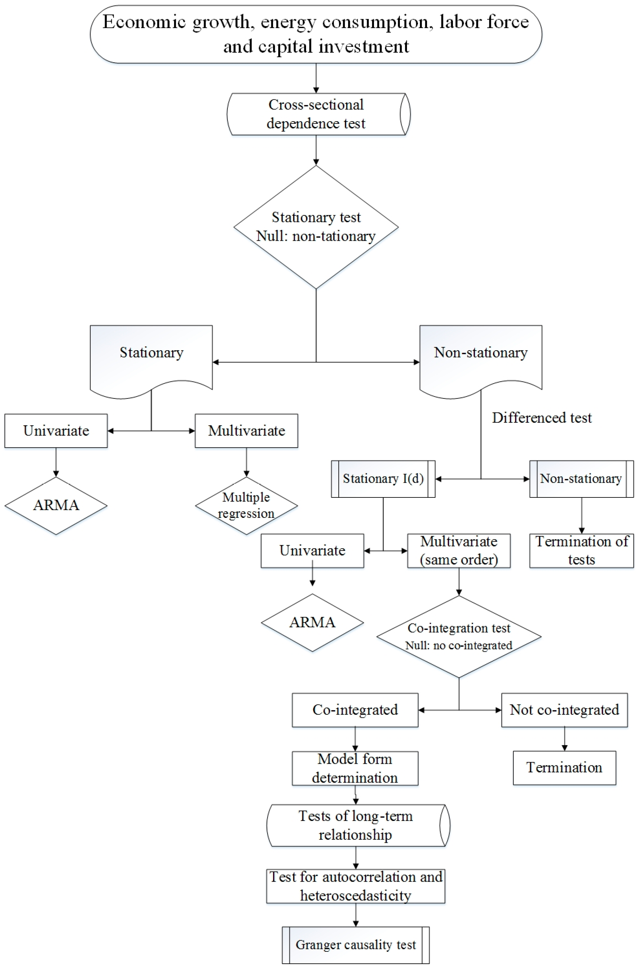
The conceptual framework is illustrated as
Figure 1. The empirical analysis procedure is as follows:
Step 1: Cross-sectional dependence test
Before proceeding with an empirical analysis, a cross-sectional dependence test should be conducted in the panel data model. The existence of cross-sectional dependence determines the method to be used to carry out the unit root test and co-integration test.
Step 2: Unit root test
The second step of this paper is to test the stationarity of these four variables, real GDP, electricity consumption, the input of labor force and capital investment, using the Levin, Lin & Chu (L.L&C) t-test, Im, Pesaran and Shin W-stat (IPS) test, Augmented Dickey Fuller-Fisher (ADF-Fisher) test and Phillips-Perron Fisher (PP-Fisher) test. If the unit root test results show the data sequence is stationary, then regression analysis method will be used to analyze the characteristics of the sequence. If the data series is non-stationary, then differenced test will be employed to determine the order of the series to be stationary. If the series is non-stationary at any order, then the analysis comes to the end. At the stationary order, ARMA is used to analyze univariate, and co-integration test is employed to analyze multivariate which has the same order.
Step 3: Panel co-integration test
If the variables are stationary at the same difference through unit root test, a co-integration test can be carried out. The Pedroni co-integration test is employed here to examine whether there is a long-run equilibrium between these four variables. If the co-integration test results show there is no co-integration relationship, then these series cannot be analyzed. If the co-integration relationship exists, then the analysis will proceed with establishing the panel data model.
Step 4: Model form determination
If the variables are tested to be co-integrated, the likelihood ratio (LR) test, Hausman test and F-test are employed to determine the model form. Then, the panel data model can be estimated.
Step 5: Autocorrelation and heteroscedasticity test
After constructing the panel data model, the Wooldridge test and Breusch and Pagan test method are employed to verify the validity of the established panel data model.
Step 6: Granger causality test
With the aim of further analyzing the relationship between these variables, the Granger causality test can be used to determine the causal relationship and direction between these four variables.
4. Empirical Analysis
4.1. Results of Cross-Sectional Dependence Test
Before proceeding with our empirical analysis, a cross-sectional dependence test should be conducted on the panel data model. The results of Pesaran cross-sectional dependence test are listed in
Table 2. As indicated from the table, the test results accept the null hypothesis for no cross-sectional dependence at 5% level of significance. Therefore, in the procedure of empirical analysis, the cross-sectional dependence across the groups does not need to be taken into consideration. Since we have accepted the null hypothesis, the first-generation unit root tests including Levin, Lin & Chu (L.L&C) t-test, Im, Pesaran and Shin W-stat (IPS) test, Augmented Dickey Fuller-Fisher (ADF-Fisher) test and Phillips-Perron Fisher (PP-Fisher) test can be employed to examine the stationary of different variables.
4.2. Results of Unit Root Test
Before conducting the panel co-integration test to examine the long-term relationship between real GDP, electricity consumption, real total investment in fixed assets and the quantity of employment at the end of the year in the six provinces of North China, it is necessary to examine the stationary of these variables. The unit root test methods commonly used are Levin, Lin & Chu (L.L&C) t-test, Im, Pesaran and Shin W-stat (IPS) test, Augmented Dickey Fuller-Fisher (ADF-Fisher) test and Phillips-Perron Fisher (PP-Fisher) test. The results of the unit root test are listed in
Table 3, which obviously show that these variables are not stationary in their level forms.
Generally, for non-stationary sequences, differenced methods are further employed to identify the stationary of the variables. ΔlnGDP, ΔlnQ, ΔlnK and ΔlnL represent the variables at the first difference. Since the unit root test statistics of all variables are all more than the critical values at the 5% level, all of these variables are stationary at the first difference, which indicate it should reject the null hypothesis of a unit root existing at less than 5% significance level.
4.3. Panel Co-Integration Test Results
Since all of the variables are found to be stationary at the first difference, the analysis will proceed with panel co-integration test by employing Pedroni’s [
7] method which construct seven statistics based on mean values of the individual autoregressive coefficients related to the unit root tests of the residuals of each province in the panel. All these seven tests are distributed asymptotically as standard normal. Monte Carlo simulation results by Pedroni showed that Panel ADF and Group ADF statistics are the most effective. Therefore, according to both Panel ADF-Statistic and Group ADF-Statistic listed in
Table 4, the null hypothesis of no co-integration should be rejected at 5% level of significance.
4.4. Model Form Determination
There are two methods employed for testing the fixed effect and the random effect. One is likelihood ratio (LR) test method used for testing the fixed effect, and the other is Hausman test method used for testing the random effect [
10]. Before estimating the contributions of electricity consumption, real total investment in fixed assets and the quantity of employment at the end of the year to real GDP, these two methods are used to determine whether the model is the fixed effect or the random effect.
The effect test results are shown in
Table 5. As the cross-section
F statistic of LR test is more than the critical value, the null hypothesis that the fixed effect is redundant can be rejected at 5% significance level, that is, the introduction of the fixed effect is appropriate. As the cross-section random statistic of Hausman test is more than the critical value, the null hypothesis that random effect is not related to explanatory variables can be rejected at 5% significance level. Similarly, according to the results of the estimation coefficients of random effect as well as fixed effect and the variance values after difference shown, the model should be the fixed effect model. Then an
F-test will be employed to select the form of the model which includes the variable parameter model, the variable intercept model and the constant parameter model. The software Eviews 6.0 is used to establish models in these three cases and three different sum squared resid values can be obtained, which are set as
S1,
S2 and
S3.
F-test values can be calculated through Equations (28) and (29). If
F1 >
F1,α((
N − 1)
K,(
NT −
N(
K + 1)),
F1,α((
N − 1)
K,(
NT −
N(
K + 1)) is the critical value of the specified significance level), the null hypothesis would be rejected, that means, the panel data model is not the variable intercept model. If
F2 >
F2,α((
N − 1)(
K + 1),(
NT −
N(
K + 1)),
F2,α((
N − 1)(
K + 1),(
NT −
N(
K + 1)) is the critical value of the specified significance level), the null hypothesis should be rejected, that means, the panel data model is not the constant parameter model:
where
N is the number of provinces,
T is the number of periods, and
K is the number of variables. Here,
N = 6.
T = 20,
K = 3.
Table 6 illustrates the F-test results. Since the values of
F1 and
F2 are both greater than the
F values of the specified significance level, the panel data model is a variable parameter model.
4.5. Panel Data Model Estimation
Based on the above test results, we can establish a variable parameter model with fixed effect of real GDP, electricity consumption, real total investment in fixed assets and the quantity of employment at the end of the year in six provinces of North China. The estimated results of the model are listed in
Table 7, which shows that the values of
R2 and adjusted
R2 are 0.9978 and 0.9972, respectively, and the
F statistic is significant. Meanwhile, all the coefficients are positive and significant at the 5% significance level. Therefore, the model is significant, the goodness of fit is high and the model’s effect is perfect.
Given that all the variables are in natural logarithms, the coefficients can be interpreted as elasticities. The estimated results of the model are similar to that of the grey correlation analysis. From the estimated results of the model, we can learn that:
(1) Except for Beijing, the real total investment in fixed assets of other provinces makes the largest contribution to real GDP growth, followed by the electricity consumption. The results imply that a 1% increase in the real total investment in fixed assets increases real GDP by 0.74%, 0.79%, 0.75%, 0.72% and 0.78% in Tianjin, Hebei, Shanxi, Shandong and Inner Mongolia, respectively. Additionally, a 1% increase in electricity consumption increases real GDP by 0.66%, 0.79%, 0.45%, 0.55% and 0.56% in Tianjin, Hebei, Shanxi, Shandong and Inner Mongolia, respectively. As a service industry developed province, the economic growth in Beijing mainly depends on the tertiary industry of which the electricity consumption is larger than other sectors and the input of labor force and capital is smaller than industry. Therefore, a 1% increase in the real total investment in fixed assets has less contribution to real GDP, namely 0.68%, while a 1% increase in electricity consumption has more contribution to real GDP, namely 0.69%.
(2) The contribution of labor force input to real GDP growth is relatively large in the provinces of which the economic growth depends on heavy industry or are less developed. The contribution of the employment level at the end of the year to real GDP growth is larger in Hebei where the industry accounts for a higher proportion and Shanxi, where the economy is relatively backward. A 1% increase of the amount of employment at the end of the year in these two provinces increases real GDP by 0.77% and 0.45%, respectively.
4.6. Results of Autocorrelation and Heteroscedasticity Test
In order to verify the validity of the established panel data model, it is imperative to conduct autocorrelation and heteroscedasticity tests. In this study, Wooldridge test is employed for testing whether there exist autocorrelation between different variables, and Breusch and Pagan test method is applied for examining whether there exist heteroscedasticity between different variables. The results are displayed in
Table 8. As demonstrated in
Table 8, both of autocorrelation and heteroscedasticity tests accept the null hypothesis at 10% level of significance, which mean the established panel data model do not exist autocorrelation and heteroscedasticity. Therefore, the validity of the established panel data model can be verified.
4.7. Granger Causality Test Results
Table 9 introduces the Granger causality test results of which the content with red color means that the null hypothesis should be rejected at the specified level of significance. Taking Beijing as an example, when the null hypothesis is ‘ln
Q does not Granger cause ln
GDP’, the maximum
p value in the brackets of the test is 0.0331 which is smaller than 0.05, thus, the null hypothesis should be rejected. This implies that electricity consumption does Granger cause real GDP. From the results listed in
Table 9, we can obtain that:
(1) There exist bi-directional causal relationships between electricity consumption and real GDP in the six provinces except for Hebei. From the Granger causality test results of the relationship between electricity consumption and real GDP, there is a unidirectional causality running from electricity consumption to economic growth in the six provinces, which means electricity consumption does Granger cause real GDP. Additionally, except for Hebei, there is a unidirectional causality running from economic growth to electricity consumption, which means, real GDP does Granger cause electricity consumption. Except Hebei, other five provinces satisfy the feedback hypothesis that electricity consumption and economic growth are interrelated and mutually complementary. Therefore, the policy of energy conservation and energy structure adjustment will have an influence on economic growth, and the changes in the economic environment will affect electricity demand. The causal relationship between electricity consumption and real GDP of Hebei province satisfy the growth hypothesis that electricity consumption plays a significant role in economic growth, that is, the increase of electricity consumption will promote the growth in real GDP, thus, energy conservation policy will have an adverse effect on economic growth.
(2) Except for Beijing and Hebei, there is a bi-directional relationship between capital input and economic growth as well as labor force input and economic growth. This is because, as a more developed area of service sector, the economic growth of Beijing is highly correlated with electricity demand while the correlation between economic growth and the input of capital and labor force is low. Therefore, there is no causal effect between real GDP and the input of labor force and capital. However, for other industrial area, the economic growth is highly correlated with labor force input and fixed asset input, thus a bi-directional relationship between capital input and economic growth as well as labor force input and economic growth exist in these provinces.
(3) For the whole area of North China, there exists bi-direction causal relationship between real GDP and electricity consumption, real GDP and total investment in fixed assets, and real GDP and the level of employment at the end of the year.
5. Conclusions and Policy Implications
Over the past three decades, China’s economy has witnessed remarkable growth, with an average annual growth rate over 9% [
61]. However, China also faces great challenges to balance its spectacular economic growth and continuously increasing energy use like many other economies in the world [
1]. With the aim of designing effective energy and environmental policies, policymakers are required to master the relationship between energy consumption and economic growth [
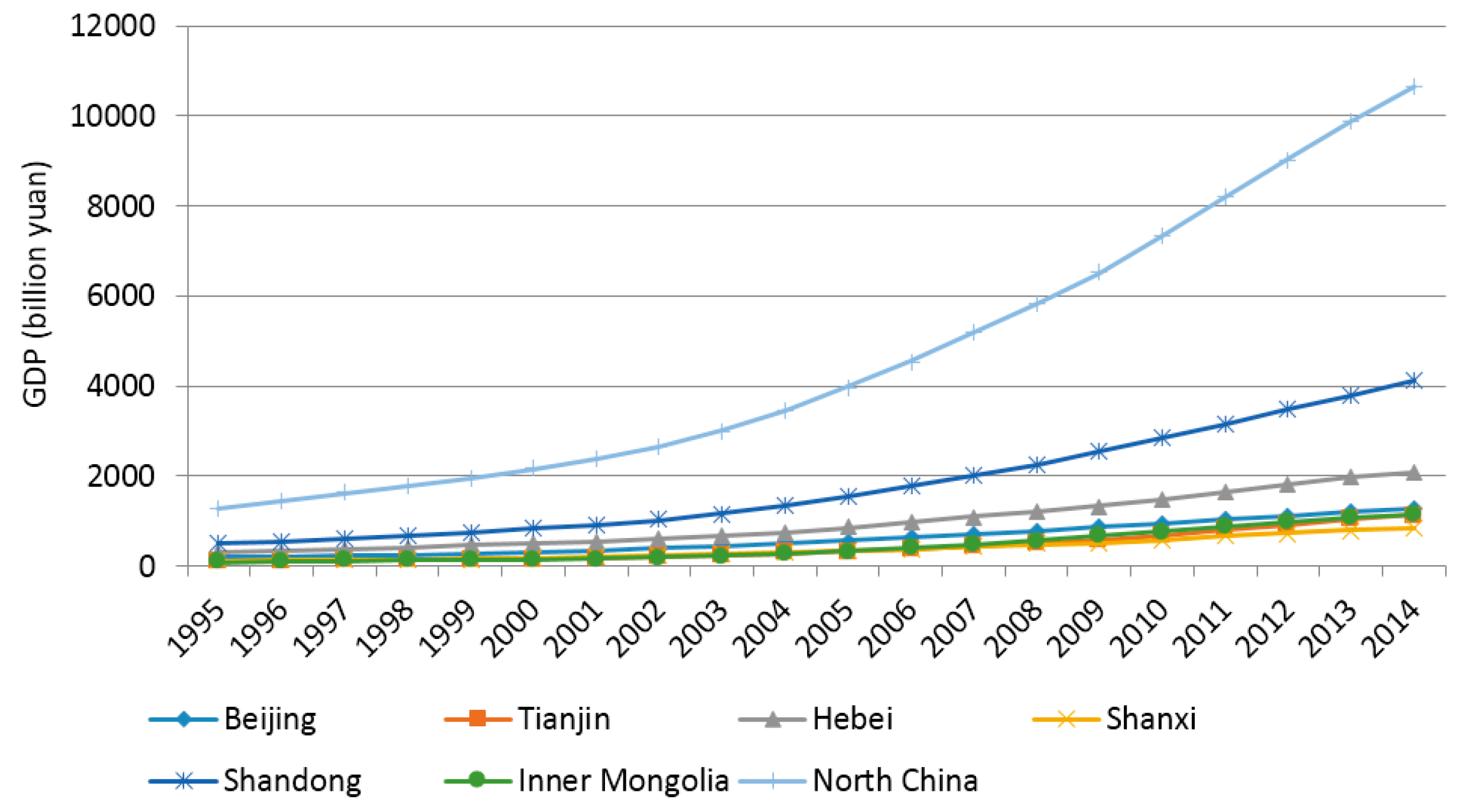
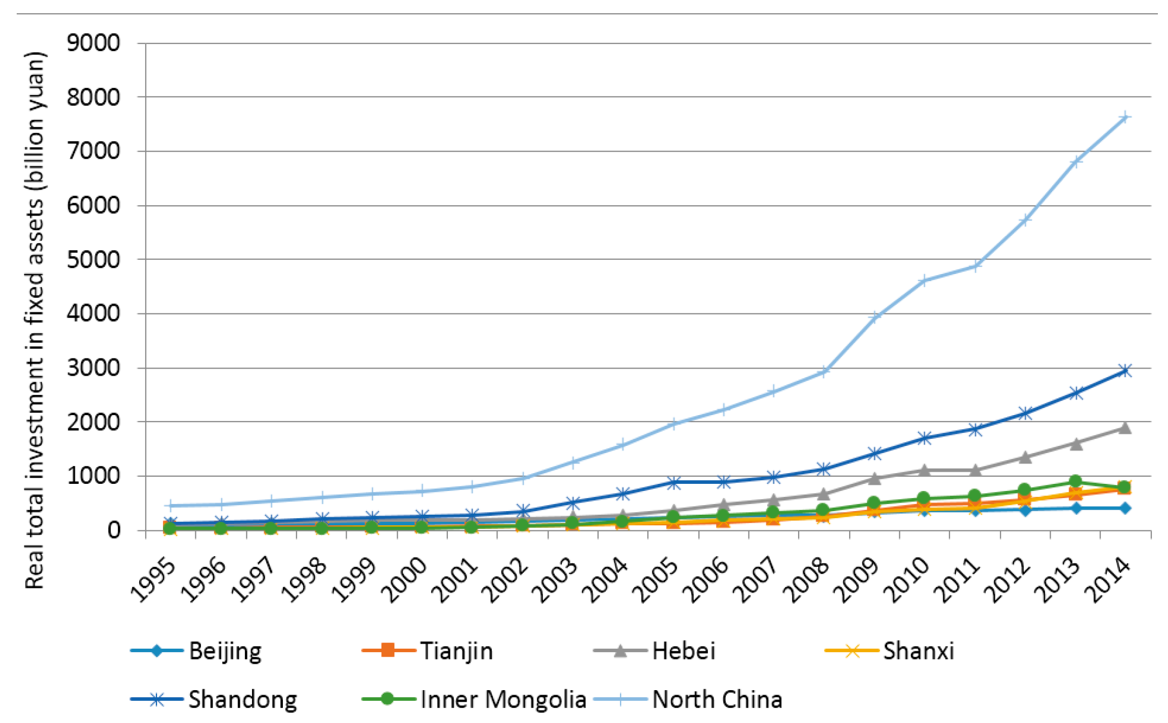
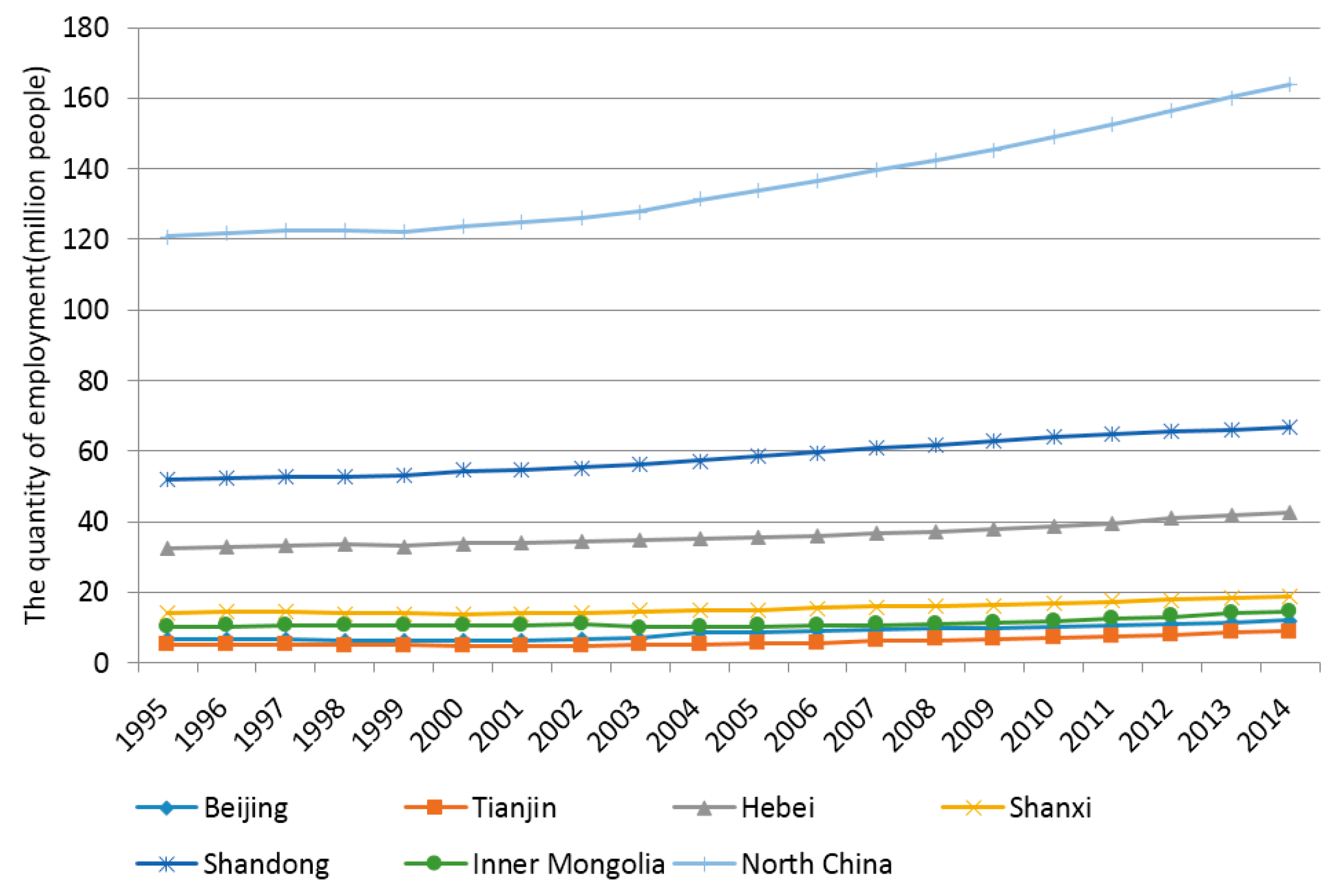
45]. Therefore, in the case of North China, a multivariate model employing panel data analysis method based on the Cobb-Douglas production function introducing electricity consumption as a main factor is established in this paper. The equilibrium relationship and causal relationship between real GDP, electricity consumption, total investment in fixed assets and the quantity of employment at the end of the year are explored using data during the period of 1995–2014 of six provinces in North China, including Beijing, Tianjin, Hebei, Shanxi, Shandong and Inner Mongolia.
The cross-sectional dependence test results illustrated that the cross-sectional dependence across the groups does not need to be taken into consideration. The unit root test results explicitly implied that all variables were non-stationary at level forms but found to be stationary at the first difference, therefore, the null hypothesis ought to be rejected at 5% significance level. Then, the analysis was proceeded with panel co-integration test by employing Pedroni’s panel co-integration test method which stated clearly that all variables were co-integrated in the long term. On the basis of this, the form of the model was determined employing the likelihood ratio (LR) test method and Hausman test method. After establishing the panel data model, the contribution of each factor to the economic growth was analyzed by studying the coefficient of each variable in different provinces. Thus we can obtain that, generally speaking, the real total investment in fixed assets makes the largest contribution to real GDP growth, followed by the electricity consumption. The contribution of labor force input to real GDP growth is relatively large in the provinces of which the economic growth depends on the heavy industry and less developed. Then the Wooldridge test and Breusch and Pagan test method were employed to verify the validity of the established panel data model. In order to further understand the relationship between these variables, Granger causality tests were used to examine the causal relationship between economic growth, electricity consumption and the input of labor force and capital. From the Granger causality tests results, we can learn that there exist bi-directional causal relationships between electricity consumption and real GDP in six provinces except Hebei, and there are bi-directional relationships between capital input and economic growth as well as labor force input and economic growth except Beijing and Hebei.
The empirical results of this study can make policymakers better understand the energy consumption-economic growth nexus to design appropriate energy policies in these provinces. Since electricity consumption Granger causes economic growth, the policy of energy conservation will have an adverse effect on economic growth. However, the stable economic growth should also be guaranteed. Therefore, on the basis of the above econometric analysis, the following suggestions are proposed:
(1) China should reduce energy consumption based on fossil fuels and develop renewable and sustainable energy sources. Proposals for the policy of energy conservation and emission reduction mainly considers the serious pollution originated from the burning of fossil fuel energy. Therefore, it is necessary to reduce the use of energy based on fossil fuels and vigorously develop renewable energy forms, such as wind energy, solar energy and hydro power so that we can not only realize a green GDP growth but also relieve the severe hazy weather in Beijing, Hebei, and other provinces. In the context of the global energy internet, as a region rich of wind energy, Inner Mongolia and Hebei provinces should strive to develop wind power generation systems to make full use of their wind energy resources, and construct transmission networks to deliver the electricity power generated by wind power to Beijing, Tianjin and other provinces.
(2) It is necessary to continually improve energy efficiency and promote the upgrading of economic structure. The provinces of which the development of economy primarily depends on heavy industry should increase the proportion of tertiary industry, especially the modern service industry which has lower energy consumption and higher added value so that the environmental degradation situation can be improved and the hazy weather can gradually be treated. The government should also improve energy saving technology and energy efficiency, and encourage thermal power enterprises to achieve cleaner production.
Therefore, the ways to solve the contradiction of economic growth and energy consumption in North China are reducing energy consumption based on fossil fuel, developing renewable and sustainable energy sources, improving energy efficiency, and increasing the proportion of the tertiary industry, especially the sectors which have low energy consumption and high added value.


