Direct Numerical Simulation of Supersonic Turbulent Boundary Layer with Spanwise Wall Oscillation

Abstract

Direct numerical simulations (DNS) of Mach = 2.9 supersonic turbulent boundary layers with spanwise wall oscillation (SWO) are conducted to investigate the turbulent heat transport mechanism and its relation with the turbulent momentum transport. The turbulent coherent structures are suppressed by SWO and the drag is reduced. Although the velocity and temperature statistics are disturbed by SWO differently, the turbulence transports of momentum and heat are simultaneously suppressed. The Reynolds analogy and the strong Reynolds analogy are also preserved in all the controlled flows, proving the consistent mechanisms of momentum transport and heat transport in the turbulent boundary layer with SWO. Despite the extra dissipation and heat induced by SWO, a net wall heat flux reduction can be achieved with the proper selected SWO parameters. The consistent mechanism of momentum and heat transports supports the application of turbulent drag reduction technologies to wall heat flux controls in high-speed vehicles.

1. Introduction

Aerodynamic heating is an inherent feature of supersonic and hypersonic flights, bringing out lots of problems, such as the increase of infrared radiation, the decrease of rigidity and intensity of aircraft structures, and even material ablation. Therefore, it is one of the most important problems in designing high-speed vehicles, such as hypersonic aircraft and reentry spacecraft [1]. What is more, aerodynamic heating is remarkably increased when the boundary layer transits from laminar status to turbulent status [2]. To protect the high-speed vehicle from burning down, a thermal protection system, although regarded as a dead weight in terms of aerodynamic performance, is required. Therefore, the reduction of wall heat flux (WHF) as a way of lessening the aerodynamic heating becomes critical in the development of high-speed vehicles.

Compared with WHF control, the research in an effort to realize drag reduction has been conducted with abundant satisfactory achievements, due to its significance in energy saving. Research on wall heat flux properties in incompressible flows with drag reducing devices has also been performed [3,4,5]. Although the major target of these studies was to find a way of enhancing surface heat flux to improve heat exchangers’ performance, they always obtained the consistent changes of WHF and drag. However, these studies shed light on the idea of reducing WHF by applying drag reduction control methods in the present paper.

Spanwise wall oscillation (SWO), as one of the active boundary layer control methods, has been extensively studied due to its effectiveness in suppressing turbulence and drag reduction as well as its close relation with wall turbulence regeneration mechanism. The first SWO research was done numerically in the channel flow by Jung et al. [6] with a maximum drag reduction of 40% attained. This was then proved in the water channel experiment conducted by Laadhari et al. [7], who reported that the mean velocity gradient of the turbulent boundary layer was decreased for $y^{+}<8$. Laadhari et al. [7] demonstrated that the conclusions obtained by Jung et al. [6] are corresponding with those in the boundary layer flow for the first time. It has been confirmed that, no matter in channelflow [6,7,8] or boundary layer flow [9,10], the linear sub-layer of the velocity profile is thickened and the log-law layer is shifted upward when the drag is reduced by SWO. The characteristic of the spatial transient in the boundary layer flow has to be taken into account, i.e., the local skin friction drag decreases to the maximum value even beyond a few thousands of wall units downstream from the leading edge of the oscillation, as reviewed by Quadrio [11]. The drag reduction of as much as 45%, the same order as Jung et al. [6] obtained, was observed within five boundary-layer thicknesses downstream of the start of wall oscillation, as reported by Choi et al. [9]. The Reynolds stresses in boundary layer flows are also found to be suppressed by SWO [7,10,12,13] and the magnitude of the reduction was qualified by Skote [14]. Many studies have focused on the optimization of the oscillating parameters. Given the implicit oscillating parameter, namely the maximum displacement of the wall, two optimal periods, i.e., one at fixed displacement and the other one at fixed amplitude were suggested by Quadrio and Ricco [15], and the latter one was subsequently confirmed by Ricco and Quadrio [16]. Although external energy is required to drive the wall motion, overall energy saving can be achieved by optimizing the oscillation parameters. Baron and Quadrio [8] and Quadrio and Ricco [15] have demonstrated that a net energy saving of 7% or more could be reached with proper oscillation parameters. Hasegawa et al. [17] proposed a constant power input (CPI) concept for turbulent duct flows and applied this in DNS of low-Reynolds-number channel flow with SWO. They obtained 90% of the available power for the pumping system and the remaining 10% for the control system to yield the largest increase of the flow rate.

The heat transport property in the weakly compressible channel flow with SWO was studied by Fang et al. [18,19]. They concluded that the consistency of the mechanisms between heat and momentum transports is preserved and a 5% mean WHF reduction was obtained via setting appropriate oscillating SWO parameters. Due to the essentially incompressible characteristic of the cases studied by Fang et al. [18,19], it is still not very clear whether their conclusion still holds in high-speed flows. Therefore, it is necessary to investigate the SWO in the supersonic turbulent boundary layer to explore the turbulent heat transport mechanism, especially its relation with momentum transport. The results reached would be more significant for the development of wall heat flux control technologies in high-speed vehicles.

In the present paper, the supersonic spatial developing boundary layer disturbed by SWO with different amplitudes and frequencies is studied using direct numerical simulation (DNS) and a special focus has been put on the turbulent heat transport mechanism. The relation between momentum transport and heat transport is particularly analyzed to bring insight into their consistency not being disturbed by control devices. In Section 2, we describe the governing equations, the numerical method and the setup of cases. The results are validated and the flow fields are analyzed in Section 3. Finally, in Section 4 we draw some conclusions.

2. Methodologies

2.1. Governing Equations

The three-dimensional unsteady compressible Navier-Stokes (N-S) equations in a general, time-invariant system are solved numerically. The N-S equations are non-dimensionalized with the reference velocity $u_{ref}$, temperature $T_{ref}$, density ${\rho }_{ref}$ and dynamic viscosity ${\mu }_{ref}$ of the incoming free stream flow and the reference length scale ${\delta }_{ref}$, which is the nominal thickness of the turbulent boundary layer at the leading edge of the flat plate. The resulting dimensionless parameters are the Reynolds number $Re={\rho }_{ref}{u}_{ref}{\delta }_{ref}/{\mu }_{ref}$ and the Mach number $M=u_{ref}/\sqrt{\gamma R{T}_{ref}}$. A constant Prandtl number $Pr=\mu C_p/k=0.72$ is used, where $C_p=\gamma R/\left(\gamma -1\right)$ is the specific heat capacity of gas at constant pressure and $k$ is the thermal conductivity. The parameters R and $\gamma$ are the gas constant and the specific heat capacity ratio, which are set to be R = 287.1J/(kg·K) and $\gamma =1.4$, respectively. This set of N-S equations can be written in a strong conservation form as:

$$\frac{\partial \mathit{Q}}{\partial t}+\frac{\partial {\mathit{E}}_i}{\partial x_i}=\frac{\partial {\mathit{F}}_i}{\partial x_i}$$

(1)

In Equation (1), $\mathit{Q}={\left[\rho ,\rho u,\rho v,\rho w,E\right]}^{\mathrm{T}}$ is the solution vector. The primary variables are the density $\rho$, the velocity components u, v and w and the total energy E. The static temperature T and the pressure P are related to the density $\rho$ via the equation of state of the ideal gas $P=\rho T/\left(\gamma M^2\right)$.

The convection terms ${\mathit{E}}_i$ and the diffusion terms ${\mathit{F}}_i$ in Equation (1) are, respectively, expressed as:

$${\mathit{E}}_i=\left[\begin{array}{c}\rho u_i\\ \rho u{u}_i+{\delta }_{1i}P\\ \rho v{u}_i+{\delta }_{2i}P\\ \rho w{u}_i+{\delta }_{3i}P\\ \left(E+P\right)u_i\end{array}\right],{\mathit{F}}_i=\left[\begin{array}{c}0\\ {\tau }_{1i}\\ {\tau }_{2i}\\ {\tau }_{3i}\\ b_i\end{array}\right]$$

(2)

with the standard Einstein summation notation. The notations $x_i$ and $u_i$ (i = 1, 2, 3) are adopted to represent (x, y, z) and (u, v, w) respectively. ${\delta }_{ij}$ is the standard Kronecker delta.

The total energy E is expressed as:

$$E=\frac{1}{2}\left(\rho u_i{u}_i\right)+\frac{\rho T}{\gamma \left(\gamma -1\right)M^2}$$

(3)

The stress tensor and the heat flux vector are expressed as:

$${\tau }_{ij}=\frac{\mu }{Re}\left(\frac{\partial u_i}{\partial x_j}+\frac{\partial u_j}{\partial x_i}-\frac{2}{3}{\delta }_{ij}\frac{\partial u_k}{\partial x_k}\right)$$

(4)

and

$$b_i=u_j{\tau }_{ij}+\frac{\mu }{PrRe\left(\gamma -1\right)M^2}\frac{\partial T}{\partial x_i}$$

(5)

The dynamic viscosity coefficient $\mu$ is calculated via the Sutherland law:

$$\mu =T^{1.5}\frac{T_S/T_{ref}+1}{T+T_S/T_{ref}}$$

(6)

where $T_{ref}=104.4\text{K}$ and $T_S=110.4\text{K}$.

2.2. Numerical Method

Equation (1) is projected to the coordinate system of the computational domain and solved with the high-order finite difference method. All the spatial derivatives are approximated with the classic sixth-order compact central scheme proposed by Lele [20].

The derivatives of the diffusion terms are solved with double applications of the first-order difference. The primitive velocity components $u_i$ and temperature variable T are firstly differentiated to formulate the stress tensor and the heat flux vector at each node point. The diffusion terms are then computed with another application of the sixth-order compact scheme. This method is more efficient than the direct calculation of the second-order derivatives [21], although the latter method could be numerically more stable. To remove the small-scale wiggles due to aliasing errors resulting from discrete evaluation of the nonlinear convection terms, the tenth-order compact filter is incorporated, which limits the filtering only at high wave numbers [22]. After all the spatial terms are solved, the third-order total variation diminishing (TVD) Runge-Kutta method [23] is used for the time integration.

2.3. Computational Setup

The sketch of the case studied is demonstrated in Figure 1. The wall is divided into a non-moving wall and an oscillating wall as well as a transitional zone between them. The isothermal non-slip boundary condition is applied at the wall with the spanwise wall velocity given as:

$$W_w=W_{m}f\left(x\right)\sin \left[2\mathsf{\pi }\frac{t}{t_{osc}}\right]$$

(7)

where $W_m$ is the amplitude of the wall velocity and $t_{osc}$ is the period of wall oscillation. $f\left(x\right)$ is a function describing the transitional zone as:

$$f\left(x\right)=S\left(\frac{ x -x_{start}}{\Delta x_{rise}}\right)$$

(8)

$x_{start}$ and $\Delta x_{rise}$ are the start position and the length of the transitional zone, respectively, which are set as $x_{start}=27.975$ and $\Delta x_{rise}=2.0$. $S\left(x\right)$ is a continuous step function that rises from zero for $x\le 0$ to unity for $x\ge 1$ with the advantage of owning continuous derivatives of all orders,

$$S\left(x\right)=\{\begin{array}{c}0\\ 1/\left(1+{\mathrm{e}}^{\left(1/\left(x-1\right)+1/x\right)}\right)\\ 1\end{array}\begin{array}{c}x\le 0 \\ 0<x<1\\ x\ge 1 \end{array}$$

(9)

Similar transitional function was also adopted by Yudhistira and Skote [24] as well as Skote [14].

The Mach number of the incoming free stream flow is M = 2.9 and the Reynolds number is set as Re = 16,265.8.

The size of the computational domain is $49{\delta }_0\times 4{\delta }_0\times 5{\delta }_0$ and it is discretized via a mesh with $1980\times 120\times 400$ points in x, y and z directions. The mesh is uniformly distributed in x and z directions and stretched towards wall in the y direction. The mesh’s resolution in the fully developed region without SWO is $\Delta x^{+}=12.5$, $\Delta y_1^{+}=0.9$ and $\Delta z^{+}=6.2$, which matches the requirement for DNS of wall turbulence proposed by Sagaut [25]. The time step of the computation in the present study is 0.004.

The digital filter method proposed by Touber and Sandham [26] is used to generate synthetic inflow turbulence and a transitional region of $12{\delta }_0$ is incorporated to make synthetic fluctuations evolve into fully developed turbulence. The generated artificial turbulent fluctuations are super-imposed onto the mean velocity and temperature profiles. The supersonic inflow condition is then adopted to prescribe the flow variables at the inlet plane, except in the subsonic portion of the boundary layer, where the pressure is extrapolated from the inner grid points. At the upper and the outlet planes, the generalized non-reflecting boundary conditions [27,28] are used.

The wall temperature is set as $T_w=1.5T_0$, which is a cold wall comparing with the adiabatic wall temperature $T_r=2.43T_0$ calculated via:

$$T_r=T_0\left(1+r\frac{\gamma -1}{2}{M}^2\right)$$

(10)

with the recovery coefficient being $r=\sqrt{Pr}$.

Fourteen cases are studied including the baseline Case 0 with a non-moving wall. The wall oscillation parameters are listed in

Table 1. Parameters of the wall oscillation.

Group	Case	${\mathit{t}}_{\mathit{o}\mathit{s}\mathit{c}}^{\mathbf{+}}$	${\mathit{W}}_{\mathit{m}}^{\mathbf{+}}$	No. of Samples
0	0	∞	0	2000
1	P50A3	50	3	1640
	P100A3	100	3	1680
	P150A3	150	3	2120
	P200A3	200	3	1800
	P250A3	250	3	1760
	P300A3	300	3	1720
	P400A3	400	3	1720
2	P150A1	150	1	2120
	P150A1.5	150	1.5	2120
	P150A3	150	3	2120
	P150A5	150	5	2120
	P150A7	150	7	2120
	P150A10	150	10	2120
	P150A20	150	20	2120

, in which $t_{osc}^{+}$ and $W_m^{+}$ are the period and amplitude of SWO in the inner scale, calculated via

$$t_{osc}^{+}=\frac{t_{osc}{\rho }_w{u}_{\tau }^2}{{\mu }_w}Re$$

(11)

and

$$W_m^{+}=W_m/u_{\tau }$$

(12)

in which $u_{\tau }$ is taken from the baseline case at $x=x_{start}$.

The cases with SWO are categorized into two groups. The cases in Group 1 have the same wall oscillation amplitude of $W_m^{+}=3$ and the cases in Group 2 have the same oscillation period of $t_{osc}^{+}=150$. Therefore, the effects of period and amplitude are respectively studied in the two groups. After the early transition period, the simulation reached the statistically stationary status. Then the data were collected every 50 time steps for the calculations of flow statistics. The numbers of samples are slightly different for cases, as presented in Table 1. The uncertainty related to the averaging time is estimated using the method proposed by Gatti and Quadrio [29], and a 1.5% uncertainty could be generally achieved for the studied cases.

3. Results and Discussion

3.1. Validation

The DNS results are validated by comparing Case 0 with available boundary layer data from both measurements and other DNS. The mean flow variables are calculated via the Favré average, defined as $\langle f\rangle =\overline{\rho f}/\overline{\rho }$, in which $f$ is a general variable and “$\stackrel{-}{ }$” stands for the mean value. The fluctuations are then defined as $f″=f-\langle f\rangle$ and $f\prime =f-\overline{f}$. The mean velocity profile handled by the Van Driest transformation at $x=x_{start}$ in the inner scale is compared with the classic incompressible law of wall and experimental data [30,31], as well as some results from DNS of supersonic boundary layers [32,33,34] in Figure 2. A good agreement between the present DNS and other data in the linear sub-layer and log-law layer is obtained. The difference in the wake layer is attributed to the Reynolds number effects [35].

According to the Morkovin’s hypothesis, the density-scaled root mean square (RMS) velocity fluctuations $u_{i,DRMS}^{″}=\sqrt{\frac{\overline{\rho }}{{\overline{\rho }}_W}\langle u_i^{″}{u}_i^{″}\rangle }$ of Case 0 at $x=x_{start}$ are compared with the low Reynolds number boundary layer experimental data [31,36], incompressible DNS [37,38], compressible DNS at transonic speed [39], and DNS of supersonic boundary layer at Mach number of 2.5 [33,34] as indicated in Figure 3. $u_{i,DRMS}^{″}$ are normalized with the friction velocity $u_{\tau }$. A general good agreement for RMS velocity fluctuations can be seen in the near-wall region. However, high values of velocity fluctuations can be seen beyond the peak for the present case. According to the study of Duan et al. [40], with a higher Mach number and lower wall temperature, the velocity fluctuations get larger values after the peak. Therefore, the higher values of RMS velocity fluctuations are attributed to the cold wall condition adopted in the present research.

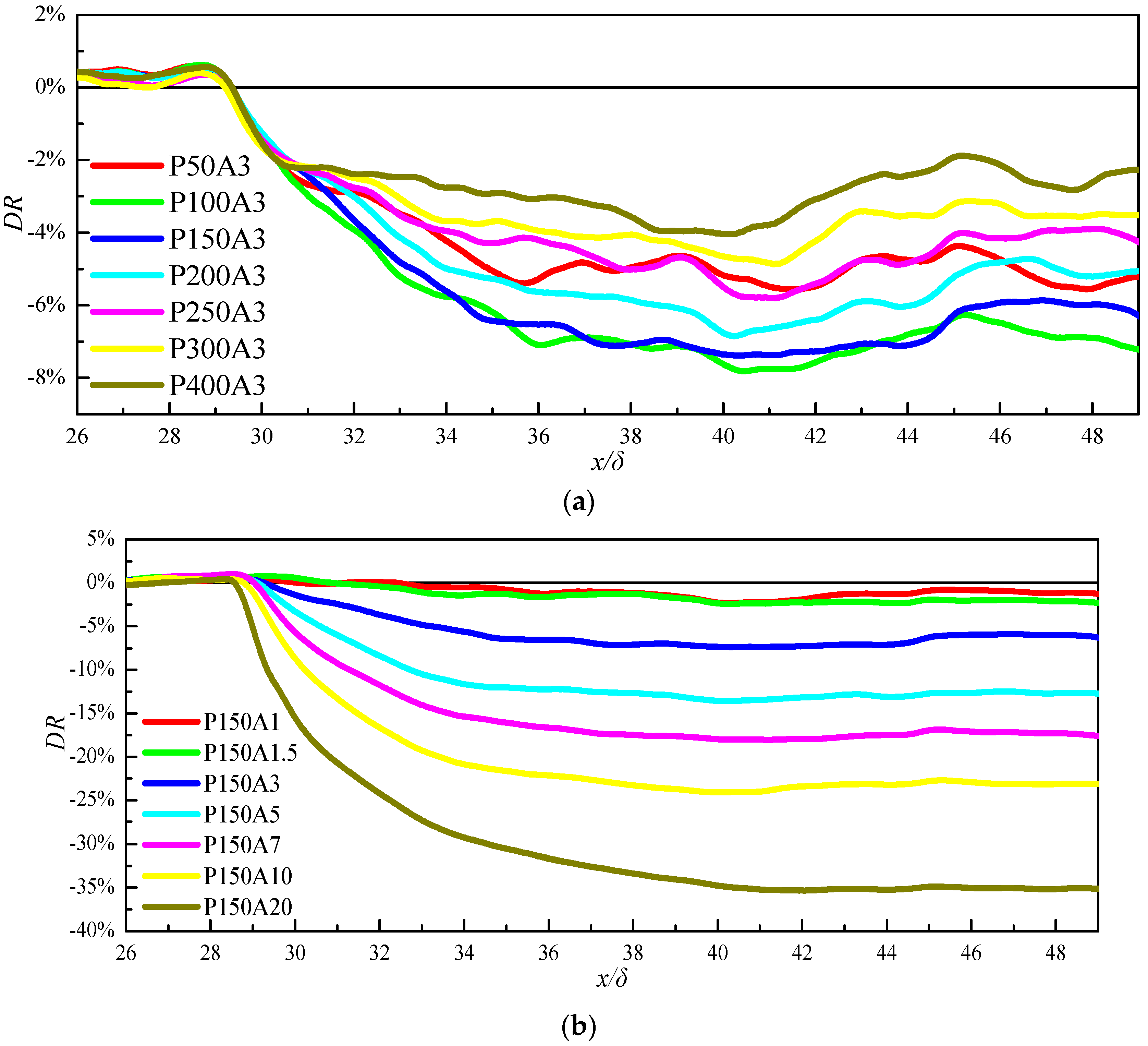
3.2. Drag and Wall Heat Flux

The results obtained with SWO are presented below. The next figures present general effects of SWO on the turbulent structures. The turbulent coherent structures visualized with the iso-surface of the swirling strength ${\mathsf{\lambda }}_{ci}$ [41] and the near-wall velocity fluctuations at the x-z plane of $y^{+}=10$ of Case P150A20 are shown in Figure 4, from which we can see the effective disturbance of near-wall coherent structures by SWO. According to Figure 4a, beyond $x_{start}$, the density of the horseshoe vortex in the boundary layer is weakened, indicating the turbulent coherent structures are suppressed. In the upstream undisturbed boundary layer, the near-wall velocity fluctuations present classic streamwise elongated streaky structures. The streaks are dramatically disturbed by SWO downstream. The direction of streaks changes with the wall movement and their configuration gets distortion. Their strength is weakened, and the distance between neighboring streaks is also increased. Therefore, the mode of the modification of wall turbulence by SWO in the present supersonic boundary layer flow is similar with that of the incompressible flows [42].

The rates of the change of drag (DR) and wall heat flux (HR) are defined as:

$$DR\left(x\right)=\frac{{\tau }_w\left(x\right)-{\tau }_{w0}\left(x\right)}{{\tau }_{w0}\left(x\right)}\times 100\%$$

(13)

and

$$HR\left(x\right)=\frac{q_w\left(x\right)-q_{w0}\left(x\right)}{q_{w0}\left(x\right)}\times 100\%$$

(14)

where ${\tau }_w={\mu }_w{\frac{\partial <u>}{\partial y}|}_w$ and $q_w=k_w{\frac{\partial <T>}{\partial y}|}_w$ are the wall shear stress and wall heat flux. Therefore, positive DR and HR mean the increase of drag and wall heat flux and vice versa. DR and HR of all the controlled cases are plotted in Figure 5 and Figure 6. The peak values of DR and HR for each case are listed in

Table 2. Peak values of DR and HR.

Group	Case	Min DR	Max HR	Min HR	Corrected Min HR
1	P50A3	−6%	10%	6%	−7%
	P100A3	−8%	5%	0%	−9%
	P150A3	−7%	4%	−2%	−9%
	P200A3	−7%	3%	−2%	−8%
	P250A3	−6%	2%	−2%	−7%
	P300A3	−5%	2%	−2%	−6%
	P400A3	−4%	2%	−1%	−5%
2	P150A1	−2%	1%	−2%	−3%
	P150A1.5	−2%	2%	−1%	−3%
	P150A3	−7%	4%	−2%	−9%
	P150A5	−14%	10%	3%	−17%
	P150A7	−18%	22%	15%	−24%
	P150A10	−24%	52%	44%	−34%
	P150A20	−35%	248%	242%	−53%

.

It can be seen in Figure 5 that the drag is effectively reduced for all the cases. Comparing the two groups, we can observe that DR changes monotonically with the SWO amplitude and non-monotonically with the SWO period. Therefore, for Group 1, the optimized period for the maximum drag reduction is in the range of $t_{osc}^{+}=100~150$, close to the optimized period of $t_{osc}^{+}=100~125$ in the incompressible channel flow [15]. About 8% drag reduction is achieved for Case P100A3 at $x=40$, also agreeing well with the 11% drag reduction gained in the incompressible channel with $t_{osc}^{+}=125$ and $W_m^{+}=3$ [18]. For Group 2 with the nearly optimized period of $t_{osc}^{+}=150$, a maximum drag reduction of 35% is obtained for the case with the largest amplitude, corresponding to the maximum drag reduction of 40% obtained by Jung et al. [6] in the incompressible channel. It can be concluded that the drag reduction property of SWO in the supersonic boundary layer flow is consistent with that in the incompressible channel flow, indicating the compressibility effect might not have a major influence on SWO in terms of the drag reduction.

Based on the HR shown in Figure 6, WHF is increased in most cases, because of the shear of the spanwise Stokes layer acting as a heat source on the temperature field. Therefore, generally, with a higher frequency and larger amplitude of SWO, a higher WHF can be obtained. Consequently, Case P150A20, although the maximum DR is realized, has the WHF increased by nearly 250% due to the massive dissipation induced by the spanwise Stokes shear layer. However, for the cases with lower frequency and smaller amplitude ($T^{+}\ge 100$ and $W_m^{+}\le 3$), a reduction of WHF can still be acquired, mainly because of the combined effects of the suppression of turbulence transport and the reduction of the shear of streamwise velocity [18,19]. About 2% maximum WHF reduction can be attained for $t_{osc}^{+}=150$ and $W_m^{+}=3$ comparing with 5% WHF reduction obtained in the Mach = 0.5 channel flow [18]. The maximum WHF reduction takes place at about $x=40$, which is the same location where the maximum drag reduction is attained, implying the consistent effects of SWO on drag and WHF.

To investigate the influence of the Stokes layer on the WHF, the solution of one dimensional (1D) laminar Stokes layer is used to estimate the temperature field and WHF. According to previous research in SWO [43,44,45], the near-wall spanwise velocity profile agrees well with the laminar Stokes solution, even though the main flow is fully turbulent. We are considering a static fluid in a space with a half-infinite spanwise oscillating wall. The spanwise speed of the wall is given as $W_w=W_m\sin \omega t$. Then the N-S equations can be simplified as,

$$\frac{\partial }{\partial t}w\left(y,t\right)=\frac{\mu }{\rho Re}\frac{{\partial }^2}{\partial y^2}w\left(y,t\right)$$

(15)

$$\frac{\partial }{\partial t}T\left(y,t\right)=\frac{\gamma \left(\gamma -1\right)M^2}{\rho Re}{\left[\frac{\partial }{\partial y}w\left(y,t\right)\right]}^2+\frac{\mu \gamma }{\rho RePr}\frac{{\partial }^2}{\partial y^2}T\left(y,t\right)$$

(16)

It can be seen that Equation (16) is a simple 1D thermal diffusion equation and the spanwise Stokes velocity layer acts only as a source term. According to Equation (16), the heat source of the Stokes layer will be larger with the increase of the Mach number. Therefore, WHF should be further increased with a higher Mach number. Regarding the effect of Prandtl number $Pr$, it has an inverse relation to the thermal diffusivity. Considering the source term being always positive in the present case, larger $Pr$ will cause smaller WHF and vice versa.

Equations (15) and (16) can be easily numerically solved with the same method of solving N-S equations in Section 2.2. Isothermal non-slip boundary condition and extrapolation method are adopted at the wall and upper boundary respectively. The temporal evolution of the WHF $q_w\left(x\right)$ solved from the Stokes equations is presented in Figure 7, along with spanwise averaged WHF results from Case P150A20 and Case 0 at x = 40.775. The strong temporal fluctuation of WHF of Case P150A20 is in a good phase consistency with the result of the laminar Stokes solution, although the WHF of Case P150A20 has larger peak values due to the contribution of the streamwise flow motion. The corrected WHF is then calculated by subtracting the Stokes solution from the overall WHF and the turbulence-like fluctuation of WHF can be recovered. The corrected WHF can be assumed to be the part contributed from the streamwise flow motion and we can get that it gets reduced relative to that of the undisturbed Case 0.

Despite this linear correction being debatable, it is worth seeing the wall heat flux ratio by removing the part of the laminar Stokes solution, denoted as corrected HR plotted in Figure 8. The corrected HR is defined as:

$$HR\left(x\right)=\frac{q_w\left(x\right)-q_{ws}\left(x\right)-q_{w0}\left(x\right)}{q_{w0}\left(x\right)}\times 100\%$$

(17)

in which $q_{ws}\left(x\right)$ is the wall heat flux calculated from the Stokes solution.

As illustrated in Figure 8, we can find a consistent trend between corrected HR and DR in Figure 5, especially for the cases with small SWO amplitudes. This further confirms that the increase of WHF is mainly due to the Stokes layer, as mentioned above. For cases with large amplitudes, negative peaks downstream of the location where SWO started can be identified. These peaks should be attributed to the Stokes layer being still in development. Consequently, the increase of the WHF of DNS is lower than that of the Stokes solution, as presented in Figure 9. Therefore, the subtraction of the Stokes solution from the DNS result would cause the over-correction of WHF.

The values of corrected HR at the locations of minimal HR of each case are also presented in Table 2. Similar levels of the reduction of corrected HR and DR can be seen, although the correction is not very accurate for cases with large amplitudes.

In the following part of the paper, Cases 0, P150A20 and P150A3 as representatives of undisturbed case, the maximum disturbed case, and the WHF reduction case respectively will be analyzed in details.

3.3. Mean Profiles

The mean streamwise velocity profiles at x = 40.775 for the three cases are presented in Figure 10. The x = 40.775 is the location where the SWO gets its maximum effects according to the analysis above.

According to Figure 10a, it is clear that the SWO causes a decrease of the mean velocity within $y<0.1\delta$. Therefore a thinner velocity profile is formed corresponding to a lower skin friction. The velocity profile in the local inner scale as manifested in Figure 10b presents an extended linear sub-layer and a higher log-law layer, which is a general characteristic of drag reducing flows [6,7,8,9].

Mean temperature profiles at x = 40.775 for the three cases are presented in Figure 11. A temperature peak around $y=0.02\delta$ can be observed for all the cases due to the cold wall condition adopted in the present research, which have a critical influence on temperature statistics. As the result of the dissipation of the Stokes layer, a great increase of the peak value of the mean temperature appears in Case P150A20 and we can see that the effect of the Stokes layer on the mean temperature profile is mainly limited in the region of $y<0.3\delta$. In the zoomed figure of the near-wall region inside Figure 11, a slight reduction of the mean temperature for Case P150A3 can be observed, which causes the reduction of mean WHF.

The velocity and temperature fluctuation intensities are plotted in Figure 12 and Figure 13. The wall friction velocity $u_{\tau }$ and friction temperature $T_{\tau }$ at $x_{start}$ of Case 0 is used to normalize velocity and temperature variables. The reason of using the same friction velocity and temperature as references for all cases is to highlight the absolute changes of turbulence fluctuations under the influence of SWO. According to the research of Baron and Quadrio [8] and Hasegawa et al. [17], the suppression of turbulence intensity may be not so obvious when the actual local friction velocity is adopted.

The velocity fluctuation intensities for both the controlled cases are weakened and it is clear that the case with larger oscillation amplitude gets a greater suppression of velocity fluctuations. The steep rise of spanwise velocity intensity in the near-wall region seen in Figure 12c is due to the simple ensemble averaging procedure (rather than phase averaging) being adopted to process the periodicity of the spanwise Stokes layer.

It can be seen in Figure 13 that the temperature fluctuation intensities are also altered by SWO. Contrary to the consistent decrease of velocity fluctuation intensities of both the cases, the turbulent temperature fluctuation intensity of Case P150A3 is slightly reduced except in the region marked by the two red lines, while the temperature fluctuation of Case P150A20 is seriously amplified and a strong peak is created at about $y^{+}\approx 35.6$. It is also attributed to the unsteady Stokes layer, which causes the periodic change of the temperature field regarded as temperature fluctuations. In Figure 13b, we can find near-wall peaks for all the cases at about $y^{+}\approx 4.1$. Those peaks are related to the strong temperature gradient in the near-wall region between the mean temperature peak and wall, as presented in Figure 11.

According to the analysis above, it looks that the velocity statistics and the temperature statistics get completely different influences from SWO. However, the following analysis will demonstrate that the underline transport mechanisms are consistent.

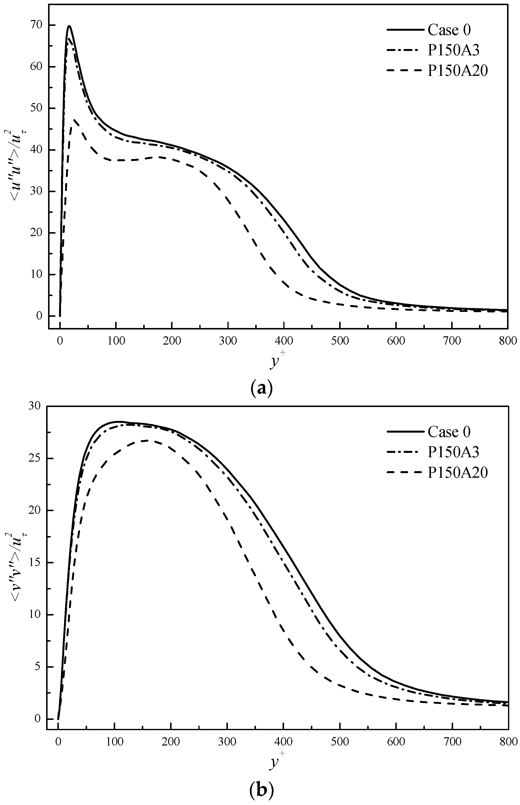
3.4. Transport Properties

The Reynolds shear stress $\langle u^{″}{v}^{″}\rangle$ and normal turbulent heat flux $\langle T^{″}{v}^{″}\rangle$, standing for the turbulent momentum and heat transport capacities respectively are plotted in Figure 14. In addition, the same reference friction velocity and friction temperature of Case 0 are used for the normalization. Figure 14a shows that $\langle u^{″}{v}^{″}\rangle$ of both the two controlled cases are reduced and a greater suppression is acquired with a larger SWO amplitude. As a result, the drag is reduced at the level of 7% and 35% for Case P150A3 and P150A20, respectively, indicating a close correlation between the suppression of momentum transport and drag reduction.

It can be seen in Figure 14b that $\langle T^{″}{v}^{″}\rangle$ of Case P150A3 is suppressed in almost the entire boundary layer and $\langle T^{″}{v}^{″}\rangle$ of Case P150A20 is slightly suppressed in most places except a limited region between the two red lines. With the zoomed figure of Figure 14c, we can see $\langle T^{″}{v}^{″}\rangle$ alters from positive to negative values when approaching the wall at the peak location of the mean temperature profile as shown in Figure 11. This can be explained by the change of the mean temperature gradient. Still, the near-wall turbulent heat transports are suppressed by SWO for the two cases. Comparing the two controlled cases, the one with larger amplitude gets a greater reduction of $\langle T^{″}{v}^{″}\rangle$, which is consistent with its effects on $\langle u^{″}{v}^{″}\rangle$.

The cross correlations of $\langle u^{″}{v}^{″}\rangle$ and $\langle T^{″}{v}^{″}\rangle$ are analyzed to study the influence of the turbulent structures on turbulent transports. The cross correlations $R\left(u″,v″\right)$ and $R\left(T″,v″\right)$ are, respectively, defined as:

$$R\left(u″,v″\right)=\frac{\langle u^{″}{v}^{″}\rangle }{\sqrt{\langle u^{″}{u}^{″}\rangle \langle v^{″}{v}^{″}\rangle }},$$

(18)

and

$$R\left(T″,v″\right)=\frac{\langle T^{″}{v}^{″}\rangle }{\sqrt{\langle T^{″}{T}^{″}\rangle \langle v^{″}{v}^{″}\rangle }}.$$

(19)

Their profiles at x = 40.775 are plotted in Figure 15. For both $R\left(u″,v″\right)$ and $R\left(T″,v″\right)$, we can identify a near-wall peak for Case 0, which stands for the contribution of certain organized turbulence motions in the near-wall region, as proposed by Kim et al. [46] for the incompressible channel flow. The strength of the near-wall peaks of $R\left(u″,v″\right)$ is effectively suppressed due to the restrain of near-wall turbulence and we can get a similar change of $R\left(T″,v″\right)$ in the near-wall region, which indicates the consistent effects of SWO on organized velocity and temperature structures as well as on momentum and heat transports.

The instantaneous fields of velocity and temperature fluctuations at the y-z slice of x = 40.775 for the three cases are presented in Figure 16 to analyze the transport process of momentum and heat. As manifested in Figure 16 and according to the early research of Kim et al. of the incompressible wall turbulence [46], the streamwise vortices dominate near-wall turbulent motions and their sweep and ejection motions (marked as white arrows in Figure 16) have a major contribution on turbulent transports. The sweep motion simultaneously brings the high momentum and low temperature fluids from outside to the inner region and induces local high velocity and low temperature spots. In the same time, the ejection takes low momentum and high temperature fluids from the inner layer to the outer part of the boundary layer and causes the local low speed and high temperature spots. This phenomenon presents a typical scenario of turbulence transport process of near-wall turbulence [47,48]. Consequently, we can see the corresponding relation between positive/negative velocity fluctuations and negative/positive temperature fluctuations. The negative correlation between them is due to the difference in signs of mean velocity and temperature gradients (i.e., $\frac{\partial \langle u\rangle }{\partial y}>0$ and $\frac{\partial \langle T\rangle }{\partial y}<0$) in the boundary layer.

For the cases with SWO, the streamwise vortices can still be seen as major structures in the boundary layer and their sweep and ejection motions still dominate the turbulent transport, although the strength of streamwise vortices might be reduced, especially for Case P150A20. Consequently, the corresponding relation between the velocity and temperature fluctuations can still be clearly observed in the two controlled cases. Therefore, it can be concluded that the turbulent transport mechanisms of momentum and heat in the supersonic boundary layer are the same, which is due to the maintenance of the sweep and ejection motions of the streamwise vortices. Although the turbulence can be disturbed by the control devices, the consistency between the momentum and heat transports is preserved.

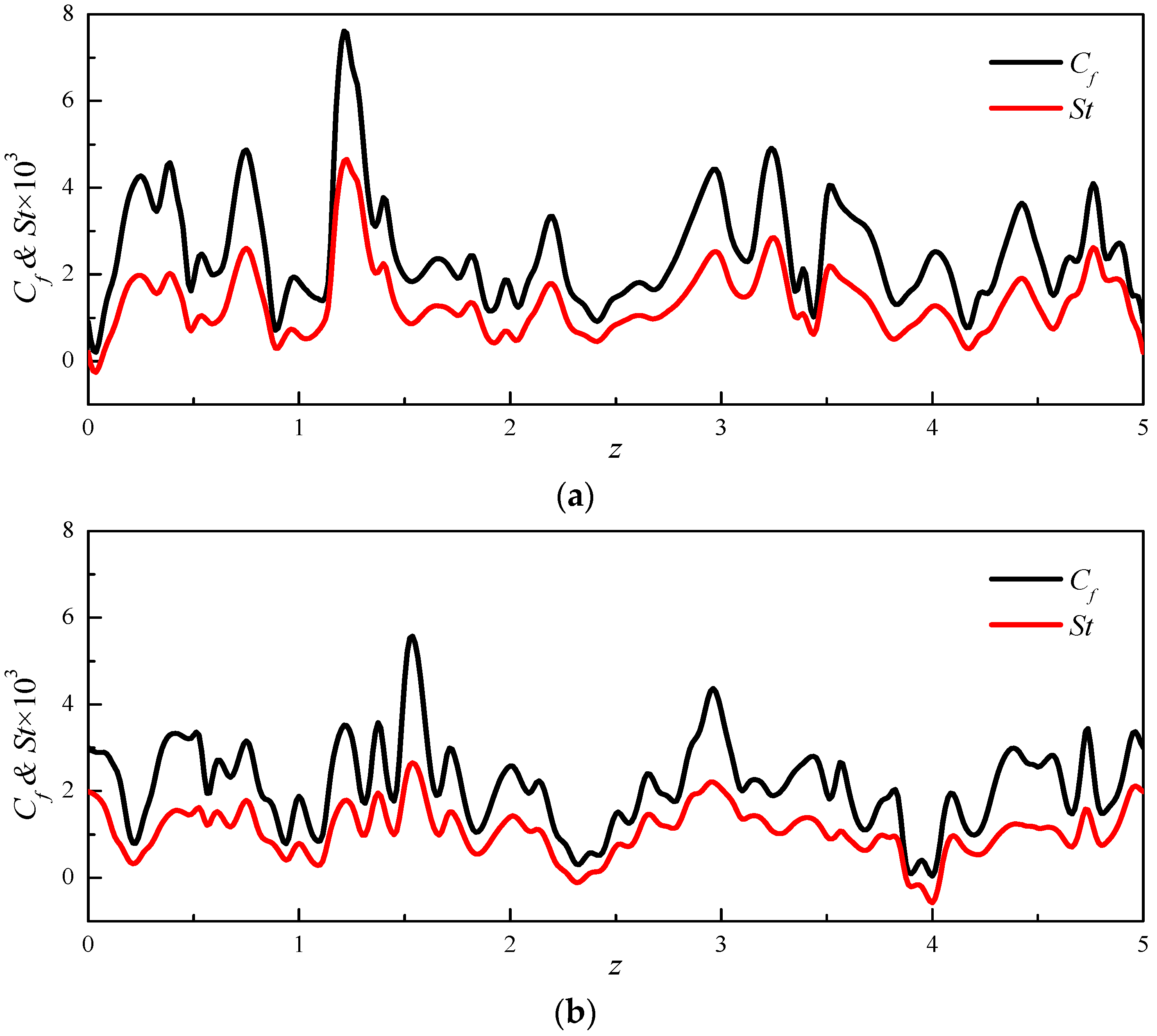
3.5. Reynolds Analogy

To validate the consistent mechanism of momentum and heat transports concluded above, both the Reynolds analogy between skin friction and Stanton number and the strong Reynolds analogy are conducted.

The instantaneous spanwise distributions of skin friction coefficient $C_f$ and Stanton number $St$, defined as:

$$C_f=\frac{{\mu }_w}{Re}\frac{{\partial u/\partial y|}_w}{0.5{\rho }_{ref}{u}_{ref}^2},$$

(20)

and

$$St={{\mu }_w\frac{\partial T}{\partial y}|}_w\frac{1}{{\rho }_{ref}{u}_{ref}\left(T_t-T_w\right)PrRe},$$

(21)

at the section of x = 40.775 are plotted in Figure 17. $T_t$ in Equation (20) is the total temperature of the incoming flow defined as $T_t=T_0\left(1+\frac{1}{2}\left(\gamma -1\right)M^2\right)$.

As can be seen in Figure 17, $C_f$ and $St$ for all the cases have similar distributions, although their levels could be very different. Due to the strong heating effect of the Stokes layer in Case P150A20, the Stanton number is greatly increased even to about three times of that of the baseline case. It should be mentioned that, for wall oscillation with small amplitudes, the similarity between $C_f$ and $St$ can be preserved. However, for cases with large SWO amplitudes, the similarity could change with SWO phase. Figure 17c,d present distributions of $C_f$ and $St$ at two different time steps. We can see that the similarity is good for the first time step but not well preserved for the second one.

To further study the similarity, the correlation coefficient $C_{RA}$ is used to study the correlation between $C_f$ and $St$. $C_{RA}$ is defined as:

$$C_{RA}=\frac{{\langle \left(C_f-{\langle C_f\rangle }_s\right)\left(St-{\langle St\rangle }_s\right)\rangle }_s}{\sqrt{Va{r}_{C_f}Va{r}_{St}}},$$

(22)

in which ${\langle \rangle }_s$ denotes the spanwise averaged value of an instantaneous variable while $Va{r}_{C_f}$ and $Va{r}_{St}$ are the variances of spatial average.

The temporal evolution of $C_{RA}$ for Case P150A20 is presented in Figure 18. We can see that $C_{RA}$ is highly fluctuant between 0 and 1. The correlation between the peak of $C_{RA}$ and zero wall velocity can be identified; meanwhile, lower values of $C_{RA}$ correspond to the maximum wall velocity.

The statistic values of $\overline{C_f}$, $\overline{St}$ and $\overline{C_{RA}}$ are listed in

Table 3. Mean values of skin friction, Stanton number and their correlation.

Case	$\overline{{\mathit{C}}_{\mathit{f}}}\mathbf{\times }{\mathbf{10}}^{\mathbf{3}}$	$\overline{\mathit{S}\mathit{t}}\mathbf{\times }{\mathbf{10}}^{\mathbf{3}}$	$\overline{{\mathit{C}}_{\mathit{R}\mathit{A}}}$
0	2.55	1.36	95%
P150A3	2.14	1.08	93%
P150A20	1.48	5.92	56%

. We can see that Case P150A3 gets reductions of both $C_f$ and $St$, although the reduction levels are quite limited. In Case P150A20, a great reduction of $C_f$ is observed, but a massive increase of $St$ is also induced.The correlation $\overline{C_{RA}}$ has a high value close to 100% for both Case 0 and P150A3, which means the Reynolds analogy is well preserved for SWO with small amplitude. However, due to the temporal fluctuation of $C_{RA}$, $\overline{C_{RA}}$ of Case P150A20 is reduced to 56%, indicating the weakening of Reynolds analogy, which may aggravate with the increase of wall oscillation amplitude. Nevertheless, the clear positive correlation over 50% can be confirmed for all cases, which means the preservation of Reynolds analogy for the studied cases.

The strong Reynolds analogy is conducted by analyzing the cross correlation between streamwise velocity fluctuations and temperature fluctuations $R\left(T^{″},u^{″}\right)$ defined as

$$R\left(T^{″},u^{″}\right)=\frac{\langle T^{″}{u}^{″}\rangle }{\sqrt{\langle T^{″}{T}^{″}\rangle \langle u^{″}{u}^{″}\rangle }}.$$

(23)

Profiles of $R\left(T^{″},u^{″}\right)$ at the section of x = 40.775 are plotted in Figure 19.

$R\left(T^{″},u^{″}\right)$ has a uniform negative value of −0.7 in the most part of the boundary layer, indicating a strong negative correlation between $T^{″}$ and $u^{″}$ in the boundary layer as represented in Figure 16. $R\left(T^{″},u^{″}\right)$ becomes positive near the wall due to the positive temperature gradient in the near-wall region. $R\left(T^{″},u^{″}\right)$ reaches zero at the location of the mean temperature peak, where the mean temperature gradient is equal to zero.

Comparing the three cases, the effects of SWO on $R\left(T^{″},u^{″}\right)$ are very limited. Only a slight reduction of $R\left(T^{″},u^{″}\right)$ close to the wall for Case P150A20 can be observed. Therefore, the strong Reynolds analogy is well preserved for cases with SWO.

4. Conclusions

The Mach = 2.9 turbulent boundary layer with SWO is investigated using DNS. The DNS data are analyzed to study the effect of SWO on temperature field and turbulent heat transport, especially the relation with velocity field and momentum transport. The following conclusions are reached:

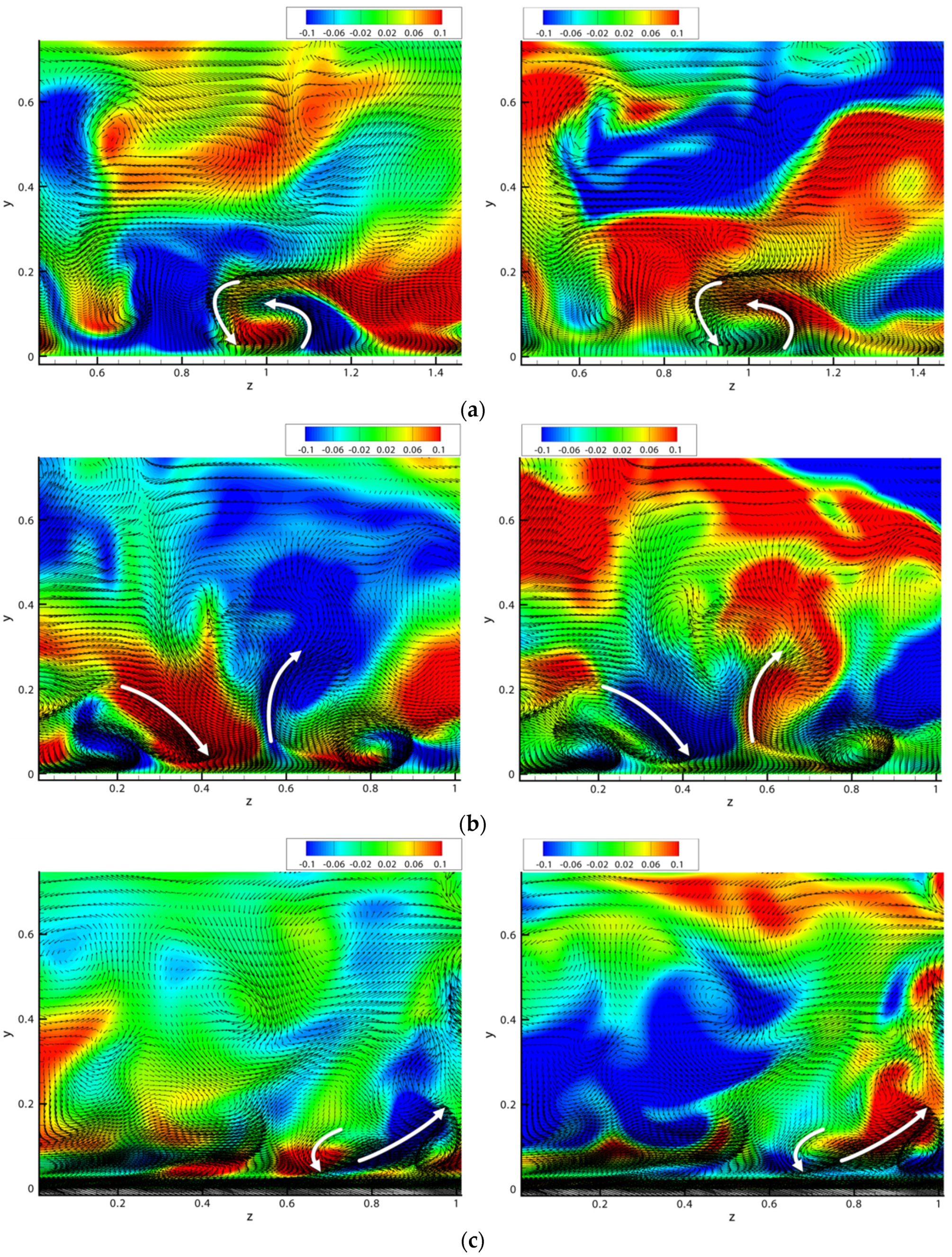
• The turbulent coherent structures are suppressed by SWO, especially for cases with large SWO amplitude. The drag is reduced to a similar level with that of the incompressible flow, indicating a limited influence of the compressibility on the drag reduction. The absolute values of Reynolds stresses are reduced by SWO, while the reduction might be not so obvious when the local friction velocity is used as the reference.
• WHF, mean temperature profile and temperature fluctuation statistics are modified by SWO differently with drag, mean velocity profile and velocity fluctuation statistics. Due to the heating effect of the spanwise Stokes layer induced by SWO, WHF is largely increased for most cases. The reduction of WHF is possible to be realized only with carefully optimized SWO parameters.
• The analysis of heat transport reveals that the underline heat transport mechanism of turbulence is consistent with turbulent momentum transport for both controlled and uncontrolled cases. They are both dominated by the sweep and ejection motions of streamwise vortices in the boundary layer.
• Consequently, the correlation and corresponding relations of temperature field and velocity field are well preserved. Both the Reynolds analogy and strong Reynolds analogy hold.
• Therefore, it is possible to apply turbulent drag reduction technologies to suppressing WHF by reducing turbulent heat transport in the supersonic turbulent boundary layer.

References

1. Korkegi, R.H. Survey of viscous interaction associated with high Mach number flight. AIAA J. 1971, 9, 771–784. [Google Scholar] [CrossRef]
2. Aso, S.; Kumamoto, Y.; Kondo, N.; Nakamura, Y.; Katayama, M.; Kurosaki, R. Aerodynamic heating with boundary layer transition and heat protection with mass addition on blunt body in hypersonic flows. In Proceedings of the 23rd Fluid Dynamics, Plasmadynamics, and Lasers Conference, Orlando, FL, USA, 6–9 July 1993.
3. Li, F.C.; Kawaguchi, Y. Investigation on the characteristics of turbulence transport for momentum and heat in a drag-reducing surfactant solution flow. Phys. Fluids 2004, 16, 3281–3295. [Google Scholar] [CrossRef]
4. Stalio, E.; Nobile, E. Direct numerical simulation of heat transfer over riblets. Int. J. Heat Fluid Flow 2003, 24, 356–371. [Google Scholar] [CrossRef]
5. Fang, J.; Lu, L. Large eddy simulation of compressible turbulent channel flow with active spanwise wall fluctuations. Mod. Phys. Lett. 2010, B2, 1457–1460. [Google Scholar] [CrossRef]
6. Jung, W.J.; Mangiavacchi, N.; Akhavan, R. Suppression of turbulence in wall-bounded flows by high-frequency spanwise oscillations. Phys. Fluids A 1992, 4, 1605–1607. [Google Scholar] [CrossRef]
7. Laadhari, F.; Skandaji, L.; Morel, R. Turbulence reduction in a boundary layer by a local spanwise oscillation surface. Phys. Fluids 1994, 6, 3218–3220. [Google Scholar] [CrossRef]
8. Baron, A.; Quadrio, M. Turbulent drag reduction by spanwise wall oscillations. Appl. Sci. Res. 1995, 55, 311–326. [Google Scholar] [CrossRef]
9. Choi, K.S.; DeBisschop, J.R.; Clayton, B.R. Turbulent boundary layer control by means of spanwise-wall oscillation. AIAA J. 1998, 36, 1157–1163. [Google Scholar] [CrossRef]
10. Choi, K.S.; Clayton, B.R. The mechanism of turbulent drag reduction with wall oscillation. Int. J. Heat Fluid Flow 2001, 22, 1–9. [Google Scholar] [CrossRef]
11. Quadrio, M. Drag reduction in turbulent boundary layers by in-plane wall motion. Phil. Trans. R. Soc. A 2011, 369, 1428–1442. [Google Scholar] [CrossRef] [PubMed]
12. Trujillo, S.M.; Bogard, D.G.; Ball, K.S. Turbulent boundary layer drag reduction using an oscillating wall. In Proceedings of the 4th AIAA Shear Flow Control Conference, Snowmass Village, CO, USA, 25 June 1997.
13. Ricco, P.; Wu, S. On the effects of lateral wall oscillations on a turbulent boundary layer. Exp. Therm. Fluid Sci. 2004, 29, 41–52. [Google Scholar] [CrossRef]
14. Skote, M. Temporal and spatial transients in turbulent boundary layer flow over an oscillating wall. Int. J. Heat Fluid Flow 2013, 38, 1–12. [Google Scholar] [CrossRef]
15. Quadrio, M.; Ricco, P. Critical assessment of turbulent drag reduction through spanwise wall oscillations. J. Fluid Mech. 2004, 521, 251–271. [Google Scholar] [CrossRef] [Green Version]
16. Ricco, P.; Quadrio, M. Wall-oscillation conditions for drag reduction in turbulent channel flow. Int. J. Heat Fluid Flow 2008, 29, 891–902. [Google Scholar] [CrossRef]
17. Hasegawa, Y.; Quadrio, M.; Frohnapfel, B. Numerical simulation of turbulent duct flows with constant power input. J. Fluid Mech. 2014, 750, 191–209. [Google Scholar] [CrossRef] [Green Version]
18. Fang, J.; Lu, L.; Shao, L. Large eddy simulation of compressible turbulent channel flow with spanwise wall oscillation. Sci. China Ser. G 2009, 52, 1233–1243. [Google Scholar] [CrossRef]
19. Fang, J.; Lu, L.; Shao, L. Heat transport mechanisms of low Mach number turbulent channel flow with spanwise wall oscillation. Acta Mech. Sin. 2010, 26, 391–399. [Google Scholar] [CrossRef]
20. Lele, S.K. Compact finite difference schemes with spectral-like resolution. J. Comput. Phys. 1992, 103, 16–42. [Google Scholar] [CrossRef]
21. Sandham, N.D.; Li, Q.; Yee, H.C. Entropy splitting for high–order numerical simulation of compressible turbulence. J. Comput. Phys. 2002, 178, 307–322. [Google Scholar] [CrossRef]
22. Gaitonde, D.V.; Visbal, M.R. Pade-type higher-order boundary filtersfor the Navier-Stokes Equations. AIAA J. 2000, 38, 2103–2112. [Google Scholar] [CrossRef]
23. Gottlieb, S.; Shu, C.W. Total variation diminishing Runge-Kutta schemes. Math. Comput. 1998, 67, 73–85. [Google Scholar] [CrossRef]
24. Yudhistira, I.; Skote, M. Direct numerical simulation of a turbulent boundary layer over an oscillating wall. J. Turbulence 2011, 12, 1–17. [Google Scholar] [CrossRef]
25. Sagaut, P. Theoretical Background: Large-Eddy Simulation, Large-Eddy Simulation for Acoustics, 1st ed.; Cambridge University Press: Cambridge, UK, 2007; pp. 89–127. [Google Scholar]
26. Touber, E.; Sandham, N.D. Large-eddy simulation of low-frequency unsteadiness in a turbulent shock-induced separation bubble. Theor. Comput. Fluid Dyn. 2009, 23, 79–107. [Google Scholar] [CrossRef]
27. Kim, J.W.; Lee, D.J. Generalized characteristic boundary conditions for computational aeroacoustics. AIAA J. 2000, 38, 2040–2049. [Google Scholar] [CrossRef]
28. Kim, J.W.; Lee, D.J. Generalized characteristic boundary conditions for computational aeroacoustics, part 2. AIAA J. 2004, 41, 47–55. [Google Scholar] [CrossRef]
29. Gatti, D.; Quadrio, M. Performance losses of drag-reducing spanwise forcing at moderate values of the Reynolds number. Phys. Fluids 2013, 25, 125109. [Google Scholar] [CrossRef]
30. Murlis, J.; Tsai, H.M.; Bradshaw, P. The structure of turbulent boundary layers at low Reynolds numbers. J. Fluid Mech. 1982, 122, 12–56. [Google Scholar] [CrossRef]
31. Erm, L.P.; Joubert, P.N. Low Reynolds number turbulent boundary layers. J. Fluid Mech. 1991, 230, 1–44. [Google Scholar] [CrossRef]
32. Martin, M.P. Direct numerical simulation of hypersonic turbulent boundary layers Part 1. Initialization and comparison with experiments. J. Fluid Mech. 2007, 570, 347–364. [Google Scholar] [CrossRef]
33. Lagha, M.; Kim, J.; Eldredge, J.D.; Zhong, X. A numerical study of compressible turbulent boundary layers. Phys. Fluids 2011, 23, 015106. [Google Scholar] [CrossRef]
34. Guarini, S.E.; Moser, R.D.; Shariff, K.; Wray, A. Direct numerical simulation of a supersonic turbulent boundary layer at Mach 2.5. J. Fluid Mech. 2000, 414, 1–33. [Google Scholar] [CrossRef]
35. Fang, J.; Yao, Y.; Zheltovodov, A.A.; Li, Z.; Lu, L. Direct numerical simulation of supersonic turbulent flows around a tandem expansion-compression corner. Phys. Fluids 2000, 27, 125104. [Google Scholar] [CrossRef]
36. Purtell, L.P.; Klebanoff, P.S.; Buckley, F.T. Turbulent boundary layer at low Reynolds number. Phys. Fluids 1981, 24, 802. [Google Scholar] [CrossRef]
37. Spalart, P.R. Direct numerical simulation of a turbulent boundary layer up to Reθ = 1410. J. Fluid Mech. 1988, 187, 61–98. [Google Scholar] [CrossRef]
38. Wu, X.; Moin, P. Direct numerical simulation of turbulence in a nominally zero-pressure-gradient flat-plate boundary layer. J. Fluid Mech. 2009, 630, 5–41. [Google Scholar] [CrossRef]
39. Pirozzoli, S.; Bernardini, M.; Grasso, F. Direct numerical simulation of transonic shock/boundary layer interaction under conditions of incipient separation. J. Fluid Mech. 2010, 657, 361–393. [Google Scholar] [CrossRef]
40. Duan, L.; Beekman, I.; Martin, M.P. Direct numerical simulation of hypersonic turbulent boundary layers. Part 2. Effect of wall temperature. J. Fluid Mech. 2010, 655, 419–445. [Google Scholar] [CrossRef]
41. Zhou, J.; Adrian, R.J.; Balachandar, S.; Kendall, T.M. Mechanisms for generating coherent packets of hairpin vortices in channel flow. J. Fluid Mech. 1999, 387, 353–396. [Google Scholar] [CrossRef]
42. Iuso, G.; Cicca, G.M.D.; Onoratob, M.; Spazzini, P.G.; Malvano, R. Velocity streak structure modifications induced by flow manipulation. Phys. Fluids 2003, 15, 2602–2612. [Google Scholar] [CrossRef]
43. Touber, E.; Leschziner, M.A. Near-wall streak modification by spanwise oscillatory wall motion and drag-reduction mechanisms. J. Fluid Mech. 2012, 693, 150–200. [Google Scholar] [CrossRef]
44. Quadrio, M.; Ricco, P. The laminar generalized stokes layer and turbulent drag reduction. J. Fluid Mech. 2011, 667, 135–157. [Google Scholar] [CrossRef]
45. Skote, M. Turbulent boundary layer flow subject to streamwise oscillation of spanwise wall-velocity. Phys. Fluids 2011, 23, 081703. [Google Scholar] [CrossRef]
46. Kim, J.; Moin, P.; Moser, R. Turbulence statistics in fully developed channel flow at low Reynolds number. J. Fluid Mech. 1987, 177, 133–166. [Google Scholar] [CrossRef]
47. Jiménez, J.; Pinelli, A. The autonomous cycle of near wall turbulence. J. Fluid Mech. 1999, 389, 335–359. [Google Scholar] [CrossRef]
48. Jiménez, J. Near-wall turbulence. Phys. Fluids 2013, 25, 101302. [Google Scholar] [CrossRef]
Figure 1. Sketch of the boundary layer flow with spanwise wall oscillation (SWO).
Energies 09 00154 g001
Figure 2. Mean velocity profile in inner scaling at x = x s t a r t . The von Kármán constant is κ = 0.41.
Energies 09 00154 g002
Figure 3. Density-scaled root mean square (RMS) velocity fluctuation in outer scaling (a) and inner scaling (b) at x = x s t a r t .
Energies 09 00154 g003aEnergies 09 00154 g003b
Figure 4. Turbulent coherent structures visualized with iso-surface of λ c i (a) and velocity streak at y + = 10 (b).
Energies 09 00154 g004aEnergies 09 00154 g004b
Figure 5. The rates of the change of drag (DR) for Group 1 (a) and Group 2 (b).
Energies 09 00154 g005
Figure 6. The rates of the change of wall heat flux (HR) for Group 1 (a) and Group 2 (b).
Energies 09 00154 g006
Figure 7. Temporal evolutions of wall heat flux. Data from DNS are spanwise averaged results.
Energies 09 00154 g007
Figure 8. Corrected HR for Group 1 (a) and Group 2 (b).
Energies 09 00154 g008
Figure 9. Averaged WHF of laminar Stokes solution and Case P150A20.
Energies 09 00154 g009
Figure 10. Mean velocity profile in outer scaling (a) and inner scaling (b) at x = 40.775. The local wall variables are used to normalize y + and u V D + in (b).
Energies 09 00154 g010
Figure 11. Mean temperature profile at x = 40.775.
Energies 09 00154 g011
Figure 12. Turbulent velocity fluctuation intensities at x = 40.775: (a) Streamwise velocity intensity; (b) wall-normal velocity intensity; and (c) spanwise velocity intensity.
Energies 09 00154 g012aEnergies 09 00154 g012b
Figure 13. Turbulent temperature fluctuation intensity (a) and zoomed in near wall region (b) at x = 40.775.
Energies 09 00154 g013
Figure 14. Profiles of Reynolds shear stress (a) and normal turbulent heat flux (b) at x = 40.775. The near-wall region in (b) is zoomed in (c).
Energies 09 00154 g014aEnergies 09 00154 g014b
Figure 15. Cross correlations of momentum transport R ( u , v ) (a) and heat transport R ( T , v ) (b) at x = 40.775.
Energies 09 00154 g015
Figure 16. Distributions of velocity vector ( w , v ) , streamwise velocity fluctuation u (left) and temperature fluctuation T (right) at x = 40.775 in instantaneous flow field: (a) Case 0; (b) Case P150A3; and (c) Case P150A20. The white arrows represent the local sweep and ejection motions.
Energies 09 00154 g016
Figure 17. Spanwise distributions of C f and S t at x = 40.775 in instantaneous flow fields: (a) Case 0; (b) Case P150A3; (c) Case P150A20 at t = 767.4; and (d) Case P150A20 at t = 781.8.
Energies 09 00154 g017aEnergies 09 00154 g017b
Figure 18. Temporal evolution of C R A for Case P150A20.
Energies 09 00154 g018
Figure 19. Cross correlations of T and u at x = 40.775.
Energies 09 00154 g019