Optimization of Train Operation in Multiple Interstations with Multi-Population Genetic Algorithm

Abstract

Subway systems consume a large amount of energy each year. How to reduce the energy consumption of subway systems has already become an issue of concern in recent years. This paper proposes an energy-efficient approach to reduce the traction energy by optimizing the train operation for multiple interstations. Both the trip time and driving strategy are considered in the proposed optimization approach. Firstly, a bi-level programming model of multiple interstations is developed for the energy-efficient train operation problem, which is then converted into an integrated model to calculate the driving strategy for multiple interstations. Additionally, the multi-population genetic algorithm (MPGA) is used to solve the problem, followed by calculating the energy-efficient trip times. Finally, the paper presents some examples based on the operation data of the Beijing Changping subway line. The simulation results show that the proposed approach presents a better energy-efficient performance than that with only optimizing the driving strategy for a single interstation.

1. Introduction

With the rapid development of railway transportation, the energy consumption problem of the railway transportation industry is becoming prominent. Many people give much focus to energy-efficient strategies. Train traction energy consumption accounts for the largest proportion in subway systems, which is closely related to the train operation. Hence, reducing the traction energy by optimizing the train operation becomes more important.

Many studies have been focusing on the energy-efficient operation of railway trains. The earliest research is based on the assumption that there are no speed limits and ramps in the lines. Ishikawa [1] studied the optimal control model with constant traction efficiency. Erofeyev [2] solved the model by using a dynamic programming method. For applying the theory into practice, many studies take gradients, speed limit and variable traction efficiency into consideration. For example, Milroy [3] and Asnis et al. [4] put forward a model with constant slope in the lines, then calculated the optimal control sequence with the minimum energy consumption. Golovitcher [5,6] studied the problem with variable gradients to find the general rules for optimizing the control sequence. Howlett et al. [7] studied an analytical method for the problem with steep slopes in the route. Khmelnitsky [8] proved that the optimal train driving strategy consists of maximum acceleration, cruising, coasting and maximum braking. Li et al. [9] studied the energy-efficient operation with an energy constraint, while the trip time was considered to be related to the energy consumption.

As for integrated models optimizing the timetable and driving, Ding et al. [10] developed a two-level hierarchical model to minimize the energy consumption for a train running on an uneven rail with the specific trip time based on the characteristics of train movement and the control rules of the locomotive. Ning et al. [11] proposed an integrated control method to optimize train headway by adjusting the train arrival time at stations; the speed profiles for each train were also obtained. Ghoseiri et al. [12] formulated a multi-objective optimization model for the passenger train-scheduling problem, in which single and multiple tracks and multiple platforms with different train capacities are considered. Cucala et al. [13] considered uncertainty in delays, then designed a model for energy-efficient driving and timetables, in which the railway operator and administrator requirements are also included. Kwan and Chang [14] studied a dual objective problem including energy consumption and passenger dissatisfaction in a medium-sized mass rapid transit system; a heuristic-based evolutionary algorithm was used to solved it. On the other hand, many studies focus on the efficient driving of the train. Albrecht et al. [15] proved that the optimal switching points are uniquely defined for each steep section, and the global optimal strategy is also unique. Carvajal et al. [16] proposed an optimization algorithm to obtain the minimum energy consumption and the Pareto optimal curve for CBTC (communication-based train control). Bocharnikov et al. [17] considered both the tractive energy consumption and the utilization of regenerative energy to obtain the minimum energy consumption for a single train, and then, a multi-train simulation was performed to optimize the net energy consumption. Acikbas and Soylemez [18] obtained the optimal coasting point using artificial neural networks and genetic algorithms. Chuang et al. [19] used an artificial neural network to optimize the coasting speed of the train to minimize both the energy consumption and passenger traveling time.

In recent years, various algorithms have been successfully applied to the studies of the energy-efficient operation of railway trains. Wong and Ho [20,21,22,23] searched the coasting position by search algorithms, such as the golden section method, gradient search and the genetic algorithm, to optimize the driving strategy and formulated a tri-level model for the train control system. Kim and Chien [24] searched for the optimal operation by a simulated annealing algorithm while considering speed limit and track alignment. Lu et al. [25] developed a speed profile searching model that considered equipment characteristics, speed limits and gradients; dynamic programming, the genetic algorithm and the colony optimization algorithm were applied to search the optimal speed profile. Gong et al. [26] proposed an energy-efficient operation methodology for metro system; a genetic algorithm was used to modify the dwell time of each stop to obtain the most optimal energy-efficient timetable. Tuyttens et al. [27] studied a real-time traffic control strategy to obtain the speed profiles for every train on the route based on the genetic algorithm. Fu [28] calculated the switch position of the energy-efficient driving strategy, which considered the specific driving regime sequence. Liu and Golovitcher [29] solved the energy-efficient operation strategy of the train also by using the maximum principle and finally obtained the switch point by using a numerical algorithm. Rémy [30] minimized the trip time and energy consumption by using the genetic algorithm. Ke et al. [31,32,33] designed the energy-efficient speed sequence of the block sections and calculated the optimal operation speed by using the ACO(ant colony optimization) algorithm. Yu [34] further optimized the algorithm of this problem and further improved the calculation speed. Dominguez et al. [35] optimized the speed profile using the genetic algorithm; regenerative energy was taken into account. Rodrigo et al. [36] also focused on the use of regeneration energy; a Lagrangian multipliers method was proposed to solve the problem by optimizing the speed profile. Yang et al. [37] designed a genetic algorithm to maximize the use of regeneration energy by optimizing the timetable. Table 1 is the summary list of the studies.

Table 1. Summary list of the studies.

Publication	Research Contents	Algorithm
Wong and Ho [20,21,22,23]	Coasting control	Golden section method
		Gradient search
		Genetic algorithm
Kim and Chien [24]	Speed Profile	Simulated annealing algorithm
Lu et al. [25]	Speed profile	Dynamic programming, genetic
		algorithm and colony
		optimization algorithm
Gong et al. [26]	Energy-efficient timetable	Genetic algorithm
Tuyttens et al. [27]	Speed profiles	Genetic algorithm
Fu [28] Liu	Switch position for driving regime	Genetic algorithm
and Golovitcher [29]		Numerical algorithm
Rémy [30]	Minimized the energy consumption	Genetic algorithm
	and trip time
Ke et al. [31,32,33], Yu [34]	Energy-efficient speed	ACO algorithm
	sequence of the block sections
Dominguez et al. [35]	Speed profile + regenerative energy	Genetic algorithm [24]
Rodrigo et al. [36]	Timetable + regenerative energy	Lagrangian multipliers method [25]
Yang et al. [37]		Genetic algorithm
Our paper	Trip time + switch position	Multi-population genetic algorithm
	for driving regime

Table 1. Summary list of the studies.

Publication	Research Contents	Algorithm
Wong and Ho [20,21,22,23]	Coasting control	Golden section method
		Gradient search
		Genetic algorithm
Kim and Chien [24]	Speed Profile	Simulated annealing algorithm
Lu et al. [25]	Speed profile	Dynamic programming, genetic
		algorithm and colony
		optimization algorithm
Gong et al. [26]	Energy-efficient timetable	Genetic algorithm
Tuyttens et al. [27]	Speed profiles	Genetic algorithm
Fu [28] Liu	Switch position for driving regime	Genetic algorithm
and Golovitcher [29]		Numerical algorithm
Rémy [30]	Minimized the energy consumption	Genetic algorithm
	and trip time
Ke et al. [31,32,33], Yu [34]	Energy-efficient speed	ACO algorithm
	sequence of the block sections
Dominguez et al. [35]	Speed profile + regenerative energy	Genetic algorithm [24]
Rodrigo et al. [36]	Timetable + regenerative energy	Lagrangian multipliers method [25]
Yang et al. [37]		Genetic algorithm
Our paper	Trip time + switch position	Multi-population genetic algorithm
	for driving regime

Previous studies only optimize the driving strategy with the fixed trip time in the timetable, which ignores the influence of trip time on the energy consumption. Actually, the trip time and driving strategy are closely related to each other and can make a difference in energy savings. Firstly, the trip time that is scheduled by the timetable is an important constraint for the driving strategy, and there is an optimal driving strategy, costing the least energy consumption. Secondly, the trip time of multiple intervals consists of the minimum trip time and reserve time; the distribution of reserve time will influence the total energy consumption (Figure 1).

Figure 1. Different timetables for multiple interstations.

Figure 1. Different timetables for multiple interstations.

In addition, the amount of energy consumption determined by the driving strategy can be the basis of optimizing the trip times [38]. Therefore, to reduce the energy consumption of the subway system, both the driving strategy and trip times, as well as the relationship between them, should be considered. The aim of this paper is to obtain an integrated solution to the energy-efficient train operation problem. Considering the constraints of speed limits and gradients of the real subway line, an optimization model is formulated for multiple interstations based on the energy-efficient driving strategy for interstations, then the speed profile and trip times are calculated based on the multi-population genetic algorithm.

2. Model Formulation

The aim of this paper is to minimize the total energy consumption of multiple interstations. A bi-level programming model is developed for the energy-efficient problem, where the high level aims to optimize the trip time and the low level is to find the energy-efficient driving strategy. Then, an integrated model is concluded to solve the driving strategy for multiple interstations, which can obtain the energy-efficient trip time, as well.

In order to facilitate the understanding of this paper, the assumptions, the parameters and the variables are introduced firstly.

2.1. Assumptions

The train is considered as a particle; the length of the train is not considered.

2.2. Decision Variables

$T_{\text{interstation}i}$: trip time for the i-th interstation.

$C_{i,j}$: driving regime for the i-th section in the j-th interstation.

2.3. Intermediate Variables

v: speed of the train.

$V_i$: final speed for the i-th section.

$v_{ij}$: final speed for the j-th subsection in the i-th section.

$a_{ij}$: acceleration for the j-th subsection in the i-th section.

$a^{\mathrm{T}}$: equivalent acceleration for the traction force.

$F_{ij}$: traction force for the j-th subsection in the i-th section.

$F_{{\text{br}}_{ij}}$: basic resistance for the j-th subsection in the i-th section.

$F_{\mathrm{gr}}$: gradient resistance force.

$F_{\mathrm{cr}}$: curve resistance force.

$E_{\mathrm{s}}$: the optimal energy consumption.

$E_i$: energy consumption for the i-th section per unit mass.

$e_{ij}$: energy consumption for the j-th subsection in the i-th section per unit mass.

$T_{\mathrm{s}}$: the optimal trip time.

$T_i$: trip time for the i-th section.

$t_{ij}$: trip time for the j-th subsection in the i-th section.

$T_{\text{interstation}i}^{\min }$: minimum trip time for the i-th interstation.

$T_{\text{interstation}i}^{\max }$: maximum trip time for the i-th interstation.

2.4. Parameters

k: number of interstations.

p: number of sections in an interstation.

m: number of subsections in a section.

w: number of driving regimes in an interstation.

T${}_{\mathrm{p}}$: the practical trip time.

S${}_i$: trip distance for the i-th section.

$S_{\text{interstation}i}$: trip distance for the i-th interstation.

M${}_i$: mass of the train for the i-th interstation.

d: trip distance for each subsection.

$v_{\text{limit}}$: speed limits.

E${}_{\mathrm{p}}$: the practical energy consumption.

α: penalty coefficient of time in the objective function.

β: penalty coefficient of speed in the objective function.

$T_{\text{dwell}i}$: dwell time for the i-th interstation.

2.5. Model

In general, the train’s energy-efficient operation in subway systems contains two levels. At the high level, a timetable is designed, which regulates the trip time and the dwell time for trains. The low level calculates the energy-efficient speed profile for each interstation with the trip time and the dwell time given by the high level. In addition, the dwell times are not included in the model, and that total trip time does not include the dwell times. The dwell time for each station remains unchanged when optimizing the timetable.

The high level can be describe as Equation (1a), and (1b). The object in Equation (1a) is to solve the minimum energy consumption of the entire route, and the decision variable in Equation (1a), and (1b) is $T_{\text{interstation}i}$. Equation (1b) is the constraints and boundary conditions, in which the first equation denotes the constraints on the energy consumption; the last two equations denote the constraints on the trip time.

$$\begin{array}{c}\hfill min{E}_s=\sum _{i=1}^k{M}_{i}E\left(T_{\mathrm{intersation} i}\right)\end{array}$$

(1a)

$$\begin{array}{c}\hfill s.t.\left\{\begin{array}{c}E\left(T_{\mathrm{interstation}i}\right)={\displaystyle \sum _{i=1}^p}{E}_i\hfill \\ T_p=T_s={\displaystyle \sum _{i=1}^k}{T}_{\mathrm{interstation}i}\hfill \\ T_{\mathrm{interstation}i}^{min}\le T_{\mathrm{interstation}i}\le T_{\mathrm{interstation}i}^{max}\hfill \end{array}\right.\end{array}$$

(1b)

The low level can be describe as Equation (2a), and (2b). The object Function (2a) is to solve the minimum energy consumption of a given interstation with a given trip time T${}_{\mathrm{interstation}i}$. The decision variable in Equation (2a), and (2b) is the driving regime sequence C${}_i$. Equation (2b) is the constraints and boundary conditions, in which the first two equations denote the constraints on the energy consumption and train speed. The last two inequalities denote the constraints about the comfort of passengers.

$$\begin{array}{c}\hfill minE\left(T_{\mathrm{interstation}i}\right)=\sum _{i=1}^p{E}_i\left(C_i\right)\end{array}$$

(2a)

$$\begin{array}{c}\hfill s.t.\left\{\begin{array}{c}{E}_i\left(C_i\right)={\displaystyle \sum _{j=1}^m}{a}_{(i,j)}^{T}d\hfill \\ v\left(0\right)=0,v\left(T_{\mathrm{interstation}i}\right)=0,0\le v_i\le v_{lim\mathrm{it}}\hfill \\ w\le w_{limit},\left|C_{i+1}-C_i\right|\le 1\hfill \end{array}\right.\end{array}$$

(2b)

The bi-level optimization model can be summarized as Equation (3a), and (3b):

$$\begin{array}{c}\hfill min{E}_s\left(C_{i,j}\right)\end{array}$$

(3a)

$$\begin{array}{c}\hfill s.t.\left\{\begin{array}{c}{E}_{\mathrm{s}}\left(C_{i,j}\right)={\displaystyle \sum _{j=1}^k}{M}_j({\displaystyle \sum _{i=1}^p}{E}_i\left(C_{i,j}\right))\hfill \\ E_i={\displaystyle \sum _{j=1}^m}{a}_{(i,j)}^{T}d\hfill \\ T_p=T_{\mathrm{s}}={\displaystyle \sum _{i=1}^k}{T}_{\mathrm{interstation}i}\hfill \\ T_{\mathrm{interstation}i}^{min}\le T_{\mathrm{interstation}i}\le T_{\mathrm{int}erstationi}^{max}\hfill \\ v\left(0\right)=0,v\left(T_{\mathrm{interstation}i}\right)=0,0\le v_i\le v_{lim\mathrm{it}}\hfill \\ w\le w_{limit},\left|C_{i+1,j}-C_{i,j}\right|\le 1\hfill \end{array}\right.\end{array}$$

(3b)

In the model above, the object Function (3a) is to solve the minimum energy consumption of the entire route, and the decision variable in Equation (3a), and (3b) is the driving regime sequence C${}_{i,j}$. Equation (2b) is the constraints and boundary conditions; the first two equations denote the constraints on the energy consumption; the third and fourth equations denote the constraints on the trip time; and the fifth equation denotes the constraints on the train speed. The last two inequalities denote the constraints about the comfort of passengers.

3. Solution

Standard genetic algorithm (SGA) has many advantages in optimization, but premature convergence usually happens in SGA when solving multi-peak value problems, which means the optimal solution is easily trapped in local optima, and it cannot find the global optimal solution. In order to overcome the premature convergence, the authors calculate the driving regime sequence based on the multi-population genetic algorithm (MPGA). The basic idea of MPGA is to use a plurality of sub-populations instead of a single population in the algorithm. Each sub-population selects crossover and mutation independently based on SGA. Superior individuals can migrate between sub-populations after preset generations in order to improve the average fitness value of sub-populations and to ensure the genetic diversity. Figure 2 shows the structure of MPGA. There are three sub-populations in Figure 2; each of them operates based on SGA. The dotted lines show the migration track of superior individuals between sub-populations. Part of the best fitness individuals from these three sub-populations finally constitute the quintessence population of MPGA.

Figure 2. Multi-population genetic algorithm structure diagram. Standard genetic algorithm: SGA.

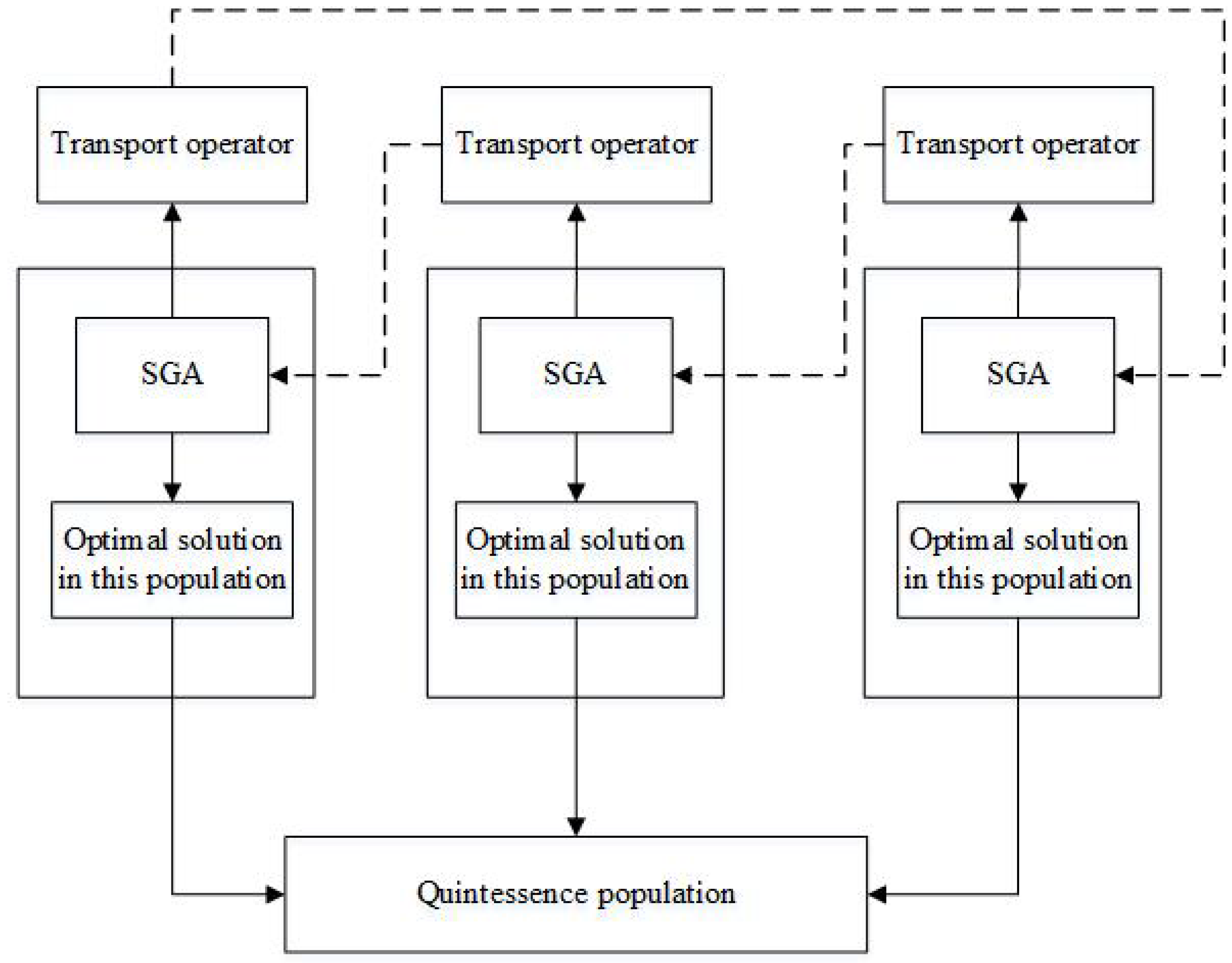
Figure 2. Multi-population genetic algorithm structure diagram. Standard genetic algorithm: SGA.

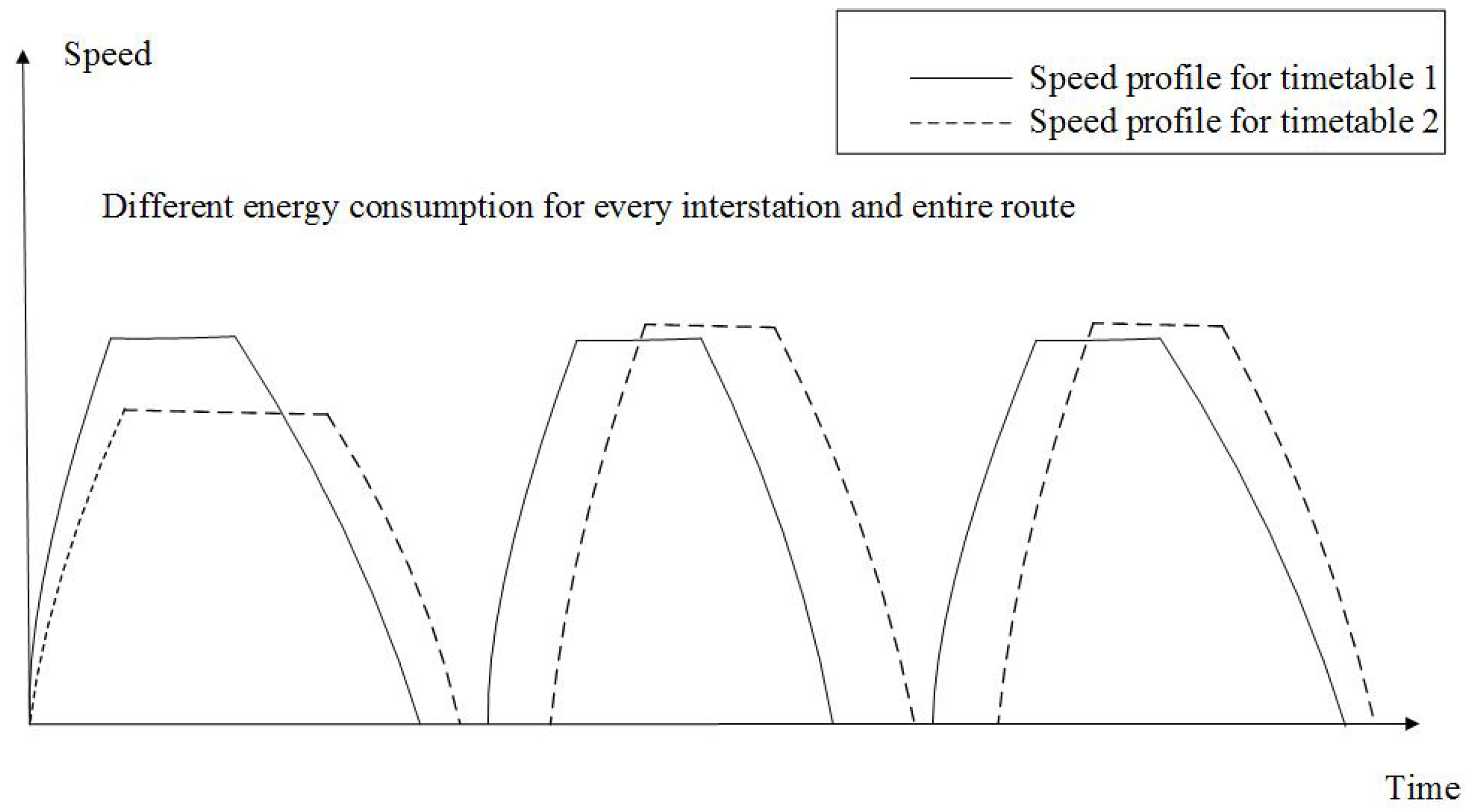
3.1. Energy-Efficient Operation Strategy

The trip time and energy consumption of multiple interstations is determined by the order and switching positions of the driving regime, which include maximum acceleration, coasting and maximum braking. There are many feasible speed profiles that satisfy the constraints on trip time and trip distance; each of them determines a driving strategy and the corresponding energy consumption. The energy-efficient optimization is to find a driving strategy that costs the minimum energy consumption on the condition that the total trip time is relatively constant.

Previous research [39] shows that the energy-efficient driving strategy in the interstation includes acceleration, coasting and braking. Thomas [40] explained the optimal phases as follows.

• Maximum acceleration and braking: The slower a train accelerates or brakes, the more time it needs to come to a standstill. To obtain the same trip time with a lower acceleration or braking rate, the train should accelerate to a higher speed, which consumes more energy. Therefore, the maximum acceleration and braking must be the most energy efficient.
• Coasting: During coasting, when no traction force and braking force are applied, the train only rolls forward and consumes no energy. Thus, the earlier coasting can start, the more energy can be saved.

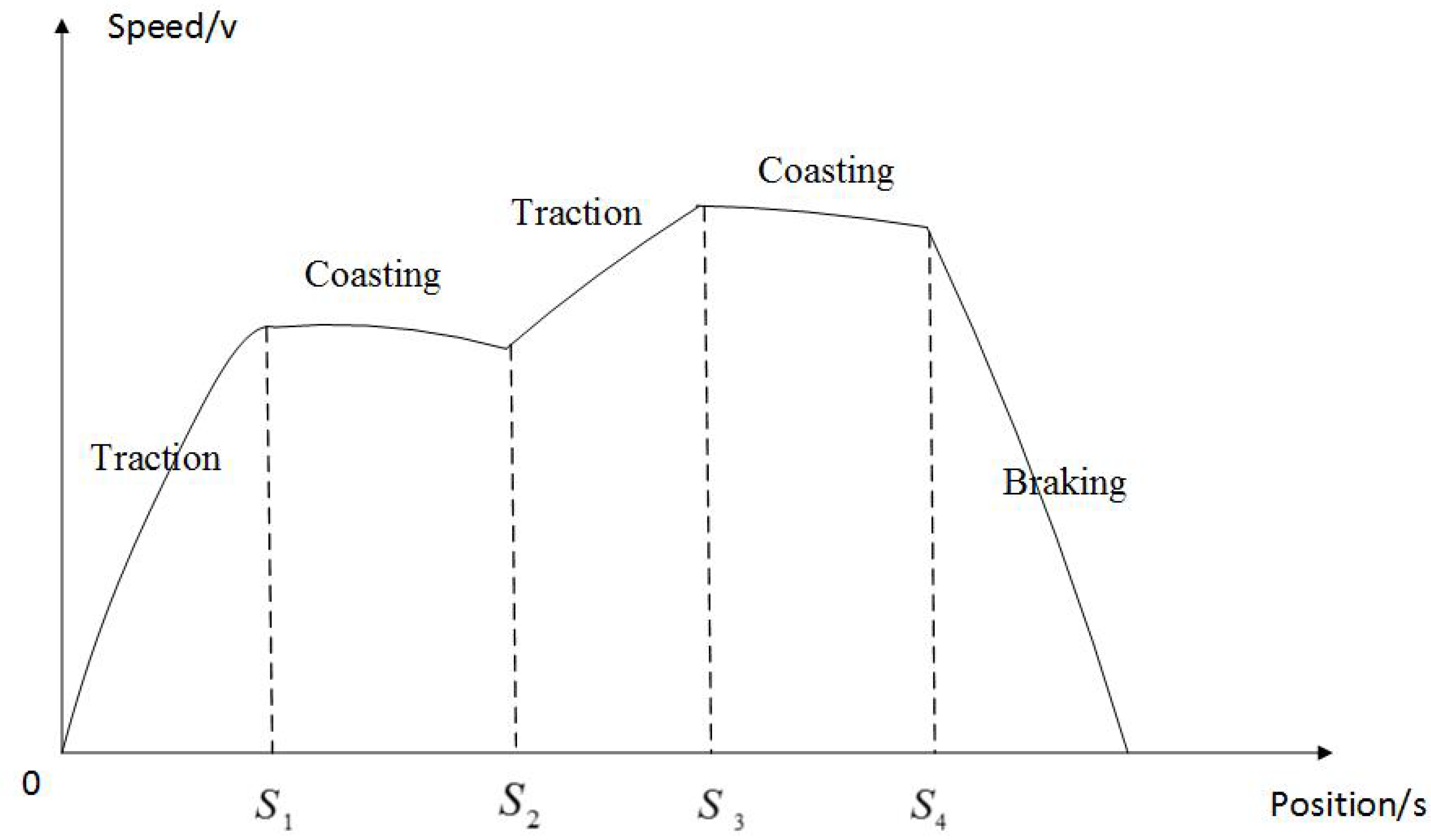
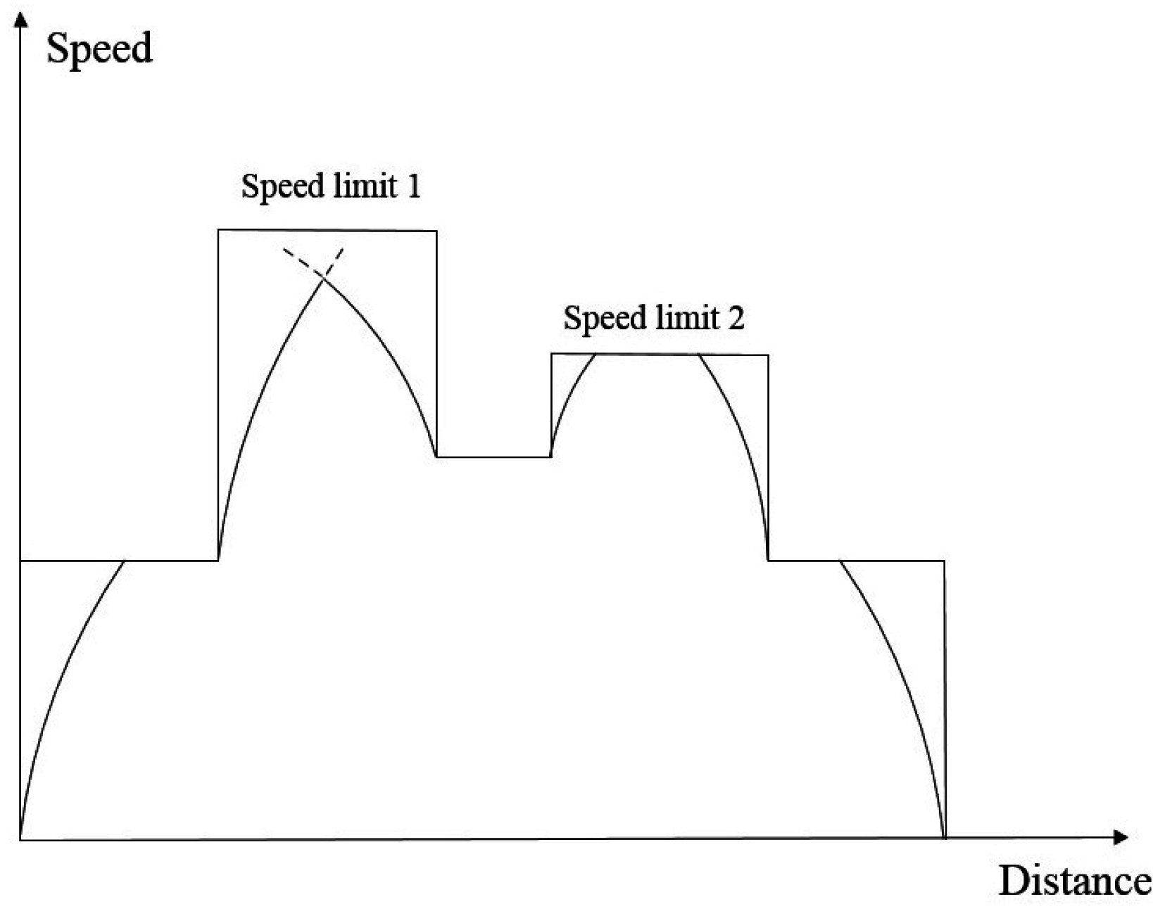
As shown in Figure 3, S${}_1$, S${}_3$ denotes the switching position from acceleration to coasting, S${}_2$ denotes the switching position from coasting to acceleration and S${}_4$ denotes the switching position from coasting to braking.

Figure 3. Optimal driving strategy for interstations.

Figure 3. Optimal driving strategy for interstations.

It is assumed that the total trip distance of multiple interstations is L; then, L is divided into n sections, and the trip distance of each section can be expressed as $S_i=(s_1,s_2,\cdots ,s_n)$. Each section is short enough to allow only one driving regime, so there are n driving regimes, which could be regarded as a driving regime sequence $C_i=(c_1,c_2,\cdots ,c_n)$ for the entire route. Here, the corresponding relations between the driving regimes are listed in Table 2.

Table 2. Definition for driving regimes.

Number	Driving Regimes	Value
1	Traction	1
2	Coasting	2
3	Braking	3

Table 2. Definition for driving regimes.

Number	Driving Regimes	Value
1	Traction	1
2	Coasting	2
3	Braking	3

The driving regime sequence C${}_i$ must follow the constraint as follows:

• The first driving regime for an interstation must be ”1” (Traction), the last one for an interstation must be ”3” (Braking).
• Considering the comfort of passengers, traction and braking are not allowed to directly switch to each other. The change of the driving regimes must follow the rules listed in Table 3 [41] in order to limit the jerk, in which ”√” donates the change is allowed, ”×” donates the change is forbidden.
• Also considering the comfort of passengers, the driving regime change times for an interstation must follow the constraints in Table 4. according to the operation experience. Specially, the maximum change time in Table 4. is empirical value and the value will be sensibly adjusted for interstations which contain steep slopes, low speed limits and other special conditions.

Table 3. Rules for the change of the driving regimes.

Driving Regime	Traction	Coasting	Braking
Traction	√	√	×
Coasting	√	√	√
Braking	×	√	√

Table 3. Rules for the change of the driving regimes.

Driving Regime	Traction	Coasting	Braking
Traction	√	√	×
Coasting	√	√	√
Braking	×	√	√

Table 4. Constraints for the driving regimes’ change times.

Number	Distance (m)	Maximum Change Times
1	0–1000	3
2	1000–3000	5
3	3000–5000	7

Table 4. Constraints for the driving regimes’ change times.

Number	Distance (m)	Maximum Change Times
1	0–1000	3
2	1000–3000	5
3	3000–5000	7

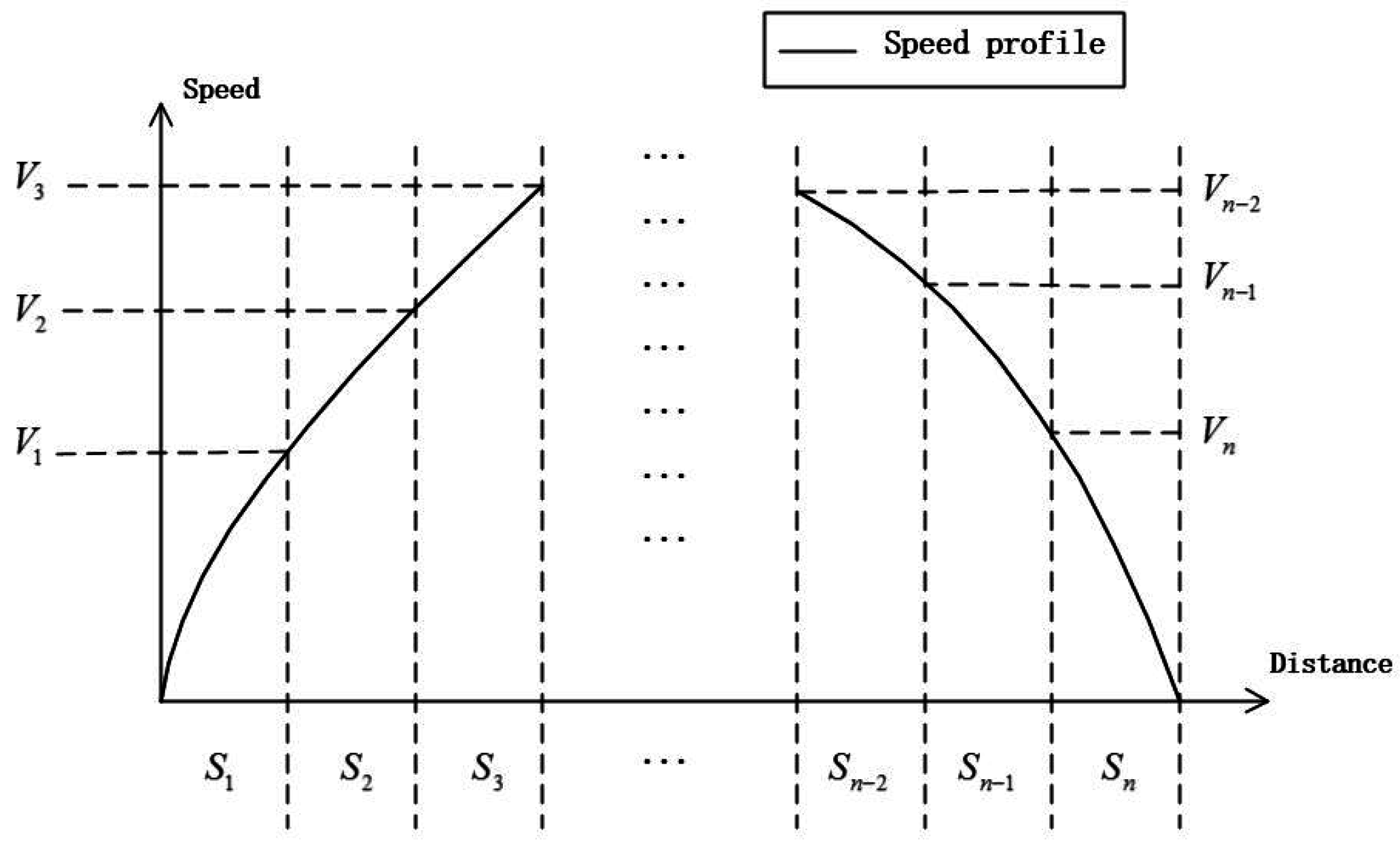
As shown in Figure 4, the final speed of each section V${}_i$, trip time T${}_i$ and energy consumption E${}_i$ can be calculated according to the driving regime C${}_i$, the trip distance S${}_i$ and the initial speed V${}_{i-1}$. The final speed of the section “i” will be iterated as the initial speed of the section “i + 1”. Then, the total trip time and energy consumption of the interstation can be obtained when the driving strategy is determined for all sections. Both the energy consumption reduction and the computing time of the algorithm will be influenced by the value of S${}_i$. On the one hand, a smaller value of S${}_i$ may leads to a larger energy consumption reduction, because the driving regime could be more changeable; on the other hand, a smaller value of S${}_i$ means more variables in the algorithm, which will lead to longer computing. In this paper, S${}_i$ is 50 m in order to keep the balance of the two sides.

Figure 4. Calculation model.

Figure 4. Calculation model.

In order to ensure the accuracy of the results, a section should be divided into small subsections for calculation. It is assumed that there are m subsections in the i-th section; the trip distance of each subsection is d. The final speed v${}_{(i,j)}$, trip time t${}_{(i,j)}$ and energy consumption e${}_{(i,j)}$ of each subsection can be calculated according to the initial speed v${}_{(i,j-1)}$, trip distance d and driving regime C${}_i$. In addition, with the consideration of the number of commuters, the mass of the train for each interstation M${}_i$ varies with different interstations. In this paper, the authors define M${}_i$ as a random variable obeying a normal distribution. Thus, the probability distribution of M${}_i$ can be expressed as Equation (4), in which μ can be defined as Equation (5). In Equation 5, M${}_{\max }$ denotes the full load mass of the train, and M${}_{\min }$ denotes the empty mass of the train.

$$\begin{array}{c}\hfill f\left(M_i\right)=\frac{1}{\sqrt{2}\mathsf{\pi }}exp(-\frac{(M_i-\mathsf{\mu })}{2})\end{array}$$

(4)

$$\begin{array}{c}\hfill \mathsf{\mu }=(M_{max}+M_{min})/2\end{array}$$

(5)

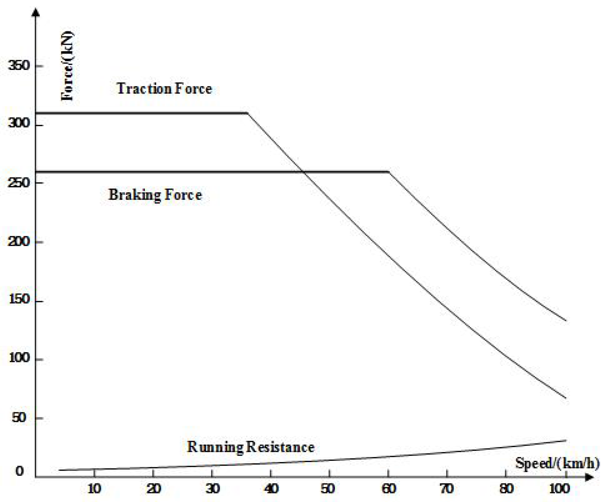
Here, t${}_{(i,j)}$, e${}_{(i,j)}$ of each subsection are firstly calculated. Here, in this paper, the acceleration for the traction process is considered to be varied with the traction force. The acceleration for the braking process is considered to be a constant.

When the driving regime in the i-th section is acceleration, traction force is used to speed up the train and overcome resistance (Equation (6)):

$$\begin{array}{c}\hfill \left\{\begin{array}{c}{a}_{(i,j)}^T=a_{(i,j)}+({\mathsf{\omega }}_{(i,j)}^b+{\mathsf{\omega }}_{(i,j)}^g+{\mathsf{\omega }}_{(i,j)}^c)g\hfill \\ v_{(i,j)}=\sqrt{{v_{(i,j-1)}}^2+2a_{(i,j)}d}\hfill \\ t_{(i,j)}=\left|v_{(i,j)}-v_{(i,j-1)}/\phantom{v_{(i,j)}-v_{(i,j-1)}{a}_{(i,j)}}{a}_{(i,j)}\right|\hfill \\ e_{(i,j)}=a_{(i,j)}^{T}d\hfill \end{array}\right.\end{array}$$

(6)

Then, the final speed $V_i$, trip time $T_i$ and energy consumption $E_i$ of the i-th section can be calculated. The final speed $V_i$ of the section is the final speed $v_{(i,j)}$ of the last subsection. The trip time of the section is the sum of subsections (Equation (7)).

$$\begin{array}{c}\hfill \left\{\begin{array}{c}{V}_i=v_{(i,n)}\hfill \\ T_i={\displaystyle \sum _{j=1}^m}{t}_{(i,j)}\hfill \\ E_i={\displaystyle \sum _{j=1}^m}{e}_{(i,j)}\hfill \end{array}\right.\end{array}$$

(7)

Similarly, when the driving regime in the i-th section is coasting or braking, the final speed $V_i$, trip time $T_i$ and energy consumption $E_i$ of the i-th section can be calculated according to the above method.

When the driving regime in the i-th section is coasting, the acceleration varies with the basic resistance and gradient resistance. The train is without traction, so the $E_i$ is zero (Equations (8) and (9)).

$$\begin{array}{c}\hfill \left\{\begin{array}{c}{a}_{(i,j)}=-({\mathsf{\omega }}_{(i,j)}^b+{\mathsf{\omega }}_{(i,j)}^g+{\mathsf{\omega }}_{(i,j)}^c)g\hfill \\ v_{(i,j)}=\sqrt{{v_{(i,j-1)}}^2+2a_{(i,j)}d}\hfill \\ t_{(i,j)}=\left|v_{(i,j)}-v_{(i,j-1)}/\phantom{v_{(i,j)}-v_{(i,j-1)}{a}_{(i,j)}}{a}_{(i,j)}\right|\hfill \\ e_{(i,j)}=0\hfill \end{array}\right.\end{array}$$

(8)

$$\begin{array}{c}\hfill \left\{\begin{array}{c}{V}_i=v_{(i,m)}\hfill \\ T_i={\displaystyle \sum _{j=1}^m}{t}_{(i,j)}\hfill \\ E_i=0\hfill \end{array}\right.\end{array}$$

(9)

When the driving regime in the i-th section is braking (Equations (10) and (11)):

$$\begin{array}{c}\hfill \left\{\begin{array}{c}{v}_{(i,j)}=\sqrt{{v_{(i,j-1)}}^2+2a_{(i,j)}d}\hfill \\ t_{(i,j)}=\left|v_{(i,j)}-v_{(i,j-1)}/\phantom{v_{(i,j)}-v_{(i,j-1)}{a}_{(i,j)}}{a}_{(i,j)}\right|\hfill \\ e_{(i,j)}=0\hfill \end{array}\right.\end{array}$$

(10)

$$\begin{array}{c}\hfill \left\{\begin{array}{c}{V}_i=v_{(i,m)}\hfill \\ T_i={\displaystyle \sum _{j=1}^m}{t}_{(i,j)}\hfill \\ E_i=0\hfill \end{array}\right.\end{array}$$

(11)

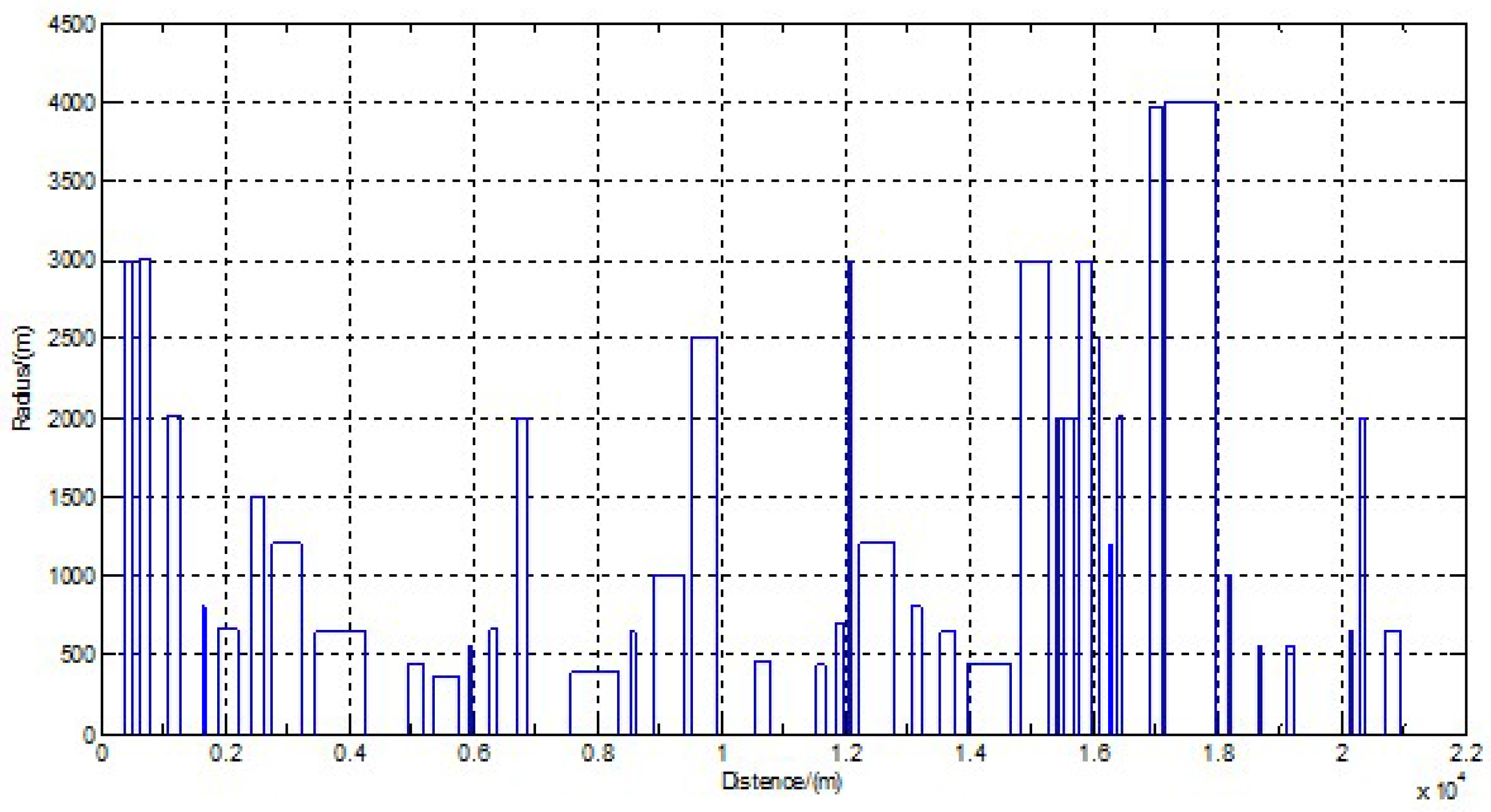
The basic resistance, gradient resistance and curve resistance are calculated as follows.

$$\begin{array}{c}\hfill {\mathsf{\omega }}_{\mathrm{b}}=a+bv+c{v}^2\end{array}$$

(12)

$$\begin{array}{c}\hfill {\mathsf{\omega }}_{\mathrm{g}}=i\end{array}$$

(13)

$$\begin{array}{c}\hfill {\mathsf{\omega }}_{\mathrm{c}}=\frac{600}{R}\end{array}$$

(14)

In Equation (12), a, b and c are empirical constants that vary with the vehicle type. In Equation (13), i denotes the value of the gradient. In Equation (14), R denotes the curve radius.

Therefore, there is a driving regime sequence $C_i=(c_1,c_2,\cdots ,c_n)$, which corresponds a trip time sequence $T_i=(T_1,T_2,\cdots ,T_n)$ and an energy consumption sequence $E_i=(E_1,E_2,\cdots ,E_n)$. Additionally, the corresponding total trip time is $T_s={\displaystyle \sum _{i=1}^n}{T}_i$. The total energy consumption is $E_s={\displaystyle \sum _{i=1}^n}{E}_i$. Therefore, the optimization problem can be formulated to obtain one driving regime sequence with minimum energy consumption on the condition that the total trip time is relatively constant.

There are constraints on trip time and constraints on speed in the optimization model mentioned above, so the optimization model for the MPGA is as follow:

$$\begin{array}{c}\hfill min\mathrm{obj}=E_{\mathrm{s}}+\left|T_{\mathrm{s}}-T_{\mathrm{t}}\right|·\mathsf{\alpha }+num·\mathsf{\beta }\end{array}$$

(15a)

$$\begin{array}{c}\hfill s.t.\left\{\begin{array}{c}{E}_{\mathrm{s}}\left(C_{i,j}\right)={\displaystyle \sum _{j=1}^k}{M}_j({\displaystyle \sum _{i=1}^p}{E}_i\left(C_{i,j}\right))\hfill \\ E_i={\displaystyle \sum _{j=1}^m}{a}_{(i,j)}^{T}d\hfill \\ T_{\mathrm{p}}=T_{\mathrm{s}}={\displaystyle \sum _{i=1}^k}{T}_{\mathrm{interstation}i}\hfill \\ T_{\mathrm{interstation}i}^{min}\le T_{\mathrm{interstation}i}\le T_{\mathrm{interstation}i}^{max}\hfill \\ v\left(0\right)=0,v\left(T_{\mathrm{int}\mathrm{erstation}i}\right)=0,0\le v_i\le v_{lim\mathrm{it}}\hfill \\ w\le w_{limit},\left|C_{i+1,j}-C_{i,j}\right|\le 1\hfill \end{array}\right.\end{array}$$

(15b)

In the model above, the first equation denotes the optimality criterion, in which num denotes the times that the speed does not satisfy the speed constraints in the speed profile, α denotes the penalty coefficient of time in the objective function and β denotes the penalty coefficient of speed in the objective function. α should be a very large number in order to ensure that the trip time is relatively constant. β is also very large because the speed profile must satisfy the speed constraints. In this way, individuals that do not satisfy the constraints will get large fitness values, and finally, they are eliminated. The following six equations denote the constraints on energy consumption, trip time, train speed and the constraints about the comfort of passengers.

3.2. Minimum Trip Time and Maximum Trip Time

According to Equation (1a), and (1b), the scheduled trip time for interstations must be longer than the minimum trip time and shorter than the maximum trip time. Here, a speed profile is drawn following the following steps, which must cost the minimum trip time.

• During the traction process, the speed profile is calculated with maximum traction force. The speed in the right ends of the speed limit sections is the maximum value that the train can get in the position, and the traction speed profile is drawn with maximum acceleration from the right end of each speed limit section. Therefore, the speed profile contains the maximum speed value the train can get in the corresponding position.
• During the braking process, the speed profile is calculated with maximum braking force. The speed in the left ends of the speed limit sections is the maximum value that the train can reach, and the braking speed profile is drawn with the maximum deceleration from the left end of each speed limit section. The train speed cannot exceed this braking speed profile, otherwise the train speed must exceed the speed limits at some position, which is not expected.
• The train speed cannot exceed the speed limit in any position according to the operation requirements.

Figure 5. Speed profile with minimum trip time.

Figure 5. Speed profile with minimum trip time.

Therefore, the speed profile above must cost the minimum trip time. According to the bidding documents of the Beijing Changping subway line signal system engineering special technical requirements, the maximum trip time can be calculated as Equation (16).

$$\begin{array}{c}\hfill T_{max}=k·T_{min}\end{array}$$

(16)

In this paper, the value of k is 1.2.

3.3. Algorithm

This problem is solved based on MPGA, and the process is as follows: Step 1: Initialize the initial data, including track limited speed, track slope value and train parameter value.

Step 2: Generate the initial population. Here, the authors use real code, describing the driving regime sequence by an individual $(c_1,c_2,\cdots ,c_N)$; the gene $C_i$ denotes a driving regime.

Step 3: Train operating calculations for calculating the total trip time $T_s$ and total energy consumption $E_s$ with the given driving regime sequence according to Equations (6)–(11).

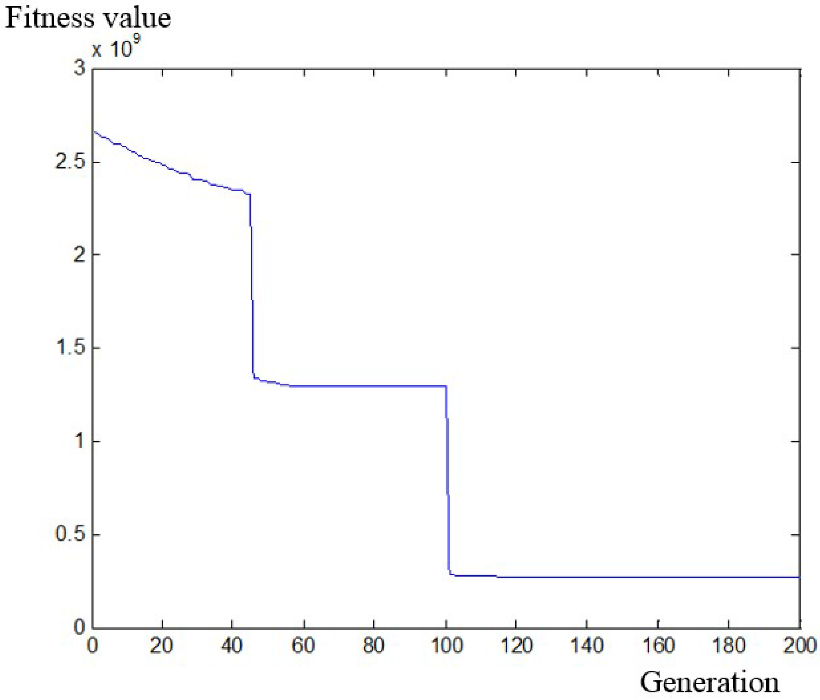
Step 4: Fitness calculation. The fitness function is the objective function of the optimization Model 3a,3b. $T_s$ and $E_s$ are inserted into the fitness function, and the fitness value of each individual is calculated.

Step 5: Generate new population. First, the selected operator is stochastic universal sampling; the crossover operator is discrete recombination; the mutation operator is real mutation. The insert strategy is to replace the worst individual in the father generation, so it is ensured that the best individual is always copiedinto the next generation. When satisfying the migration condition, a part of the best individuals migrate into adjacent subpopulations. Thus, a new generation consisting of new driving regime sequences is generated.

Step 6: Iteration number plus one. Make a judgment about whether the maximum iteration number is reached. If it is, skip to Step 7; if not, returnto Step 3.

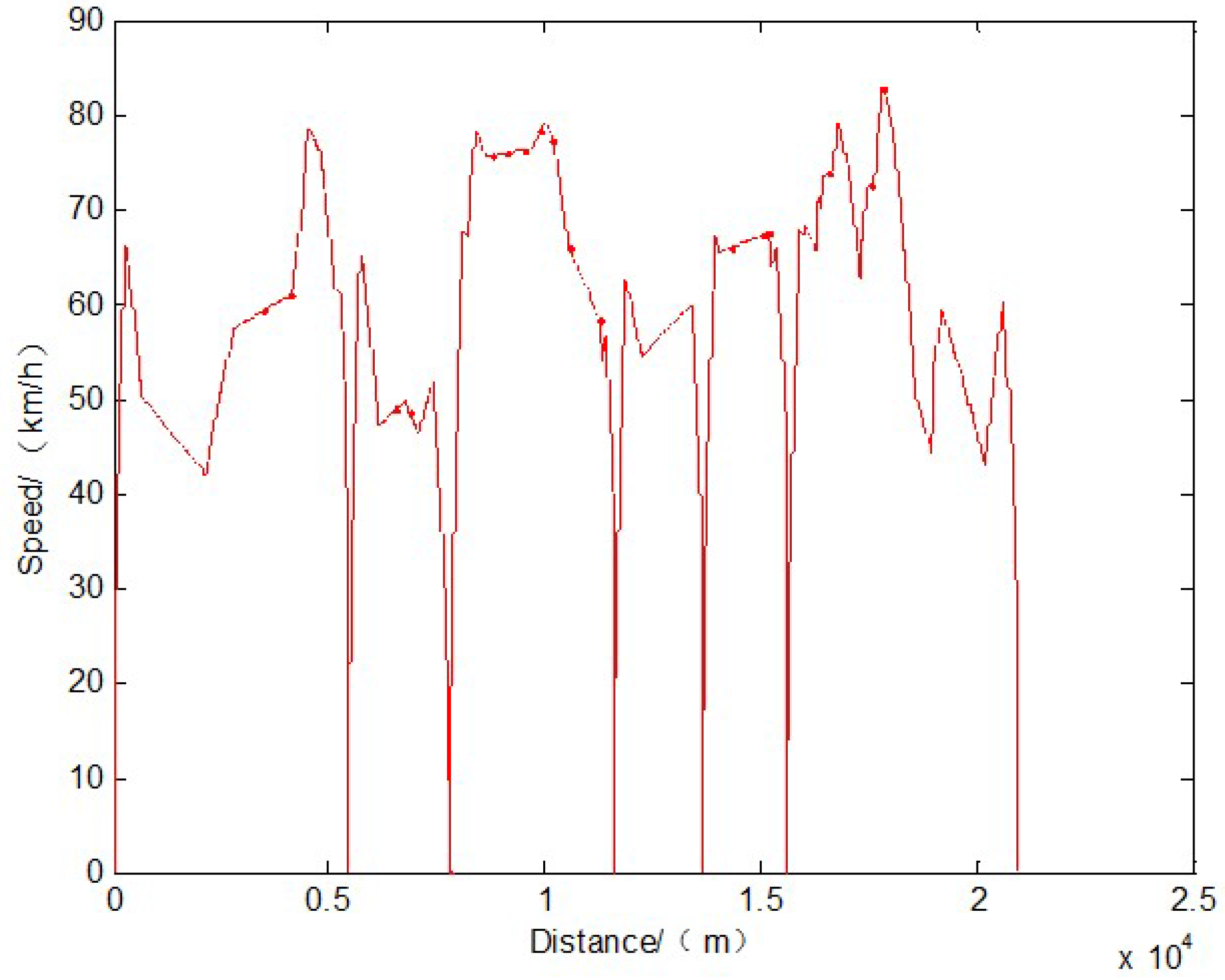
Step 7: Output the best driving regime sequence. $T_{\mathrm{s}}$ , $E_{\mathrm{s}}$ and the speed profile with the given driving regime sequence are calculated.

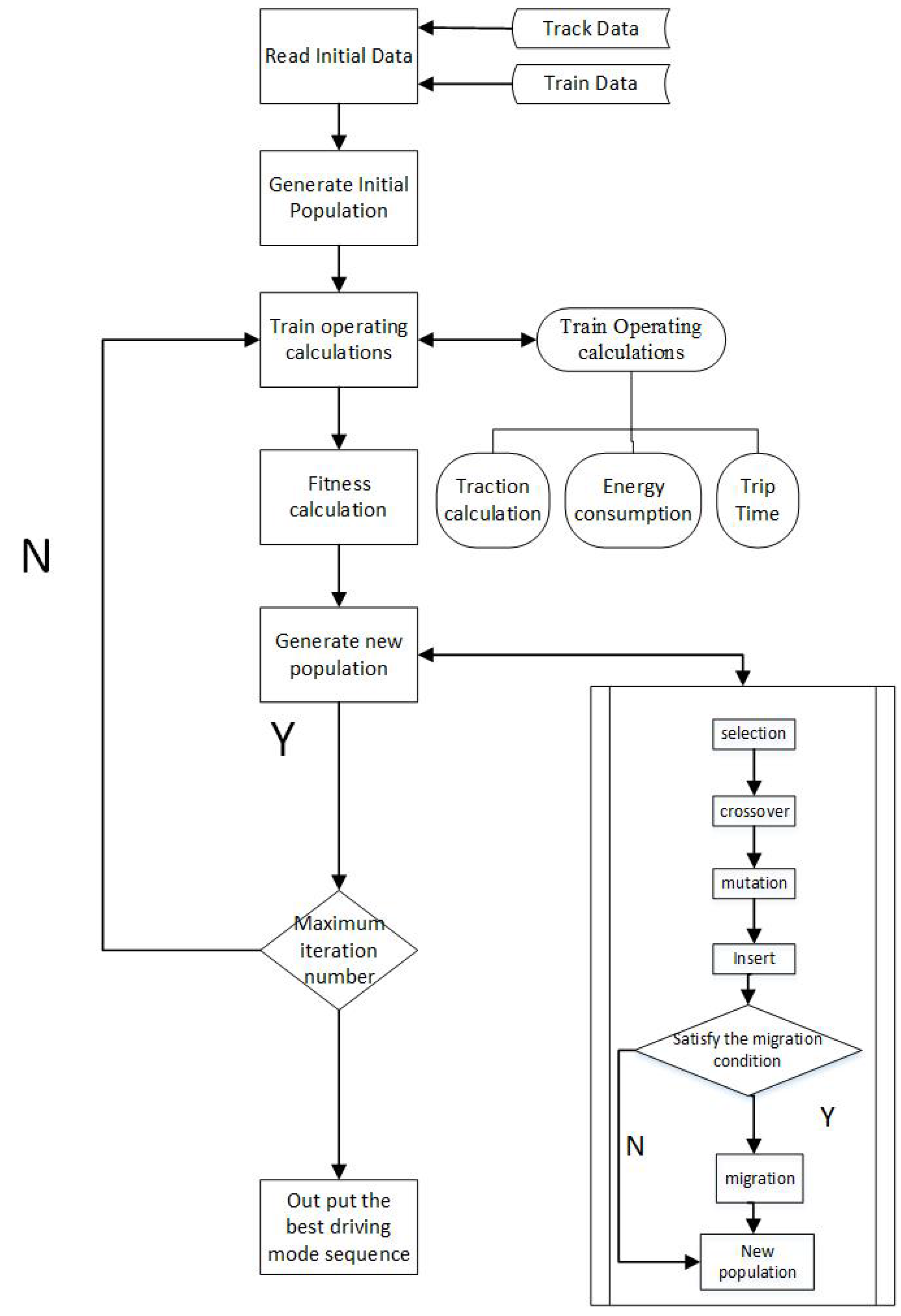
The algorithm flowchart is shown in Figure 6.

Figure 6. Algorithm flowchart for the multi-population genetic algorithm (MPGA).

Figure 6. Algorithm flowchart for the multi-population genetic algorithm (MPGA).

4. Case Study

To illustrate the effectiveness of the proposed model and algorithm, a case study based on the Beijing Changping subway line (Figure 7) is presented. The total Changping line covers a length of 21 km, consisting of seven stations and six interstations. The slope and curvature radius are variable and the maximum speed limit is 100 km/h. The operation requirements are listed in Table 5.

Figure 7. Beijing Changping subway line.

Figure 7. Beijing Changping subway line.

Table 5. Operation requirements of the Changping line.

Number	Interstation	Distance	T${}_{\mathbf{max}}$	T${}_{\mathbf{min}}$
		(m)	(s)	(s)
1	Xierqi-Shengmingkexueyuan	5441	370	308
2	Shengmingkexueyuan-Zhuxinzhuang	2368	191	159
3	Zhuxinzhuang-Gonghuacheng	3800	247	206
4	Gonghuacheng-Shahe	2025	148	123
5	Shahe-Shahegaojiaoyuan	1964	143	119
6	Shahegaojiaoyuan-Nanshao	5358	379	316

Table 5. Operation requirements of the Changping line.

Number	Interstation	Distance	T${}_{\mathbf{max}}$	T${}_{\mathbf{min}}$
		(m)	(s)	(s)
1	Xierqi-Shengmingkexueyuan	5441	370	308
2	Shengmingkexueyuan-Zhuxinzhuang	2368	191	159
3	Zhuxinzhuang-Gonghuacheng	3800	247	206
4	Gonghuacheng-Shahe	2025	148	123
5	Shahe-Shahegaojiaoyuan	1964	143	119
6	Shahegaojiaoyuan-Nanshao	5358	379	316

The slope data, curvature radius data and speed limit data in this case are listed in Figure 8 and Figure 9 and Table 6.

Figure 8. Slope data.

Figure 8. Slope data.

Figure 9. Curvature radius data.

Figure 9. Curvature radius data.

Table 6. Speed limit data.

Starting Position	End Position	Speed Limit	Starting Position	End Position	Speed Limit
(m)	(m)	(km/h)	(m)	(m)	(km/h)
0	4259	100	9901	10,548	86
4259	4960	86	10,548	10,758	100
4960	5196	100	10,758	11,528	84
5196	5356	76	11,528	11,671	100
5356	5740	100	11,671	11,816	73
5740	5933	91	11,816	13,730	100
5933	6872	100	13,730	13,962	74
6872	7550	79	13,962	20,956	100
7550	9901	100

Table 6. Speed limit data.

Starting Position	End Position	Speed Limit	Starting Position	End Position	Speed Limit
(m)	(m)	(km/h)	(m)	(m)	(km/h)
0	4259	100	9901	10,548	86
4259	4960	86	10,548	10,758	100
4960	5196	100	10,758	11,528	84
5196	5356	76	11,528	11,671	100
5356	5740	100	11,671	11,816	73
5740	5933	91	11,816	13,730	100
5933	6872	100	13,730	13,962	74
6872	7550	79	13,962	20,956	100
7550	9901	100

4.1. Train Traction Calculation

In the case study, the train is configured with three motor cars and three trailer cars; the characteristics of the train are listed in Table 7, in which W${}_m$ denotes the total mass of the motor cars, W${}_t$ denotes the total mass of trailer cars, v denotes the speed of the train, z denotes the number of service trains and i denotes the gradient value. In Table 7, the units of the force, mass and speed are kilonewtons, ton and kilometers per hour, respectively. The profile of train traction, braking force and basic resistance force is shown in Figure 10.

Table 7. Characteristics of the train.

Number	Parameters	Characteristics
1	Empty mass (T)	199
2	Full load mass (T)	311
3	Basic resistance (N)	$F_{\text{br}}\left(v\right)=\frac{(16.18+0.2422v)W_m}{1000}+\frac{(7.65+0.0275v)W_t}{1000}+\frac{[0.275+0.0765(z-1)]v^2}{1000}$
4	Tractive characteristic (kN)	$F\left(v\right)=\left\{\begin{array}{c}310,\text{if}v\le 36km/h\hfill \\ 310-3.67·(v-36),\text{if}v>36km/h\hfill \end{array}\right.$
5	Braking characteristic (kN)	$B\left(v\right)=\left\{\begin{array}{c}260,\text{if}v\le 60km/h\hfill \\ 260-3.25·(v-60),\text{if}v>60km/h\hfill \end{array}\right.$

Table 7. Characteristics of the train.

Number	Parameters	Characteristics
1	Empty mass (T)	199
2	Full load mass (T)	311
3	Basic resistance (N)	$F_{\text{br}}\left(v\right)=\frac{(16.18+0.2422v)W_m}{1000}+\frac{(7.65+0.0275v)W_t}{1000}+\frac{[0.275+0.0765(z-1)]v^2}{1000}$
4	Tractive characteristic (kN)	$F\left(v\right)=\left\{\begin{array}{c}310,\text{if}v\le 36km/h\hfill \\ 310-3.67·(v-36),\text{if}v>36km/h\hfill \end{array}\right.$
5	Braking characteristic (kN)	$B\left(v\right)=\left\{\begin{array}{c}260,\text{if}v\le 60km/h\hfill \\ 260-3.25·(v-60),\text{if}v>60km/h\hfill \end{array}\right.$

Figure 10. The profile of traction force, braking force and basic resistance force.

Figure 10. The profile of traction force, braking force and basic resistance force.

Figure 10 describes the traction force decreasing with the increase of train speed. This means that the acceleration is larger when the train speed is low, and the maximum traction force cannot support a large acceleration when the train travels at a high speed. Thus, in the traction process, the acceleration can be described as Equation (17). Condition 1 means that when the traction force is able to provide a large acceleration, the train acceleration is 0.8 m/s${}^2$ (0.8 m/s${}^2$ is the largest acceleration value according to the operation requirement). Condition 2 means when the traction force is too small to support the acceleration at 0.8 m/s${}^2$; the train will accelerate with the acceleration that the maximum traction force can provide:

$$\begin{array}{c}\hfill a=\left\{\begin{array}{c}0.8,\mathrm{condition}1\hfill \\ F_{\mathrm{T}}\left(v\right)-F_{\mathrm{br}}-F_{\mathrm{gr}}-F_{\mathrm{cr}}/\phantom{F_T\left(v\right)-F_{br}-F_{gr}-F_{cr}M}M,\mathrm{condition}2\hfill \end{array}\right.\end{array}$$

(17)

The authors simplify the acceleration as a constant in the braking process and fit the acceleration value based on the train operation data of the Changping line. The operation data of braking are listed in Table 8.

Table 8. Braking data of the Changping line.

Number	Time (s)	Speed	Distance	Acceleration
		(m/s)	(m)	(m/s${}^{\mathbf{2}}$)
1	358.8	18.32	5748	/
2	365	16.50	5857	−0.29
3	370	14.44	5934	−0.41
4	375	12.91	6002	−0.31
5	380	10.72	6061	−0.44
6	385	8.61	6109	−0.42
7	390	6.84	6148	−0.35
8	395	4.96	6182	−0.38
9	400	2.34	6196	−0.52
10	405.4	0	6202	−0.47

Table 8. Braking data of the Changping line.

Number	Time (s)	Speed	Distance	Acceleration
		(m/s)	(m)	(m/s${}^{\mathbf{2}}$)
1	358.8	18.32	5748	/
2	365	16.50	5857	−0.29
3	370	14.44	5934	−0.41
4	375	12.91	6002	−0.31
5	380	10.72	6061	−0.44
6	385	8.61	6109	−0.42
7	390	6.84	6148	−0.35
8	395	4.96	6182	−0.38
9	400	2.34	6196	−0.52
10	405.4	0	6202	−0.47

In the simulation case, the braking process is simplified as constant acceleration movements according to the practical operational data. Additionally, the acceleration can be calculated according to Equation (18). In this case, the average deceleration is − 0.39 m/s${}^2$.

$$\begin{array}{c}\hfill a=\frac{\Delta v}{\Delta t}\end{array}$$

(18)

4.2. Simulation Results

The simulation parameters of MPGA are shown in Table 9:

Table 9. Simulation parameters of MPGA.

Number	Simulation Parameters	Value
1	Maximum number of generations	200
2	Number of individuals	100
3	Number of sub-populations	8
4	Generation gap	0.8
5	Mutation rate	0.008
6	Insertion rate	0.9
7	Migration rate	0.2
8	Migration intervals	20
9	Time penalty coefficient (α)	10,000,000
10	Time penalty coefficient (β)	10,000,000

Table 9. Simulation parameters of MPGA.

Number	Simulation Parameters	Value
1	Maximum number of generations	200
2	Number of individuals	100
3	Number of sub-populations	8
4	Generation gap	0.8
5	Mutation rate	0.008
6	Insertion rate	0.9
7	Migration rate	0.2
8	Migration intervals	20
9	Time penalty coefficient (α)	10,000,000
10	Time penalty coefficient (β)	10,000,000

Figure 11 describes the fitness result of applying MPGA. The fitness value is decreasing from the first generation and soon keeps stable at the 117th generation, which reflects a good convergence.

Figure 11. Fitness value.

Figure 11. Fitness value.

The simulation results, which are shown in Table 10, show that the timetable is optimized (the high level), and the energy consumption reduction is 6.16%. In Table 10, T${}_{\mathrm{p}}$ denotes the practical trip time, T${}_{\mathrm{s}}$ denotes the optimal trip time, E${}_{\mathrm{p}}$ denotes the practical energy consumption and E${}_{\mathrm{s}}$ denotes the optimal energy consumption.

Table 10. Simulation results.

Interstation	Mass	T${}_{\mathbf{p}}$	T${}_{\mathbf{s}}$	E${}_{\mathbf{p}}$	E${}_{\mathbf{s}}$
	(t)	(s)	(s)	($\mathbf{kW}\mathbf{·}\mathbf{h}$)	($\mathbf{kW}\mathbf{·}\mathbf{h}$)
1	213	310	369	26.20	14.96
2	274	187	181	13.85	12.65
3	268	245	223	21.98	23.72
4	302	143	124	14.20	17.85
5	245	137	121	11.93	13.24
6	256	328	331	33.67	31.91
Total	-	1350	1349	121.83	114.33
Energy saving (%)	6.16%

Table 10. Simulation results.

Interstation	Mass	T${}_{\mathbf{p}}$	T${}_{\mathbf{s}}$	E${}_{\mathbf{p}}$	E${}_{\mathbf{s}}$
	(t)	(s)	(s)	($\mathbf{kW}\mathbf{·}\mathbf{h}$)	($\mathbf{kW}\mathbf{·}\mathbf{h}$)
1	213	310	369	26.20	14.96
2	274	187	181	13.85	12.65
3	268	245	223	21.98	23.72
4	302	143	124	14.20	17.85
5	245	137	121	11.93	13.24
6	256	328	331	33.67	31.91
Total	-	1350	1349	121.83	114.33
Energy saving (%)	6.16%

In addition, Figure 12 describes the optimization for the speed profile (the low level). The results shows that this method can reduce the energy consumption efficiently by regulating the trip time for multiple interstations on the condition that the total trip time is relatively constant.

Figure 12. The optimal speed profile.

Figure 12. The optimal speed profile.

5. Conclusions

This paper proposes an energy-efficient approach to reduce the traction energy by optimizing the train operation for multiple interstations. Both the trip time and driving strategy are considered in the proposed optimization approach. A bi-level programming model of multiple interstations is developed. The multi-population genetic algorithm is used to solve the problem.

Based on the operation data from the Beijing Changping subway line, a numerical example is given to prove that the proposed method can reduce the energy consumption of multiple interstations by 6.16%. Comparing this with the method that only optimizes the driving strategy with the fixed trip time in the timetable, both the trip time and driving strategy are considered, which leads to a better energy-efficient performance.