Metamodel for Efficient Estimation of Capacity-Fade Uncertainty in Li-Ion Batteries for Electric Vehicles

Abstract

This paper presents an efficient method for estimating capacity-fade uncertainty in lithium-ion batteries (LIBs) in order to integrate them into the battery-management system (BMS) of electric vehicles, which requires simple and inexpensive computation for successful application. The study uses the pseudo-two-dimensional (P2D) electrochemical model, which simulates the battery state by solving a system of coupled nonlinear partial differential equations (PDEs). The model parameters that are responsible for electrode degradation are identified and estimated, based on battery data obtained from the charge cycles. The Bayesian approach, with parameters estimated by probability distributions, is employed to account for uncertainties arising in the model and battery data. The Markov Chain Monte Carlo (MCMC) technique is used to draw samples from the distributions. The complex computations that solve a PDE system for each sample are avoided by employing a polynomial-based metamodel. As a result, the computational cost is reduced from 5.5 h to a few seconds, enabling the integration of the method into the vehicle BMS. Using this approach, the conservative bound of capacity fade can be determined for the vehicle in service, which represents the safety margin reflecting the uncertainty.

1. Introduction

Electric vehicles (EVs) or hybrid electric vehicles (HEVs), which use lithium-ion batteries (LIBs) as their main energy source, are being widely adopted as a transportation innovation. During use, however, the batteries degrade, losing some of their capacity as they undergo charge and discharge cycles and eventually they will suddenly stop functioning. Therefore, top concerns for EVs are limited the battery life and potential battery failure on the road while in use, as observed in a study by the US-based Consumer Electronics Association (CEA) [1]. In order to prevent on-road failure and ensure safe and reliable operation, a battery management system (BMS) must provide functions to monitor the batteries’ state of health (SOH) and predict the remaining life, thermal management, safety protection, charge control, cell balancing, and so on. While BMS technology in small-scale portable electronics such as cellular phones is relatively mature, it is not yet fully developed for EVs or HEVs due to the fact that the power and number of cells needed are hundreds of times greater due to the critical need to monitor the batteries’ SOH [2].

The SOH represents the real-time physical condition of the battery and is usually defined by capacity fade, which typically occurs as the battery ages due to electrode degradation. The most influential factors for this degradation are temperature, charge/discharge rate, and depth of discharge. Considerable effort has been directed at developing a method for estimating the SOH [3,4,5,6]. The conventional approach has been to employ empirical models that make use of an equivalent circuit model (ECM) to mimic the battery dynamics. Electrochemical impedance spectroscopy (EIS) or direct current internal resistance (DCIR) tests have been widely used as a non-invasive method to estimate the changes in the internal parameters, which are the capacitance and resistance of the equivalent circuit. The estimated parameters are then correlated with the actual capacity and used as the indicator of capacity fade. The EIS measurement, however, is costly and not available aboard a vehicle. Moreover, the ECM does not provide insight into the physical and chemical phenomena driving the voltage dynamics of the cell, unless great care is taken to associate the parameters with specific electrochemical processes.

A more advanced SOH estimation approach that has recently gained attention is the use of a physics-based electrochemical model that solves coupled nonlinear partial differential equations (PDEs) in spatiotemporal coordinates that are related to the conservation of mass and charge in the solid and liquid phases [7,8,9]. Because the parameters used in this model have a physical interpretation, they are directly correlated with battery aging. The parameters can be estimated using battery-state data provided by the BMS, i.e., the current, voltage, and temperature during the charge/discharge process. This approach has two advantages: (1) it does not require any extra means or interruption of the BMS, which enables online applications, and more importantly, (2) it provides a more accurate assessment of capacity fade than the ECM in view of diverse loading conditions from slow to rapid charging. Once capacity fade has been detected, it can be used to determine which cell, if any, of the battery pack needs to be replaced.

In parameter estimation, actual online measurements suffer from various uncertainties associated with the inaccuracy of battery-state data, inherent material variances, and harsh operating/environmental conditions. Due to the inability to account for these uncertainties, results obtained by deterministic optimization may give questionable results with regard to SOH estimation. In order to provide more reliable management, uncertainty should be incorporated into SOH monitoring by using probabilistic methods, which estimate parameters based on real-time battery-state data. The lower bound then can be estimated for the faded capacity under a given level of confidence. There have been numerous efforts in this direction, which addresses the uncertainty issue for SOH estimation in the recent years [3,4,10,11,12]. In the literature, most of the works were however based on the data driven approach and/or the empirical model which does not account for the physics associated with the degradation, hence, can be less insightful than the physics-based estimation. Only a few studies have been made in physics-based SOH estimation with uncertainty. Tong et al. 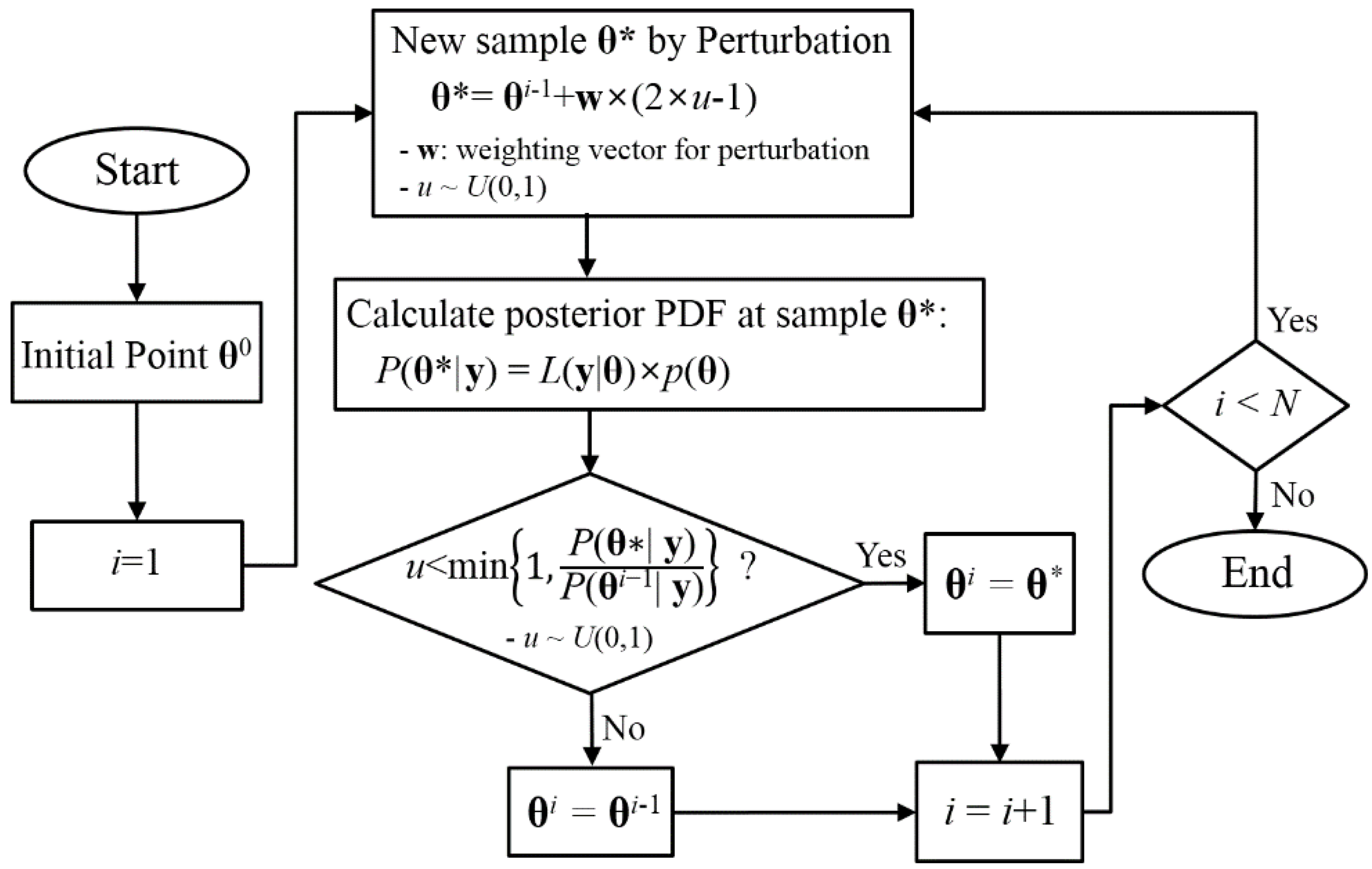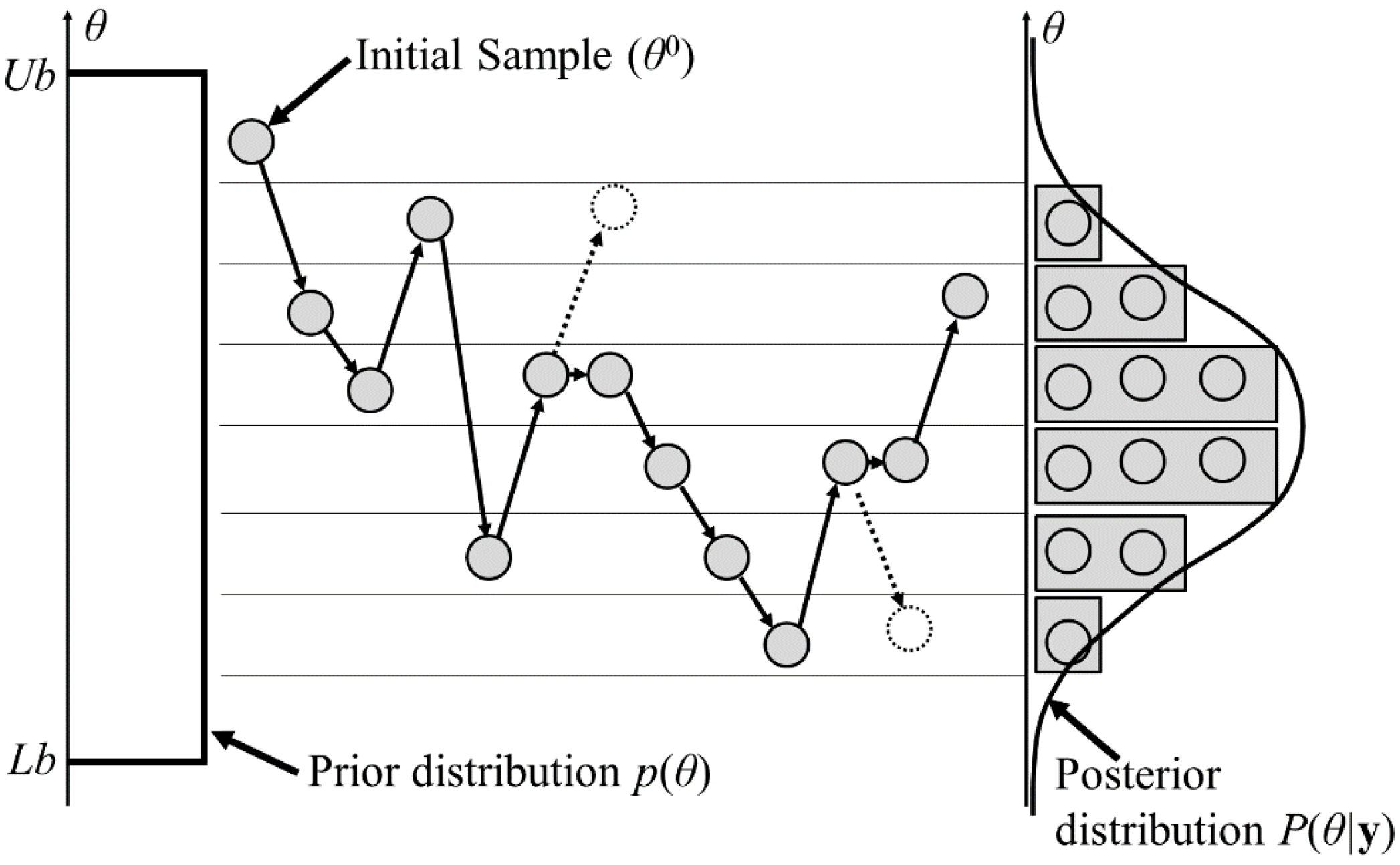[13] carried out a Markov Chain Monte Carlo (MCMC) simulation by generating samples that satisfied the probability distributions and then running a simulation for each sample to capture the probabilistic nature of parameter uncertainties. However, the parameter estimation was not conditional on battery-state data. In Ramadesigan et al. [14], the effective parameters and their uncertainties were estimated in the form of samples based on battery data, using the Bayesian approach and a mathematical reformulation of a porous electrode model. In their study, however, the computation cost to simulate the model with such large samples is not clearly stated; it is likely very high, which may limit its applicability to the on-board vehicle BMS.

Therefore, the purpose of this paper is to propose an efficient method to estimate battery capacity fade, including uncertainty factors. This method could then be easily integrated into the vehicle BMS. The pseudo-two dimensional (P2D) electrochemical model is employed, which simulates the battery state under the profile of the input current by solving a system of coupled nonlinear partial differential equations (PDEs). 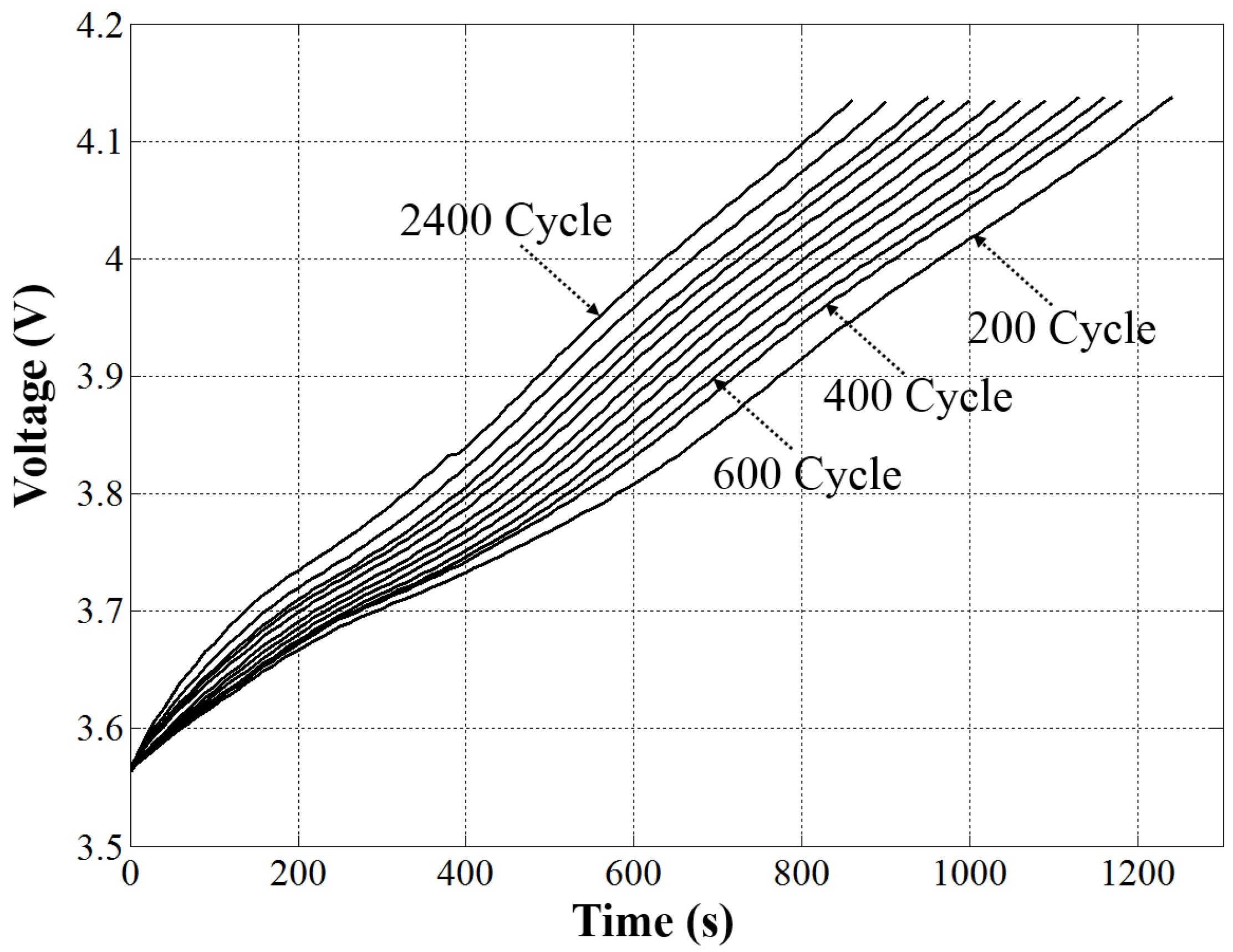The reliability of this electrochemical model has been validated by experiments in which the simulated and measured voltage curves were compared under various charge and discharge conditions [15]. Rather than using data at discharge cycles, which usually undergo arbitrary conditions, this study uses the data at charge cycles, which tend to occur under a constant C-rate. By comparing the simulated and experimental voltage curves, the model parameters representing degradation are estimated by way of large samples to reflect their probabilistic nature.

In order to incorporate the uncertainties in the capacity fade estimation, probabilistic approach is needed, from which the confidence bounds can be determined. In that case, the results are given by the probability distributions instead of a deterministic value. In the practical implementation, a large number of samples (at least 5000) are necessary to represent the distributions, which means that the P2D model should be solved that number of times. Even though a single computation to solve a P2D model only takes a few seconds, it can take several hours to implement the whole number of P2D solutions, which is intractable from a practical viewpoint. Thus, a polynomial-based metamodel is developed to replace P2D electrochemical model. The output variable of the metamodel is the voltage at discrete time steps, and the input variables are the physical parameters such as diffusion coefficients and reaction constants. For the additional alleviation of the computational burden, only one dominant variable is selected as the input variable of the metamodel, and the operating current condition is fixed as the charging cycle with constant C-rate. Note that the computational environment of vehicle BMS is extremely limited. Once the dominant parameter is estimated using the polynomial metamodel, a conservative capacity fade boundary can be determined in the vehicle’s BMS at the 95% confidence level, which represents the safety margin reflecting the uncertainty.

The outline of this paper is as follows: in Section 2, the physical parameters of the LIB electrochemical model are estimated using a Bayesian-based probabilistic approach. The estimation is performed for five transport and kinetic factors that are the principal parameters affecting capacity fade. The estimation results reveal that one parameter dominates in determining capacity fade, which means that this parameter alone can be used to monitor SOH. The metamodel for the selected parameter is constructed in Section 3. The validity of the metamodel is proven through the comparison of voltage curves, and thus the metamodel with its acceptable error can replace the original electrochemical model. Section 4 shows the parameter estimation results obtained using the generated metamodel. The estimated results are again similar to those produced by the original electrochemical model. However, with the metamodel, the computational cost is reduced from 5.5 h to only a few seconds. This huge reduction in computational cost enables us to integrate SOH monitoring into a vehicle BMS, based on physical parameter estimation. Finally, Section 5 summarizes the paper’s conclusions.

2. Parameter Estimation

This section presents the parameter estimation of the LIB electrochemical model. In more detail, the physical parameters of the P2D electrochemical model are estimated using a distribution based on Bayesian inference. The estimation is performed by comparing the voltage curves: (a) measured from the experiments and (b) obtained by solving the model equation. In this section, the LIB electrochemical model [16,17,18] is explained briefly. Then the MCMC method for parameter estimation is introduced. Finally, the estimation results are presented and discussed. From the parameter estimation results, the critical parameter of the LIB electrochemical model is determined.

2.1. Pseudo-Two Dimensional Electrochemical Model

The P2D electrochemical models that simulate the state of the LIB are well described in [16,17,18]. The model aims to obtain the output voltage curve with respect to time when applying the profile of the input current by calculating state variables such as electric potential φ, Li-ion concentration c, and molar flux j of Li at the surface of the spherical particles of active material. These state variables can be calculated by solving a system of coupled nonlinear PDEs [16,17,18], which represent the electrochemical phenomenon occurring in the LIB. The various numerical methodologies to solve a system of equations efficiently have been reported in [15,19,20]. The equations for the electrochemical model include the physical parameters θ, which represent the geometric parameters and transport and kinetic properties. Among the parameters, those that mainly affect capacity fade are selected as targets of the estimation for SOH monitoring. In this work, five transport and kinetic parameters are chosen per the study by [15]: (1) the liquid-phase diffusivity of Li-ion D_e, the solid-phase diffusivities of Li in the (2) positive D_sp and (3) negative D_sn electrodes, and the electrochemical reaction rate constants in the (4) positive k_p and (5) negative k_n electrodes. The effective solid-phase diffusivity was believed to be able to best describe the Li transport through the porous electrode as it is a function of almost all relevant parameters such as Li’s molecular diffusivity, porosity and tortuosity. Similarly, the electrochemical reaction rate constant was considered to be able to represent the charge transfer across the SEI, which is also effective as it is inclusive of the true electrochemical reaction rate constant and the surface area available for electrochemical reactions [12]. The selected five transport and kinetic parameters are estimated by using MCMC method based on the measured voltage data.

2.2. The MCMC Approach for Parameter Estimation

The approach for parameter estimation is based on Bayesian inference, which updates a hypothesis as more observational data are acquired [21,22]. Specifically, the posterior probability density function (PDF) of the model parameter θ = {D_e, D_sp, D_sn, k_p, k_n}, which is conditional on the measured data y, i.e., P(θ|y), can be calculated by Bayes’ rule:

$$P\left(\text{θ}|\text{y}\right)\propto L\left(\text{y}|\text{θ}\right)p(\text{θ})$$

(1)

where L(y|θ) is the likelihood function of the data y conditional on θ, and p(θ) is the prior distribution of θ. The rule states that the degree of likelihood based on unknown parameters is given by the updated or posterior PDF conditional on the data y, which consists of the prior likelihood p(θ) and the likelihood of the data y. In this work, the data y become the vector of measured voltage V_k at discrete time intervals t_k (k = 1,2,…,n). The likelihood function for kth data y_k (i.e., L(y_k|θ)) can be defined based on the assumption that the error of the data against the model follows the normal distribution:

$$L\left(y_k|\mathrm{\theta },\sigma \right)=\frac{1}{\sigma \sqrt{2\pi }}\exp \left\{-\frac{1}{2}\frac{{(y_k-y^k(\mathrm{\theta }))}^2}{{\sigma }^2}\right\}$$

(2)

where σ is the standard deviation and y^k(θ) is the model value corresponding to observed data y_k, which, in this work, is the electrochemical model voltage at interval k. The equation represents the PDF value of the observation y_k with the mean being y^k(θ) and the standard deviation σ based on the assumption of normal distribution. The symbol | represents that the PDF of y_k is given conditional on the parameters y^k(θ) and σ. The joint likelihood function L(y|θ) of the voltage data y becomes the multiplier of the data at whole-number intervals:

$$L\left(\text{y}|\text{θ},\sigma \right)={\displaystyle \prod _{k=1}^{n}L\left(y_k|\text{θ},\sigma \right)}=L\left(y_1|\mathrm{\theta },\sigma \right)\times L\left(y_2|\mathrm{\theta },\sigma \right)\times \mathrm{...}\times L\left(y_n|\mathrm{\theta },\sigma \right)$$

(3)

The prior distribution for θ, and σ in this work is set as the uniform distribution function U between the upper bound Ub and the lower bound Lb:

$$p\left(\mathrm{\theta },\sigma \right)=U(Lb,Ub)$$

(4)

Note that the standard deviation σ is also unknown and estimated from the process. As a result, the unknown parameters consists of the five model parameters θ={D_e, D_sp, D_sn, k_p, k_n} and the standard deviation ion σ is also unknown and estimated from the process.y. The final joint posterior PDF of the unknown parameters is then revised from Equation (1) to:

$$P\left(\text{θ},\sigma |y\right)\propto L\left(y|\theta ,\sigma \right)p(\theta ,\sigma )$$

(5)

From this point on, the unknown parameters will be denoted by a single symbol θ by including σ in it. The posterior PDF P(θ|y) can be effectively evaluated using the MCMC approach, which is widely used as a sampling method in modern computational statistics [21,22]. The MCMC approach is based on the fact that the PDFs built by the Markov Chain process converge on the actual distribution as the sample size increases. Among various sampling method for the MCMC approach, the Metropolis-Hastings (M-H) algorithm is the most representative method applied in this work [23]. The flowchart and illustration of the M-H algorithm are given in Figure 1 and Figure 2, respectively. As shown in Figure 1, the M-H algorithm finds N large samples of the model parameter θ, using a process that includes variate generation and comparison. First, we start with an arbitrary initial sample θ. Then, a new parameter sample θ^* is obtained by calculating a random variate from the parameter sample in the previous step θ^i-1 using the weighting vector w and randomly sampled value u from the uniform distribution between 0 and 1, i.e., U(0,1). Next, the posterior PDF conditional on the measured data y is calculated at the variate θ^*. Then, the ratio of the posterior PDF of the new sample θ^* and the previous sample θ^i-1 (i.e., P(θ^*|y)/P(θ^i-1|y) is compared with the randomly sampled value u from the uniform distribution between 0 and 1, i.e., U(0,1). If the ratio is larger than u, the sample at the current step θⁱ becomes variate θ^*. Otherwise, the sample at the current step θⁱ reverts to the value for the old sample at the previous step θ^i-1. By repeating the process, N samples of the model parameters are calculated, and the posterior PDF P(θ|y) is determined by counting the number of samples at each interval. The conceptual illustration of the M-H algorithm is presented in Figure 2.

Figure 1. Flowchart of Metropolis-Hastings (M-H) algorithm for the parameter estimation using the Markov Chain Monte Carlo (MCMC) approach.

Figure 1. Flowchart of Metropolis-Hastings (M-H) algorithm for the parameter estimation using the Markov Chain Monte Carlo (MCMC) approach.

Figure 2. Illustration of Metropolis-Hastings (M-H) algorithm explained in Figure 1.

Figure 2. Illustration of Metropolis-Hastings (M-H) algorithm explained in Figure 1.

2.3. Parameter Estimation Result

The parameters for the electrochemical model are estimated using the MCMC approach with the M-H algorithm explained previously. The Li-ion cells used in this work are large-formatted with a nominal capacity of 42.5 Ah. Each cell consists of 21 positive electrodes and 22 negative electrodes; those are all two-sided. The active materials of the positive and negative electrodes are composite LiNi_1/3Mn_1/3Co_1/3O₂-LiMn₂O₄ (NMC-LMO) and natural carbon, respectively. The electrolyte consists of LiPF₆ salt in a tertiary solvent mixture of ethylene carbonate (EC), ethyl methyl carbonate (EMC) and diethyl carbonate (DEC). Each of the 21 positive electrodes is bagged by a separator and each of the 22 negative electrodes is sandwiched between the 21 positive electrode-containing separator bags. The entire assembly of positive and negative electrodes and separator is finally enclosed by a pouch. The cycling experiment is performed at 45 °C in 2C-rate condition with full charge and discharge cycles, which leads to capacity degradation. The reason for employing 2C-rate is because the rapid charge is usually made at 2C-rate. Full charging occurs until an end-of-charge voltage of 4.2 V is reached followed by constant voltage charging at 4.2 V until the current tapers down to 0.0235 C-rate. An hour later, the cycle continues with the constant current discharge at a 2C-rate down to a cut-off voltage of 2.5 V.

Note that although the discharge in this work occurs at a constant rate, the battery generally experiences arbitrary loading conditions. On the other hand, charging always takes place at a constant rate. In this sense, use of the data during charge is more desirable for estimation of parameters. The voltage data are collected every 10 s from beginning to end of the constant current charge process. Voltage profiles are taken at 200-cycle intervals between 200 and 2400 cycles. So the 12 data sets are obtained for the voltage profiles as shown in Figure 3. As the cycle progresses, the curve shifts to the left, which indicates that the time required to attain full charge is gradually reduced, resulting in capacity fade. Table 1 presents capacity fade percentage with respect to cycle number. Capacity fade occurs almost linearly as the cycling number increases.

Figure 3. Voltage charge curve at various cycles in the battery experiment at 45 °C in 2C-rate condition with full charge and discharge.

Figure 3. Voltage charge curve at various cycles in the battery experiment at 45 °C in 2C-rate condition with full charge and discharge.

Table 1. Capacity fade (%) with respect to the cycle number.

Cycle number	Fade %	Cycle number	Fade %
200	5.5	1400	19.7
400	9.0	1600	21.3
600	11.4	1800	23.3
800	13.6	2000	24.9
1000	15.8	2200	27.4
1200	17.7	2400	30.3

Table 1. Capacity fade (%) with respect to the cycle number.

Cycle number	Fade %	Cycle number	Fade %
200	5.5	1400	19.7
400	9.0	1600	21.3
600	11.4	1800	23.3
800	13.6	2000	24.9
1000	15.8	2200	27.4
1200	17.7	2400	30.3

Based on the approach in Section 2.2, the unknown parameters at each given cycle are estimated based on the voltage data using the MCMC algorithm. The results are given in Figure 4 for the case at 1200 cycles. In the MCMC process, as was noted in the procedure at lines 22–32, the sampling starts with an arbitrary initial value. Although the MCMC technique is less affected by the initial values due to the unique algorithm of random walk which ensures the sampling convergence toward the target distribution, it is advised to choose the initial values at higher likelihood such as the mean or median of the distribution. In this study, to this end, the initial values of P2D model parameters are given by finding out the solution that minimizes the sum square error (SSE) between the data and the model:

$$\underset{\theta }{\min } {\mathit{SS}}_E={\displaystyle {\sum }_{k=1}^n{(y_k\mathbf{-}{y}^k(\text{θ}))}^2}$$

(6)

Then the initial value of the standard deviation is chosen from the square root of SSE, which is 0.004. The upper bound Ub and the lower bound Lb in Equation (4) are set as 0.4 and 5 times of the initial values of each parameter, respectively. The total number of samples in M-H algorithm is set as 10,000. The upper histograms in Figure 4 represent the PDF thus obtained. The lower plots represent plot the samples until the end of the MCMC iteration. Note that the first 1000 samples that are affected by the initial distribution are considered a burn-in period and are discarded [21]. The results as shown in this figure give more valuable information for the estimated parameters because they incorporate the uncertainties in both model and measurements, which is contrasted with the deterministic optimization that gives only point-estimated values.

Figure 4. Parameter estimation as a result of voltage data at cycle 1200 (capacity fade 17.7%). The upper histograms show the number of samples of the M-H algorithm over the probable range, which represents the estimated PDF. The lower plots show the values of each parameter up to 10,000 iterations, as explained in Figure 2: (a) liquid-phase diffusivity D_e; (b) solid-phase diffusivity in the positive electrode D_sp (c) solid-phase diffusivity in the negative electrode D_sn; (d) electrochemical reaction-rate constant in the positive electrode k_p; (e) reaction-rate constant in the negative electrode k_n; (f) standard deviation σ of the likelihood function.

Figure 4. Parameter estimation as a result of voltage data at cycle 1200 (capacity fade 17.7%). The upper histograms show the number of samples of the M-H algorithm over the probable range, which represents the estimated PDF. The lower plots show the values of each parameter up to 10,000 iterations, as explained in Figure 2: (a) liquid-phase diffusivity D_e; (b) solid-phase diffusivity in the positive electrode D_sp (c) solid-phase diffusivity in the negative electrode D_sn; (d) electrochemical reaction-rate constant in the positive electrode k_p; (e) reaction-rate constant in the negative electrode k_n; (f) standard deviation σ of the likelihood function.

In comparing the estimated PDFs of each parameter, the PDF of D_sp is noted to be much narrower than that of the other parameters. This narrower PDF means that the uncertainty of the parameter D_sp is much lower than that of the other parameters for the given data set. The estimation using the MCMC approach is performed for all 12 data sets obtained from between 200 and 2400 cycles in 200-cycle increments. From the obtained histogram representing the PDF, the 95% confidence interval and mean value are calculated and plotted in Figure 5 as a function of the capacity fade %. The figure shows that the parameter D_sp decreases considerably with narrower confidence bounds than the others as capacity fade progresses. Thus there is a strong correlation between D_sp and capacity fade, indicating that D_sp is the dominant parameter affecting capacity fade for the given data set.

Figure 5. Interval estimation results of battery parameters as capacity fade progresses from 5.5% (cycle 200) to 30.3% (cycle 2400). The 95% confidence intervals and mean values are presented for each model parameter: (a) D_e; (b) D_sp; (c) D_sn; (d) k_p; (e) k_n; (f) σ.

Figure 5. Interval estimation results of battery parameters as capacity fade progresses from 5.5% (cycle 200) to 30.3% (cycle 2400). The 95% confidence intervals and mean values are presented for each model parameter: (a) D_e; (b) D_sp; (c) D_sn; (d) k_p; (e) k_n; (f) σ.

3. Metamodel Generation

The metamodel approximates the original complex model with simplified, explicit functions. In this study, the metamodel can replace the complex electrochemical model to reduce computational cost during parameter estimation by using the MCMC approach. In this section, the Response Surface Method (RSM) used to generate the metamodel is explained. Then the generated model is validated by comparing the voltage curves of both metamodel and the original electrochemical model.

3.1. Response Surface Method

The RSM is a representative way to generate the metamodel [24]. The steps for generating the metamodel are as follows. First, output function values at multiple input sample points are evaluated from the original complex models. Considering the trend of output function values with respect to the input variables, the form of the approximated mathematical function is determined. Finally, the coefficients of the approximated function are found, based on the least-squares method.

In this study, the solid-phase diffusivity in positive electrode D_sp is the only input variable of the metamodel. The terminal voltage is set as the output function because it is the single most critical parameter for the change of the voltage curve as capacity fade occurs. Four other model parameters are fixed at their mean values, which are obtained using cycle-200 experimental data. By employing only one parameter D_sp instead of all five, the complexity of the metamodel can be greatly reduced. In order to validate the complexity reduction, P2D simulations are carried out every 200 cycles, first using all five estimated parameters and then using only one estimated parameter D_sp with the other four fixed at their mean at cycle 200. Because the parameters and responses are all given by distributions, only the means of the voltage outputs are plotted against the experimental data for the sake of easy comparison. Figure 6 shows the results (a) using all the five model parameters and (b) using only D_sp.

Figure 6. Comparision of the voltage obtained from the P2D model with experimental data. The dots represent the simulated result using the mean of estimated parameters: (a) all five model parameters estimated from experimental data; (b) only D_sp estimated while other parameters are fixed at mean value of cycle 200.

Figure 6. Comparision of the voltage obtained from the P2D model with experimental data. The dots represent the simulated result using the mean of estimated parameters: (a) all five model parameters estimated from experimental data; (b) only D_sp estimated while other parameters are fixed at mean value of cycle 200.

At each cycle i, the relative error e_i of the output voltage against the experimental data is defined as:

$$e_i=\frac{1}{n} [{\displaystyle \mathbf{\sum }_{k=1}^n \left|\frac{{V_{ki}}^{*}-V_{ki}}{V_{ki}}\right|} ] \times 100 (\%)$$

(7)

where V_ki^* and V_ki are model output and experimental data at the time interval t_k (k = 1~n) and ith cycle number, respectively. The error e_i is calculated at cycles 200, 800, 1600, and 2400 for each case, and the results are summarized in the first and second row in Table 2.

Table 2. Error e_i of the model with respect to experimental data.

	Cycle 200	Cycle 800	Cycle 1600	Cycle 2400
P2D w/5 parameters (Figure 6a)	0.195%	0.142%	0.110%	0.078%
P2D w/ Dsp (Figure 6b)	0.195%	0.332%	0.346%	0.262%
Metamodel (Figure 7)	0.210%	0.310%	0.351%	0.241%

Table 2. Error e_i of the model with respect to experimental data.

	Cycle 200	Cycle 800	Cycle 1600	Cycle 2400
P2D w/5 parameters (Figure 6a)	0.195%	0.142%	0.110%	0.078%
P2D w/ Dsp (Figure 6b)	0.195%	0.332%	0.346%	0.262%
Metamodel (Figure 7)	0.210%	0.310%	0.351%	0.241%

The greatest error value, a maximum of 0.346%, is produced by only one parameter, as compared with the maximum value of 0.195% by the five parameters. However, the difference in magnitude is small enough to justify that the parameter D_sp can be used as the single input variable of the metamodel. The metamodel of the P2D electrochemical model is built using RSM. First, the response data are obtained using the original P2D electrochemical model, which is the terminal voltage V_ki at discrete time intervals t_k (k = 1~n) and at m equally spaced discrete input variables D_sp;i (I = 1~m). In this study, the interval of the metamodel is 50 s, n = 24, and the end time is 1200 s. The number m is set as 10, with the lower and upper bounds D_sp;1 and D_sp;10 being 0.5 10⁻¹⁵ and 2.5 × 10⁻¹⁵ respectively, considering the behavior of D_sp in Figure 5b. In Figure 8, the obtained response values V_ki are plotted as dots at the discrete values of the variable D_sp and time t. From the figure, it can be seen that the voltages at fixed intervals t_k decrease monotonically with respect to D_sp. So, a simple polynomial is introduced to represent voltage as a function of D_sp at each discrete interval.

Figure 7. Comparision of the voltage obtained from the metamodel with experimental data.

Figure 7. Comparision of the voltage obtained from the metamodel with experimental data.

Figure 8. Output voltage with respect to input variable D_sp for various time intervals. The red dot represents the voltage V_ki at D_sp and interval t_k;i as obtained from the P2D model; the solid black line represents the voltage curve V_k(D_sp) obtained using fourth-order polynomials in the metamodel.

Figure 8. Output voltage with respect to input variable D_sp for various time intervals. The red dot represents the voltage V_ki at D_sp and interval t_k;i as obtained from the P2D model; the solid black line represents the voltage curve V_k(D_sp) obtained using fourth-order polynomials in the metamodel.

After calculating the error between metamodel and original model, the order of the polynomials is determined to be fourth degree. Then the voltage curves at time t_k are represented as:

$$V_k(D_{sp})={\displaystyle \mathbf{\sum }_{p=1}^4{a}_{kp}{D_{sp}}^p}=a_{k0}+a_{k1}{D}_{sp}+a_{k2}{D_{sp}}^2+a_{k3}{D_{sp}}^3+a_{k4}{D_{sp}}^4$$

(8)

In the above equation, the coefficients a_kp at time t_k, with p being the polynomial order, are calculated to match with the original response data, using the least-squares method. Because the polynomial function is linear with respect to the coefficients a_kp, a typical linear regression algorithm can be used, in which the m-by-5 matrix X is defined as:

$$\mathrm{X}=\frac{\partial V_k(D_{e;i})}{\partial a_j}=\left[\begin{array}{cccc}1& D_{e;1}& \cdots & {D_{e;1}}^4\\ 1& D_{e;2}& & {D_{e;1}}^4\\ ⋮& ⋮& & ⋮\\ 1& D_{e;m}& \cdots & {D_{e;m}}^4\end{array}\right]$$

(9)

Then, the 5-by-m matrix a can be obtained as:

$$\text{a}=a_{kp}=\left[\begin{array}{cccc}{a}_{10}& a_{20}& \cdots & a_{n0}\\ a_{11}& a_{21}& & a_{n0}\\ ⋮& & & ⋮\\ a_{14}& a_{24}& \cdots & a_{n0}\end{array}\right]={({\mathrm{X}}^T\mathrm{X})}^{-1}{\mathrm{X}}^T\text{y}$$

(10)

where y denotes the m-by-n matrix composed of V_ki corresponding to ith input variable D_sp;i at kth time interval t_k:

$$\mathrm{y}=V_{ki}=\left[\begin{array}{cccc}{V}_{11}& V_{21}& \cdots & V_{n1}\\ V_{12}& V_{22}& & V_{n2}\\ ⋮& & & ⋮\\ V_{1m}& V_{2m}& \cdots & V_{nm}\end{array}\right]$$

(11)

In Figure 8, the solid black line represents the metamodel in which the voltage curve V_k is given by the fourth-order polynomial with respect to the input variable D_sp. This model is used instead of the original electrochemical model to gain computational efficiency during the MCMC sampling process.

3.2. Model Validation

The generated metamodel is validated by comparing the metamodel’s output voltage with the corresponding experimental data for various cycles. The result of the comparison is presented in Figure 7, which shows that the metamodel describes the voltage curve of the experimental data well. To evaluate the accuracy of the metamodel against the original P2D model, the error e_i as defined by Equation (7) is calculated for the metamodel at the cycles 200, 800, 1600 and 2400, and the results are given in the third row of Table 2. The errors of the metamodel and the P2D model with one parameter show similar magnitude, with the maximum being about 0.35%.

4. Parameter Estimation Using the Metamodel

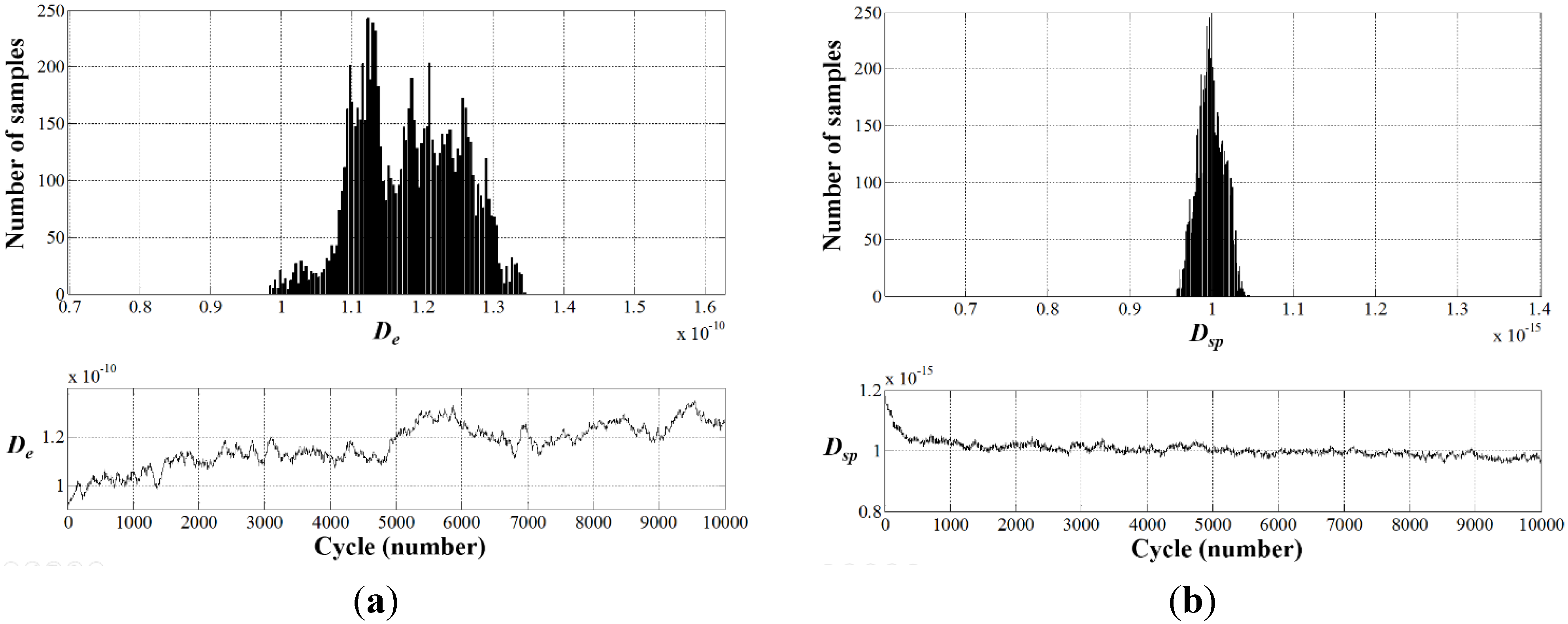
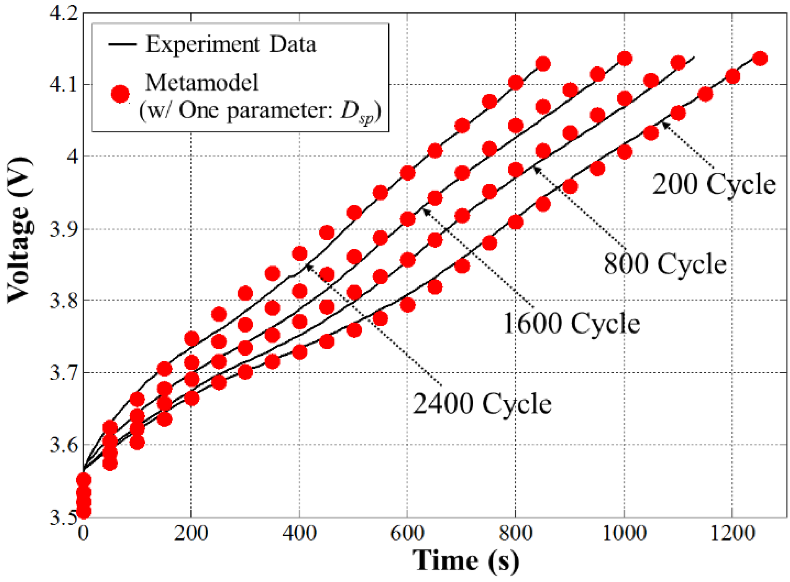
Based on the generated metamodel, the parameter estimation is again performed using the MCMC approach, and the estimation result is presented in Figure 9, in which the 95% confidence interval and mean value are plotted as a function of the capacity fade %. Please note that only one estimated parameter D_sp in Figure 9 includes all the sources of uncertainty. The various uncertainties are involved in one estimated parameter through the standard deviation σ. Here, the standard deviation σ is set as 0.05 V considering the uncertainty of the experimental data. Next, the estimated parameters are applied to the metamodel’s voltage curve to obtain capacity fade in the form of distribution, from which the upper and lower bounds are calculated. The results in Figure 10 are given in terms of cycles at a 200-cycle increment. Using the metamodel based on fourth-order polynomials instead of the original P2D model that solves a system of nonlinear PDEs, the computational cost is tremendously reduced.

Figure 9. Parameter (D_sp) estimate using metamodel (see Figure 5b).

Figure 9. Parameter (D_sp) estimate using metamodel (see Figure 5b).

Figure 10. Capacity-fade estimation using the metamodel over the cycles.

Figure 10. Capacity-fade estimation using the metamodel over the cycles.

Given 10,000 samples, the original model’s computing time is 5.5 h (about 2 s per sample) on an octacore workstation with a 3.4 GHz processor and 16 GB of RAM. However, the same computation takes only a few seconds using the metamodel. Thanks to this reduction, the integration of the proposed approach into a vehicle BMS becomes a feasible option.

5. Conclusions and Future Work

This study proposes an efficient method of uncertainty estimation of capacity fade in LIBs, with the goal of integrating it into the BMS of electric vehicles. The physical parameters of the LIB electrochemical model are estimated using the Bayesian-based probabilistic approach. The estimation is performed for five transport and kinetic parameters that are known to affect capacity fade most significantly. Battery data from the full charge/discharge cycles with 2C-rate condition are utilized to implement the method. From the estimation, it is found that one parameter, the solid-phase diffusivity in the positive electrode, is much more responsible than the others for capacity fade. The metamodel is constructed in terms of this parameter in order to avoid the huge computations that occur in the P2D model for MCMC simulation. As a result, computation cost is reduced from 5.5 h to only a few seconds. The reduction of computation time allows the uncertainty estimation of the parameters in real time during battery use, which adds value to the BMS relative to safety and reliability.

This study considers only the case of 2C-rate full charge/discharge process to illustrate the method, in which the data at charge cycle are used for the capacity-fade estimation. The reason for 2C-rate is to accelerate the cycles. In practice, the rapid charge is usually made at 2C-rate. Therefore, the constructed metamodel works only under the same charge condition. In other words, as long as the parameters are estimated under the same charge condition during usage, the estimated results are reliable and represent the actual faded state at that cycle, regardless of the discharge condition the battery went through. If another C-rate (e.g., the normal 1C-rate) is used for charging, the metamodel can be constructed using the same procedure and applied to that condition. As a result, two models with different C-rate conditions can be installed in one BMS and can be used as appropriate to estimate capacity fade.

In this study, only the full-charge condition is addressed. In actual practice, however, the range of completely charged to completely discharged is never available, and a partial charge is more realistic. The proposed method is unable to estimate in this case, which is a challenge to be addressed in future work.

References

1. Americans want to give electric vehicles a test drive. New CEA study reports. CARS Magazine, 23 August 2010.
2. Xing, Y.; Ma, E.; Tsui, K.L.; Pecht, M. Battery management system in electric and hybrid vehicles. Energies 2011, 4, 1840–1857. [Google Scholar] [CrossRef]
3. He, W.; Williard, N.; Osterman, M.; Pecht, M. Prognostics of lithium-ion batteries based on Dempster-Shafer theory and the Bayesian Monte Carlo method. J. Power Sources 2011, 196, 10314–10321. [Google Scholar] [CrossRef]
4. Williard, N.; He, W.; Osterman, M.; Pecht, M. Comparative analysis of features for determining state of health in lithium-ion batteries. Int. J. Progn. Health Manag. 2013, 4, 1–7. [Google Scholar]
5. Barre, A.; Deguilhem, B.; Grolleau, S.; Gérard, M.; Suard, F.; Riu, D. A review on lithium-ion battery ageing mechanisms and estimations for automotive applications. J. Power Sources 2013, 241, 680–689. [Google Scholar] [CrossRef]
6. Rezvanizaniani, S.M.; Liu, Z.; Chen, Y.; Lee, J. Review and recent advances in battery health monitoring and prognostics technologies for electric vehicle (EV) safety and mobility. J. Power Sources 2014, 256, 110–124. [Google Scholar] [CrossRef]
7. Chaturvedi, N.A.; Klein, R.; Christensen, J.; Ahmed, J.; Kojic, A. Algorithms for advanced battery-management systems. IEEE Control Syst. 2010, 30, 49–68. [Google Scholar] [CrossRef]
8. Marcicki, J.; Canova, M.; Conlisk, A.T.; Rizzoni, G. Design and parametrization analysis of a reduced-order electrochemical model of graphite/LiFePO 4 cells for SOC/SOH estimation. J. Power Sources 2013, 237, 310–324. [Google Scholar] [CrossRef]
9. Baek, K.W.; Hong, E.S.; Cha, S.W. Capacity fade modeling of a Lithium-ion battery for electric vehicles. Int. J. Automot Technol. 2015, 16, 309–315. [Google Scholar] [CrossRef]
10. Hu, C.; Jain, G.; Zhang, P.; Schmidt, C.; Gomadam, P.; Gorka, T. Data-driven method based on particle swarm optimization and k-nearest neighbor regression for estimating capacity of lithium-ion battery. Appl. Energ. 2014, 129, 49–55. [Google Scholar] [CrossRef]
11. Xiong, R.; Sun, F.; Chen, Z.; He, H. A data-driven multi-scale extended Kalman filtering based parameter and state estimation approach of lithium-ion polymer battery in electric vehicles. Appl. Energ. 2014, 113, 463–476. [Google Scholar] [CrossRef]
12. Hu, C.; Jain, G.; Tamirisa, P.; Gorka, T. Method for estimating capacity and predicting remaining useful life of lithium-ion battery. Appl. Energ. 2014, 126, 182–189. [Google Scholar] [CrossRef]
13. Tong, W.; Koh, W.Q.; Birgersson, E.; Mujumdar, A.S.; Yap, C. Correlating uncertainties of a lithium-ion battery––A Monte Carlo simulation. Int. J. Energ. Res. 2015, 39, 778–788. [Google Scholar] [CrossRef]
14. Ramadesigan, V.; Chen, K.; Burns, N.A.; Boovaragavan, V.; Braatz, R.D.; Subramanian, V.R. Parameter estimation and capacity fade analysis of lithium-ion batteries using reformulated models. J. Electrochem. Soc. 2011, 158, A1048–A1054. [Google Scholar] [CrossRef]
15. Sung, W.; Shin, C.B. Electrochemical model of a lithium-ion battery implemented into an automotive battery management system. Comput. Chem. Eng. 2015, 76, 87–97. [Google Scholar] [CrossRef]
16. Botte, G.G.; Subramanian, V.R.; White, R.E. Mathematical modeling of secondary lithium batteries. Electrochim. Acta 2000, 45, 2595–2609. [Google Scholar] [CrossRef]
17. Gomadam, P.M.; Weidner, J.W.; Dougal, R.A.; White, R.E. Mathematical modeling of lithium-ion and nickel battery systems. J. Power Sources 2002, 110, 267–284. [Google Scholar] [CrossRef]
18. Santhanagopalan, S.; Guo, Q.; Ramadass, P.; White, R.E. Review of models for prediction the cycling performance of lithium ion batteries. J. Power Sources 2006, 156, 620–628. [Google Scholar] [CrossRef]
19. Subramanian, V.R.; Boovaragavan, V.; Ramadesigan, V.; Arabandi, M. Mathematical model reformulation for lithium-ion battery simulations: Galvanostatic boundary condtions. J. Electrochem. Soc. 2009, 16, A260–A271. [Google Scholar] [CrossRef]
20. Ramadesigan, V.; Boovaragavan, V.; Pirkel, J.C.; Subramanian, V.R. Efficient reformulation of solid-phase diffusion in physics-based lithium-ion battery models. J. Electrochem. Soc. 2010, 157, 854–860. [Google Scholar] [CrossRef]
21. Gelman, A.; Carlin, J.B.; Stern, H.S.; Rubin, D.B. Bayesian Data Analysis; Taylor & Francis: London, UK, 2014. [Google Scholar]
22. Andrieu, C.; Freitas, N.D.; Doucet, A.; Jordan, M.I. An introduction to MCMC for machine learning. Mach. Learn. 2003, 50, 5–43. [Google Scholar] [CrossRef]
23. Dawn, A.; Choi, J.H. Improved MCMC method for parameter estimation based on marginal probability density function. J. Mech. Sci. Technol. 2013, 27, 1771–1779. [Google Scholar]
24. Arora, J. Introduction to Optimum Design; Academic Press: Salt Lake City, UT, USA, 2004. [Google Scholar]