1. Introduction
There is a growing awareness that global climate change caused by the increase in greenhouse gas emissions into the biosphere is one of the main challenges in the 21st century. In order to meet the challenge of global climate change and to achieve energy-environment-economy development, the building of a low carbon society is a priority in the national development strategies of many countries. The concept of a low carbon society concerns all aspects of the society, including economy, culture and life [
1]. The European Union (EU) has officially declared that it would cut emissions by at least 80% by 2050 [
2]. Meanwhile, the U.S. and Japan have also made it clear that substantial investment in clean energy development is expected to prompt the reduction of CO
2 emissions by 80% in 2050 compared with those in 2005 [
3]. Developing countries represented by the BRICS nations (Brazil, Russia, India, China and South Africa) have also expressed a strong willingness to control emissions, while putting forward their own specific plans or programs for emission mitigation. According to China’s decarbonisation roadmap, the emissions per unit of gross domestic product (GDP) are required to be reduced by 40% to 45% compared with those in 2005, and renewable energy consumption should account for 15% of the total by 2020 [
4]. However, China’s emissions are more likely to continue rising rapidly in line with its ongoing industrialization and urbanization, which will result in more energy consumption [
5], hence, China will face tremendous challenges in achieving its mitigation targets provided effective measures are not taken. In response, the Chinese central government has made unremitting efforts towards exploring mitigation policies and other measures.
In the context of pursuing climate policy targets for 2020, a number of studies are underway to deeply probe different emission abatement policies and assess the corresponding compliance costs. Economists exceptionally value market-based climate management tools, to strive to minimize the economic costs in realizing the given emission reduction goals, and to provide dynamic incentives for long-term development of cheaper abatement technologies. The legislative package is designed to curb carbon emissions and to maintain low-cost abatement incentives in which carbon renewable, taxes and emission trading may all play a prominent role.
There is evidence that a broader set of energy and climate policies must be implemented to lower the abatement costs as much as possible. Research on imposing duties on carbon emissions has been done in the past few decades, mainly to identify the right tax rate that would help reduce carbon emissions with the lowest adverse impact on economic operations, and consequently alleviate climate change [
6,
7,
8]. Emission trading is the most important regulatory instrument that makes emission allowances obligatory for CO
2 emissions from electricity generation as well as energy-intensive industries [
9,
10,
11]. There is extensive literature on emission reduction targets, possible mitigation policies and costs in developed countries [
12,
13], but few studies are focused on the impacts of energy and climate policies in the context of emission mitigation in China. Undoubtedly, it is very necessary to quantitatively assess the potential results of the deployment of mitigation policies to reach the objective of impacting both the national economy and the energy mix to a large extent. Impact assessments of emission reduction commitments and non-fossil energy target plans for 2020, have been performed in [
5,
14].
Currently, renewable energy, considered as the main way to achieve energy savings and emission cuts, will see a substantial expansion over the next several decades. Subsequently, under a reasonable policy guidance for key economic sectors, technological changes will have great economic implications through improving energy efficiency whilst reducing the reliance on fossil fuels and cutting emission intensity [
15]. Different from the carbon market in developed countries, an absolute cap on emissions needs to be set in China, which is eventually to be implemented by the different sectors and enterprises. Both carbon taxes and ET encourage enterprises to mitigate emissions in the production process by means of market forces. It is expected that timely introduction of a carbon tax from 2015 to 2020 which will achieve its impact through price measures will curb mounting emissions, while emission trading, a cap mechanism based on market competition, provides cost-effective and flexible environmental compliance for energy systems.
Increases of carbon emissions and their possible negative effects are major concerns in the imposition of any policy strategy [
16]. Considering that climate policies including renewable energy plans, carbon taxes and emission trading are particularly helpful to combat climate change, it is very necessary to investigate the implications of alternative climate policies on economic and social development, so as to consequently provide policy recommendations for the state.
In recent years, as a popular policy simulation tool, computable general equilibrium (CGE) models have been widely employed in the analysis of climate policy, in particular, the assessment of long-term effects on economic consequences, sector productivity and energy systems [
14,
17,
18]. This study aimed to provide an in-depth analysis of these mitigation measures, especially the impacts of renewable energy, ET and carbon taxes, on economic development, sectoral output, energy systems,
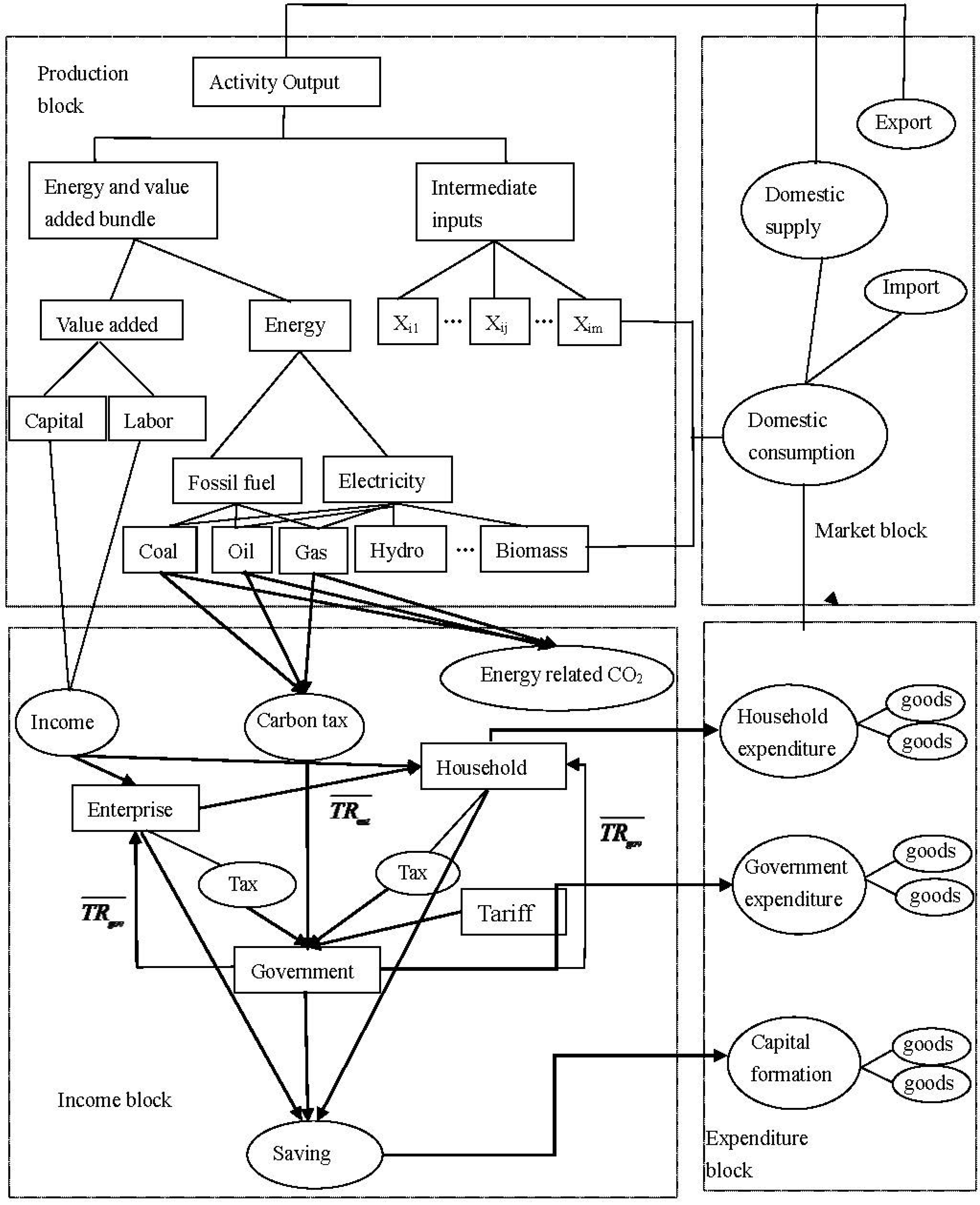
etc. by establishing a new and revised hybrid static Asia-Pacific Integrated Model/computable general equilibrium (AIM/CGE) model.
The analysis is organized as follows:
Section 2 briefly describes the AIM/CGE model and design scenarios.
Section 3 presents the acquired simulation results, including the impacts of mitigation commitment on GDP, sectoral output, energy supply, and energy consumption by sectors and by types, energy intensity, carbon intensity and carbon prices and the impacts of different time levels to cancel the electricity price subsidies, increasing carbon taxes and limited emission trading. Finally, the results are summarized in brief, which also shows the useful policy implications of the study.
3. Simulation Results
Our model allows us to assess the impacts of emission mitigation measures on macroeconomics, sector output, energy system and carbon prices. The results of each scenario are presented under the background of three alternative mitigation policies to support the exploration of China’s future mitigation strategy.
3.1. Carbon Intensity
3.1.1. Carbon Intensity in This Model
China’s sky-rocketing energy consumption causes high emissions. The current situation shows that emission mitigation is relatively difficult. Nevertheless, China’s government has made an ambiguous commitment to lower emissions per unit of GDP from 40% to 45% compared with those in 2005. Over the past five years, the total CO2 emissions have increased from 5170 million tons in 2005 to 8332 million tons in 2010, a 61.16% rise. In terms of emissions for GDP per unit from 2005 to 2010, they only dropped from 1.36 to 1.29 tons per 1000 US dollars (t/1000 USD, a 5.14% drop) meaning that there are enormous pressures in achieving reduction targets.
Results of CO
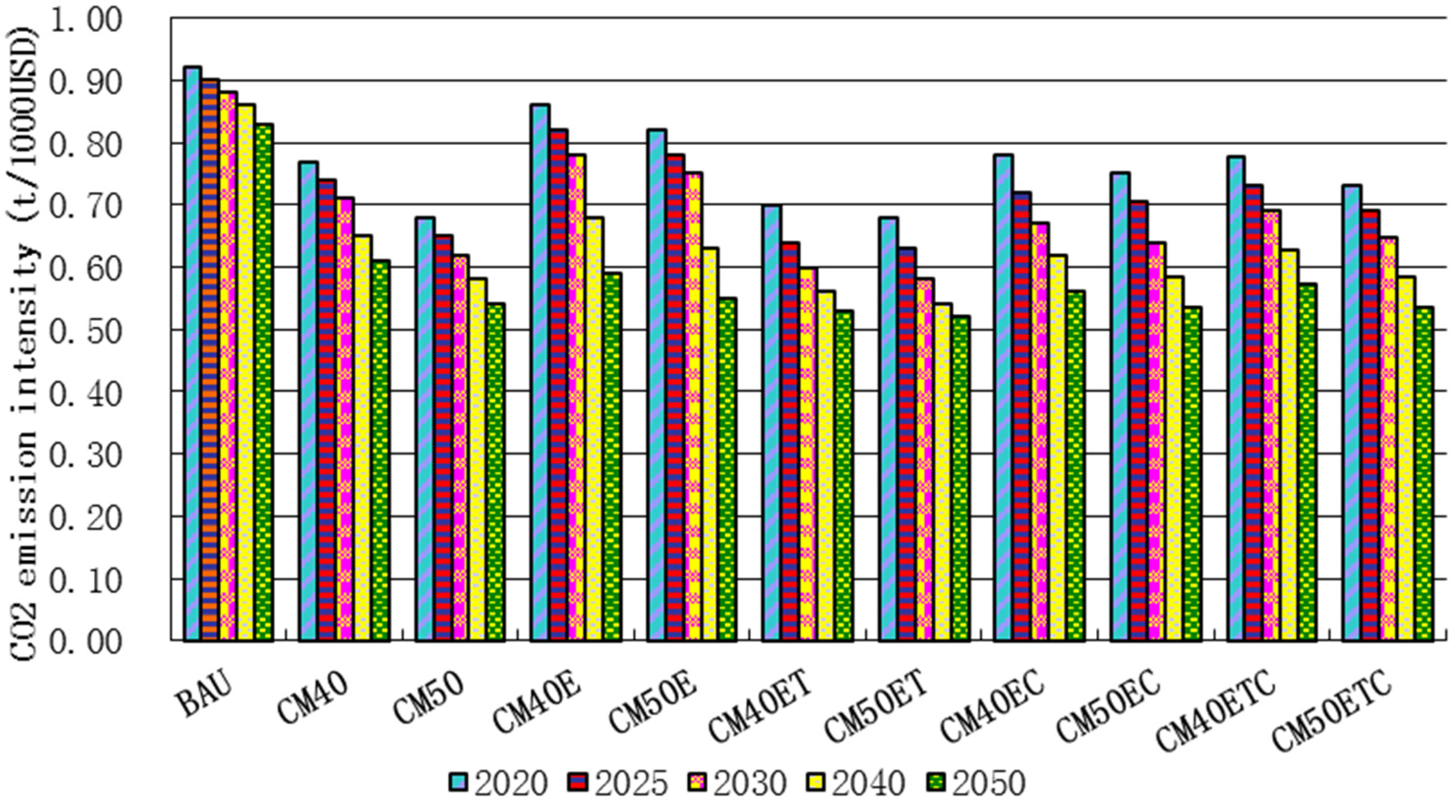
2 emission intensity during 2020–2050 are illustrated in
Figure 3. It is shown that CO
2 emission intensity changes significantly after the deployment of renewable energy, a drop of 33.33% in CM40E and 36.43% in CM50E by 2020, respectively, compared with 1.36 t/1000 USD in 2005. On the basis of renewable energy, emission trading will reduce emission intensity by 43.31% in CM40ET and 46.53% in CM50ET by 2020, which obviously shows a high probability of achieving China’s CO
2 emission mitigation target commitments made in Copenhagen.
The CO2 emissions in the BAU scenario remain on a downward trend, but the value in 2050 is apparently higher than that in other scenarios. The carbon intensity is less than 0.70 t/1000 USD in the scenarios with renewable energy and emission trading, which means that the targets proposed in Copenhagen are achievable. It is apparent that the carbon tax overwhelmingly contributes to lower carbon emissions when implemented. However, the effect of emission trading measures on emission intensity reduction obviously surpasses that of the carbon tax. Besides, the impacts of carbon tax on reducing emission intensity work in the short term, for example, the annual average rate of decrease of emission intensity is 1.1%–1.4% in CM40EC, CM40ETC, CM50EC, and CM50ETC during 2020–2030, while it is only 0.2%–0.5% during 2030–2050. In the short run, energy intensive enterprises have to reduce their production to fulfill the emission reductions in the face of the absolute increase in production costs because fixed costs remain constant and the introduction of new technology or switching to other production may be unrealistic. Therefore, the emission reduction and carbon intensity drop are obvious. However, in the long run, introduced low carbon technology and turning over to other sector makes the carbon tax less efficient. Moreover, energy efficient enterprises lack any motivation to reduce emissions because they pay lower carbon taxes. Hence, the carbon intensity would not sink rapidly in the long term.
Figure 3.
CO2 emission intensity from 2020 to 2050.
Figure 3.
CO2 emission intensity from 2020 to 2050.
In contrast, the emission intensity in scenarios without a carbon tax falls steadily during the research period. The estimated value of emission intensity falls to 0.54 t/1000 USD in CM40ET and 0.52 t/1000 USD in CM50ET, respectively, by 2050. The CM50ECT scenario sees roughly the same effect as CM50ET.
3.1.2. Renewable Energy Subsidies and Carbon Intensity
In the early stages, the development of renewable energy is faced with immense difficulties due to the high costs. Given that renewable energy plays a key role in the development of any national energy strategy, most advanced countries and regions have established appropriate capital subsidy mechanisms. As the largest developing country, China has adopted effective measures to support the development of renewable energy, mainly including renewable energy feed-in tariffs. The continuing financial support for promoting the development of renewable energy will unquestionably increase the government’s financial burden. The tariff subsidies are estimated to be 16.7 billion dollars in 2015 and 25.3 billion dollars in 2020. Tariff subsidies are predictably eliminated based on the renewable energy development trend. Nevertheless, a sober assessment is needed to establish the best specific time to cancel subsidies.
In this study, diverse temporal patterns are used to assess the impacts when the government removes its tariff subsidies at different times. It is assumed that subsidies are removed in 2015, 2020 and 2025, respectively. It shows a marked comparison of carbon intensity in 2050 after removing the tariff subsidies at different times. Results reveal that the early cancellation of subsidies in 2015 curbs carbon intensity reduction in the future, while the abolition of subsidies in 2025 makes little difference. The following reasons may provide a general understanding of this phenomenon. Although the cost of renewable energy is higher than that of fossil energy, renewable energy is the major means to reduce the emissions before 2015. Over the ten years, the development cost of renewable energy has dropped by more than 50%, in particular, the cost of photovoltaic power generation has decreased by 15% every year. The renewable electricity will be cheaper after 2015, which could be acceptable for some enterprises. However, the thermal power generation cost in China is likely to rise because of the increasing coal price. Moreover, in order to achieve the mitigation goals, enterprises are bound to use renewable energy even if it is more expensive because it is still cheaper than the introduction of new technology.
By comparing the scenario of removing subsidies in 2020 with that in 2025, it is found that the margin of carbon intensity reduction in all reduction measures is less than 0.2 t/1000 USD. In other words, the result coincides with experts’ predictions that after 2020, the removal of subsidies is relatively appropriate at least from the perspective of reducing carbon emissions.
3.1.3. Limited Emission Trading and Carbon Intensity
Free emission trading implies that no trade credit and scope will be captive. However, emission trading may be restricted to a certain level. China’s enterprises will be in trouble in free emission trading with other countries, such as the EU, stemming from the gap of production technology. China’s enterprises are always at a disadvantage in market competition due to their technical level. In order to protect domestic firms, limited emission trading may play an important role in accelerating the development of native industries. Therefore, it is significant to explore the impacts of trade constraints on activity level and mitigation.
After a comprehensive analysis and calculation, results convincingly indicate the inappropriate expectations. For protectionist reasons, 50% of the trade is merely restricted to domestic sources but this is unable to produce the desired effect, and worse still, it prevents sectors from raising the level of output. Protectionism prevents enthusiasm for innovation, but is conducive to production technology development. The decline in GDP reaches 1.3% compared with that in the free trade level, unwilling to address this aspect, which means sector activity will be undoubtedly affected, partly due to the technical gap. Surprisingly, carbon emission intensity is not affected much by the carbon taxes deployed in the CM40ETC and CM50ETC scenarios, compared with the average increase of 0.15 t/1000 USD in other scenarios. Obviously, the emission trading for limiting the amount of the transaction does not lower the carbon emission intensity as expected, and instead it causes some adverse effects on economic development and technological progress.
3.1.4. Increasing Carbon Tax and Carbon Intensity
In this study, the carbon tax rate is held at 5 $/t for simplicity sake, however, it is changeable in the practical economic and social context based on the government policies. Therefore, in this section, the carbon tax rate is assumed to increase from 2 $/t to 10 $/t within a decade, after which it remains unchanged and consistent with the current policy direction. The output in the industrial sector accounts for a large proportion of the GDP. As expected, a carbon tax inevitably has an adverse impact on the activity level in the industrial sector. However, the effects of carbon tax can be significantly reduced if a lower tax rate is followed initially in accordance with the deployment of government norms. In addition, the increase of marginal abatement costs is less pronounced. A lower carbon tax serves as a guide in improving the production technology and energy efficiency to some extent. With the increase of tax rate, enterprises will shoulder the pressure of reducing the energy consumption per unit of output to meet the cost increases due to energy consumption.
Simulation results indicate CO2 emission intensity changes with the carbon tax rate gradually increasing from 2 $/t to 10 $/t according to the hypothesis. Compared with fixed rates, incrementing the tax rate contributes to a more substantial reduction in carbon emissions and the consequential drop in carbon intensity. From a practical point of view, higher carbon tax indeed can greatly reduce carbon emissions instead of carbon intensity. Based on the simulation results, emission intensity will see a big decline in CM50EC and CM50ETC, reducing to 0.51 t/1000 USD in CM50ETC, a drop of 0.2 t/1000 USD, however, a higher carbon tax rate has a huge impact on China’s GDP. At the carbon tax rate of 10 $/t, the GDP loss in CM40EC and CM50EC reaches 3.47% and 5.06%, respectively.
3.2. CO2 Mitigation and CO2 Prices
CO
2 prices are changeable with the increase of imposed CO
2 emission constraints, as presented in
Table 4. In the CM40 and CM50 scenarios, it is assumed that carbon emissions per unit of GDP are reduced by 40% and 50%. The CO
2 prices in 2050 are consistent with emissions reduction.
Table 4.
Carbon prices and the corresponding CO2 mitigation.
Table 4.
Carbon prices and the corresponding CO2 mitigation.
| Scenarios | CO2 mitigation (%) | Carbon prices USD/t-CO2 |
|---|
| CM40 | 40 | 51.6 |
| CM50 | 50 | 67.9 |
| CM40E | 56.6 | 98.1 |
| CM50E | 59.6 | 118.2 |
| CM40ET | 61.0 | 143.4 |
| CM40EC | 61.8 | 92.8 |
| CM50ET | 58.8 | 138.4 |
| CM50EC | 60.7 | 100.8 |
| CM40ETC | 57.9 | 84.75 |
| CM50ETC | 60.5 | 110.2 |
This occurs in the scenarios with renewable energy policies, i.e., the CM40E and CM50E, in which CO2 prices are much higher than those in the CM40 and CM50 scenarios. The reason is that higher emission reduction constraints result in higher cost of CO2 mitigation procedures and high carbon prices. The CO2 price is the most significant driving force of emission reduction. Therefore, higher prices help to drive more CO2 emission reduction.
Emission trading results in high CO2 prices and encourages more emission reductions. Emission trading brings about the highest CO2 prices in the CM40ET and CM50ET scenarios. In the CM40ET scenario, the carbon emission reduction level is higher than that in the CM50ET, but with nearly the same CO2 price. The key reason is that the relationship between the CERs supply and its price roughly shows an inverted U-shaped curve. When the CERs price is lower, the price increase will result in more CERs supply. The price of CERs is unlikely to go up unboundedly. Too high a CERs price is uneconomic or unacceptable for enterprises. In this case, the enterprises prefer to pay the penalty for uncompleted emissions reduction rather than take the initiative in mitigating the emissions. When all enterprises achieve their optimal reductions based on profit function, they lose the desire to cut the emissions unless the CERs prices fall. If not, mitigation target could not be achieved. Therefore, only a depressed CERs price would drive more emissions reduction. Therefore, it is possible that a certain price corresponds to two different emission reduction scenarios.
It can be seen that the carbon price in CM40E and CM50E is higher than that in CM40 and CM50. Generally, more renewable energy should reduce the demand for carbon permits and reduce their price. However, renewable energy availability promotes the output growth in sectors compared with mandatory emission reductions. The emissions increase due to production expansion is more than the decrease due to the use of renewable energy. In fact, the CO2 emissions in the scenarios with renewable energy are relatively higher than in the mandatory reduction scenario, which would drive the rise of carbon price.
3.3. Macroeconomic Impacts
Deployment of emission mitigation policies will inevitably exert a far-reaching influence on Chinese macroeconomic operation. Mandatory carbon emission reduction requirements are equivalent to imposing carbon emission constraints on the macroeconomics. As a result, economic operation costs will increase, and economic agents will make necessary adjustments to concepts, technologies, business models and even consumption patterns. Affected by this mechanism, the government as organizers and managers have assigned emission limits to the enterprises. This would limit how much CO2 can be emitted in production activities. The enterprises will be penalized for excessive emissions, which may severely disrupt production. Therefore, enterprises are bound to adjust their production plans or introduce low-carbon technology to meet the emission targets, which would raise the product price as likely as not. Besides, the decrease of fossil energy consumption is probably inevitable due to the law of conservation of carbon. The energy consumers must spend time to understand and find alternative energy sources. In this study, we focus on the direct influence on the yield of all sectors. By definition, the GDP would be calculated according to the output level and fixed base year price. Reasonable mechanism of emission reduction is helpful for promoting technological innovation and industrial upgrading, and attracting more investments, which contributes to the improvement of the trading environment, particularly for developing countries.
GDP is deemed to be changeable in line with the implementation of mitigation policies, which is usually used as the indicator of evaluating the economic impacts.
Table 5 shows the effect of mitigation policies on GDP growth under the corresponding targets. Compared with the BAU scenario, cumulative GDP loss in 2020 is relatively mild in the CM40 and CM50 scenarios,
i.e., 2.54% in CM40 and 3.52% in CM50, respectively. Higher GDP loss in CM50 shows that when a higher mitigation target is set, the loss of GDP will increase greatly due to the rapid expansion of marginal abatement costs. However, economic costs are relatively lower in the short run under the emission reduction scenario, which is ascribed to constant progress in technology and the improvement of labor productivity. However, GDP in CM40 and CM50 shows a considerably different growth rate in 2050. The loss of cumulative GDP is 3.61% in CM40, while a larger loss of 6.91% occurs in CM50, indicating that mandatory emission reductions will have substantial influence in the long run. This is probably due to an unreasonable adjustment of industry structure caused by exceeding emission reductions that makes economic growth flabby.
Table 5.
GDP losses due to CO2 mitigation policies (%).
Table 5.
GDP losses due to CO2 mitigation policies (%).
| Year | Emission reduction scenarios |
|---|
| CM40 | CM50 | CM40E | CM50E | CM40ET | CM50ET | CM40EC | CM50EC | CM40ETC | CM50ETC |
|---|
| 2010 | −0.83 | −1.53 | −1.22 | −1.47 | −1.22 | −1.47 | −1.22 | −1.47 | −1.22 | −1.47 |
| 2015 | −1.53 | −2.01 | −1.65 | −1.83 | −1.65 | −1.83 | −1.65 | −1.83 | −1.65 | −1.83 |
| 2020 | −2.54 | −3.52 | −2.11 | −2.12 | −1.82 | −1.92 | −2.11 | −2.12 | −1.82 | −1.92 |
| 2025 | −2.73 | −3.85 | −2.23 | −2.36 | −1.87 | −2.16 | −2.48 | −3.11 | −2.19 | −2.54 |
| 2030 | −3.25 | −4.50 | −2.36 | −2.58 | −1.95 | −2.35 | −2.81 | −3.54 | −2.37 | −2.82 |
| 2040 | −3.42 | −5.42 | −2.49 | −2.71 | −2.11 | −2.51 | −2.96 | −4.07 | −2.52 | −3.10 |
| 2050 | −3.61 | −6.91 | −2.57 | −2.79 | −2.23 | −2.60 | −3.09 | −4.85 | −2.63 | −3.41 |
Expansion of renewable energy use plays an absolutely critical role in cutting emissions during the period from 2010 to 2020. However, it would have an adverse effect on GDP growth. As shown in
Table 5, the measurable cumulative reduction of GDP is about 1.53% in CM40E, and 2.79% in CM50E by 2050. This is mainly because developing renewable energy sources is more costly than fossil energy in the short run. Moreover, the government will invest much in developing it. All these efforts increase the economic operation costs. However, in the long run, the costs will fall because of technology maturity and renewable energy will become as cheap as fossil energy. The relatively abundant energy decreases the cost of activity level, and consequently, boosts the economy.
Emission trading, expected to be fully implemented in 2016, significantly promotes economic growth.
Table 5 shows that from 2015, the GDP cumulative loss compared with the BAU scenario has been continuously declining as time goes on. However, from 2018 in CM40ET and 2033 in CM50ET, GDP starts to exceed the BAU scenario, ultimately up to 1.85% in CM40ET and 1.04% in CM50ET compared to the BAU scenario by 2050. This gives rise to accumulative total GDP growth of 1.44% in CM40ET and 0.98% in CM50ET. Compared with CM40E and CM50E, the GDP loss in CM40ET and CM50ET is also lower. Under emission trading policy, CERs would be regarded as a kind of good to trade. According to the assumption and the definition of GDP, the GDP would increase compared with the scenarios without emission trading and this situation will continue.
A carbon tax means increasing the revenue for the government, which is stored before serving as production subsidies in various sectors. A carbon tax adversely affects the GDP in the short-term, leading to a large gap of 0.9% in CM40EC compared with CM40E in 2025. Energy costs in all sectors would increase if a carbon tax is introduced, which lowers the activity level in sectors and suppresses GDP growth. The analysis shows that the trend of GDP growth rates with carbon tax in the scenarios of 50% CO
2 mitigation is similar to that in CM40EC, the difference is that the GDP loss in CM50EC is much greater. In addition, the negative impacts of carbon tax on GDP decline in the long run.
Table 5 shows that in CM40EC, CM50EC, CM40ETC and CM50ETC, the GDP loss continues to decline from 2020 to 2050, which shows that the impact of a carbon tax weakens gradually. Carbon taxes have an adverse impact on industrial structure optimization, which impedes economic development. Especially in the short term, the impact of carbon tax on economic growth is heavy. In the long run, the enterprises have enough time to decide where the money is going and then manufacture and expand the activity level. As a result, the impact of carbon tax is weakened. Comparatively speaking, emission trading have a positive impact which constantly drives GDP growth. On the contrary, the impact of carbon tax is negative and is significant in the short term.
We prefer to lower the GDP loss as much as possible when carrying out mitigation measures. In 2050, a GDP loss above 3% is seen in CM40, CM50, CM40EC, CM50EC and CM50ETC. However, in the scenario of BAU, GDP growth is assumed to be 3.05% in 2050. The above scenarios probably result in economy stagnation or negative growth and are unreasonable. A lower GDP loss is enjoyed in CM40E, CM40ET and CM40ETC. For this reason the above three policy combinations are acceptable.
Table 6.
Change of activity level in various scenarios in 2050 compared with BAU (%).
Table 6.
Change of activity level in various scenarios in 2050 compared with BAU (%).
| Sectors | Scenarios |
|---|
| CM40 | CM50 | CM40E | CM50E | CM40ET | CM50ET | CM40EC | CM50EC | CM40ETC | CM50ETC |
|---|
| Agriculture | 0.85 | 3.89 | 1.02 | 4.21 | 1.25 | 4.31 | 1.06 | 4.36 | 1.05 | 4.19 |
| Mineral mining | −0.42 | −2.63 | −0.38 | −2.44 | −0.34 | −2.01 | −0.42 | −2.65 | −0.39 | −2.43 |
| Foods and Tobacco | 0.81 | 5.26 | 0.96 | 5.32 | 1.00 | 6.47 | 0.99 | 5.38 | 0.94 | 5.61 |
| Textiles and clothing | 0.4 | 2.23 | 0.51 | 2.65 | 0.67 | 3.21 | 0.52 | 2.45 | 0.53 | 2.64 |
| Wood and furniture | 0.35 | 1.98 | 0.43 | 2.33 | 0.65 | 2.86 | 0.47 | 2.45 | 0.48 | 2.41 |
| Paper products | −0.08 | −0.64 | −0.06 | −0.54 | −0.05 | −0.45 | −0.08 | −0.62 | −0.07 | −0.56 |
| Chemical | −0.32 | −1.85 | −0.25 | −1.52 | −0.18 | −1.34 | −0.32 | −1.79 | −0.27 | −1.63 |
| Cement | −0.93 | −3.05 | −0.76 | −2.54 | −0.72 | −2.43 | −0.88 | −3.11 | −0.82 | −2.78 |
| Non-metallic Mineral Products | −0.30 | −1.67 | −0.22 | −1.54 | −0.16 | −1.41 | −0.28 | −1.98 | −0.25 | −1.65 |
| Iron and steel | −1.06 | −4.66 | −0.94 | −3.59 | −0.88 | −3.31 | −1.26 | −4.58 | −1.04 | −4.04 |
| Nonferrous products | −0.56 | −2.06 | −0.43 | −1.68 | −0.39 | −1.56 | −0.55 | −2.31 | −0.48 | −1.90 |
| Water production | 0.22 | 0.86 | 0.32 | 1.02 | 0.36 | 1.25 | 0.39 | 1.08 | 0.32 | 1.05 |
| Machinery | −0.35 | −2.34 | −0.32 | −2.14 | −0.26 | −2.04 | −0.35 | −2.38 | −0.32 | −2.23 |
| Other manufacturing | 0.12 | 0.96 | 0.15 | 0.98 | 0.18 | 1.25 | 0.89 | 0.15 | 0.34 | 0.84 |
| Construction | 0.02 | −0.05 | 0.05 | −0.03 | 0.08 | 0.01 | 0.03 | −0.05 | 0.05 | −0.03 |
| Transportation | −0.21 | −0.65 | −0.16 | −0.47 | −0.16 | −0.36 | −0.12 | −0.42 | −0.16 | −0.48 |
| Service sector | 0.2 | 0.78 | 0.35 | 1.14 | 0.46 | 1.45 | 0.38 | 1.32 | 0.35 | 1.17 |
3.4. Non-Energy Sector Output Impacts
The integrated policy of promoting emission reductions has different impacts at the sectoral level. With the mitigation measures being introduced, energy intensive enterprises will be faced with increased costs and shrinking profits [
35]. Energy costs increases have an important impact on activity levels. The activity level in energy-intensive sectors, such as steelmaking, and cement production shall suffer the most (
Table 6). For instance, the output in the steel sector drops by 1.06% and 4.66% in the CM40 and CM50 scenarios, respectively, suffering severely from mandatory emission reductions, followed by the cement sector with a decline in output by 0.93% in CM40 and 3.05% in CM50, respectively. The decrease of activity level means that CO
2 emissions from production will fall consequently.
The carbon tax increases enterprises’ production costs due to the raising prices of fossil energy, which suppresses the activity level. The feed-in subsidies make renewable energy competitive in the energy market. Renewable energy becomes an significant force to drive the fossil energy price drop. Consequently, the production costs in all sectors will decline due to the deployment of renewable energy sources. The decline of production costs helps increase production, in particular for the energy-intensive industries such as the power, steel, chemical and transport sectors because the expenditures on energy use account for a large part of their total costs [
15,
36]. Under an emission trading mechanism, enterprises don’t need to follow the specified emissions limits strictly and pay heavy penalties for excessive emissions. The emissions gap would be offset by purchasing CERs at lower cost. Compared with the mandatory emission reduction scenario, the production costs will fall when emissions exceed the limits. The enterprises can rearrange their production schedules and expand the production to obtain greater profits, therefore, emission trading would improve the activity level.
Nevertheless,
Table 6 shows that mitigation measures cannot significantly alleviate the decline in output level. First, the implementation of a carbon tax increases the production costs both in the short term and long term, in particular to energy intensive sectors. The increased costs with hamper the production expansion. Second, renewable energy is more favored than fossil energy. Due to government feed-in tariff subsidies, the price of renewable electricity will be reduced which will make renewable energy highly competitive. However, given the assumption of subsidy removal in 2020, this high competitiveness would decrease. In addition renewable energy is in short supply and cannot fully meet the demand. Consequently, the motivation for energy intensive sectors is limited. Third, under a carbon trading mechanism, enterprises need to purchase CERs in the carbon market which increases their total production costs. Although the enterprises are able to meet emission reduction quotas, they cannot expand their production unconditionally due to the emission limits and only do so if the government forecasts their output and allocates reasonable emissions. Unfortunately, the carbon trading would then become meaningless.
Energy efficient sectors, including the service, agriculture and food industry shall enjoy a drastic increase. The energy costs accounts for a small share of costs in energy efficient sectors and the impact of energy cost changes on output is limited. On the contrary, the introduction of new technology improves production efficiency. The most striking discovery is that the output levels in energy efficient sectors go up in pace with the rise in emission reductions For example, the output of service production increases the most under any scenario, in particular, in CM40ETC (3.11%) and CM50ETC (4.59%). Even so, only a small amount of the increase in emissions comes from service, foods and agriculture sectors.
3.5. Fossil Energy Supply and Final Consumption
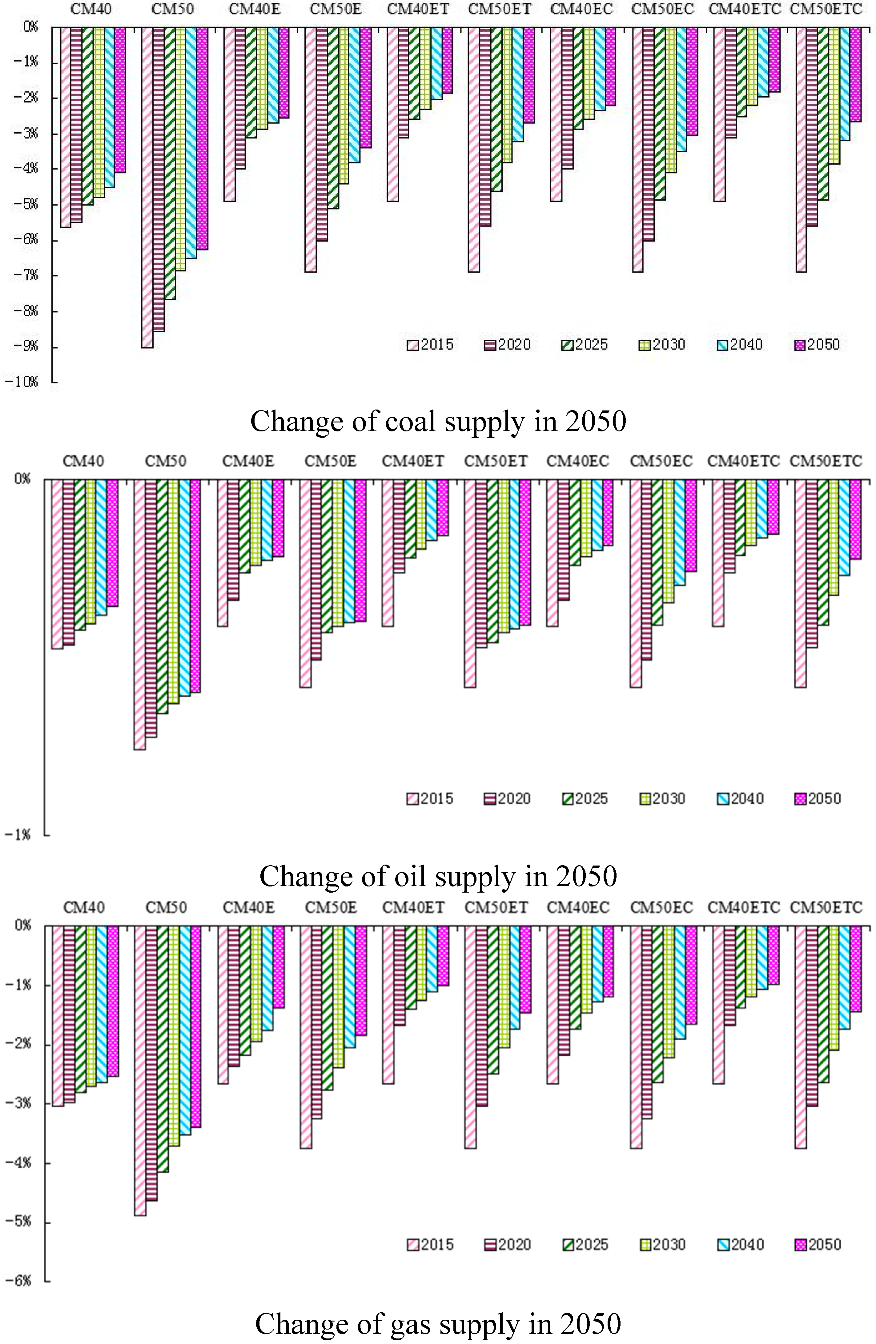
The impacts of carbon abatement on fossil energy supply in all the scenarios in 2050 are illustrated in
Figure 4. Despite the mitigation measures, coal supply by 2030 is expected to suffer a blow, which is due to the fact that coal combustion releases more CO
2 than other fossil energies.
Figure 4.
Change of fossil energy supply in the varied scenarios compared with BAU in 2050.
Figure 4.
Change of fossil energy supply in the varied scenarios compared with BAU in 2050.
Coal supply will be 3158 million tonnes coal equivalent (Mtce) in CM40ETC and 2960 Mtce in CM50ETC, accounting for 45.2% and 43.2% respectively in the total energy supply in 2050, while oil production will be almost unaffected,
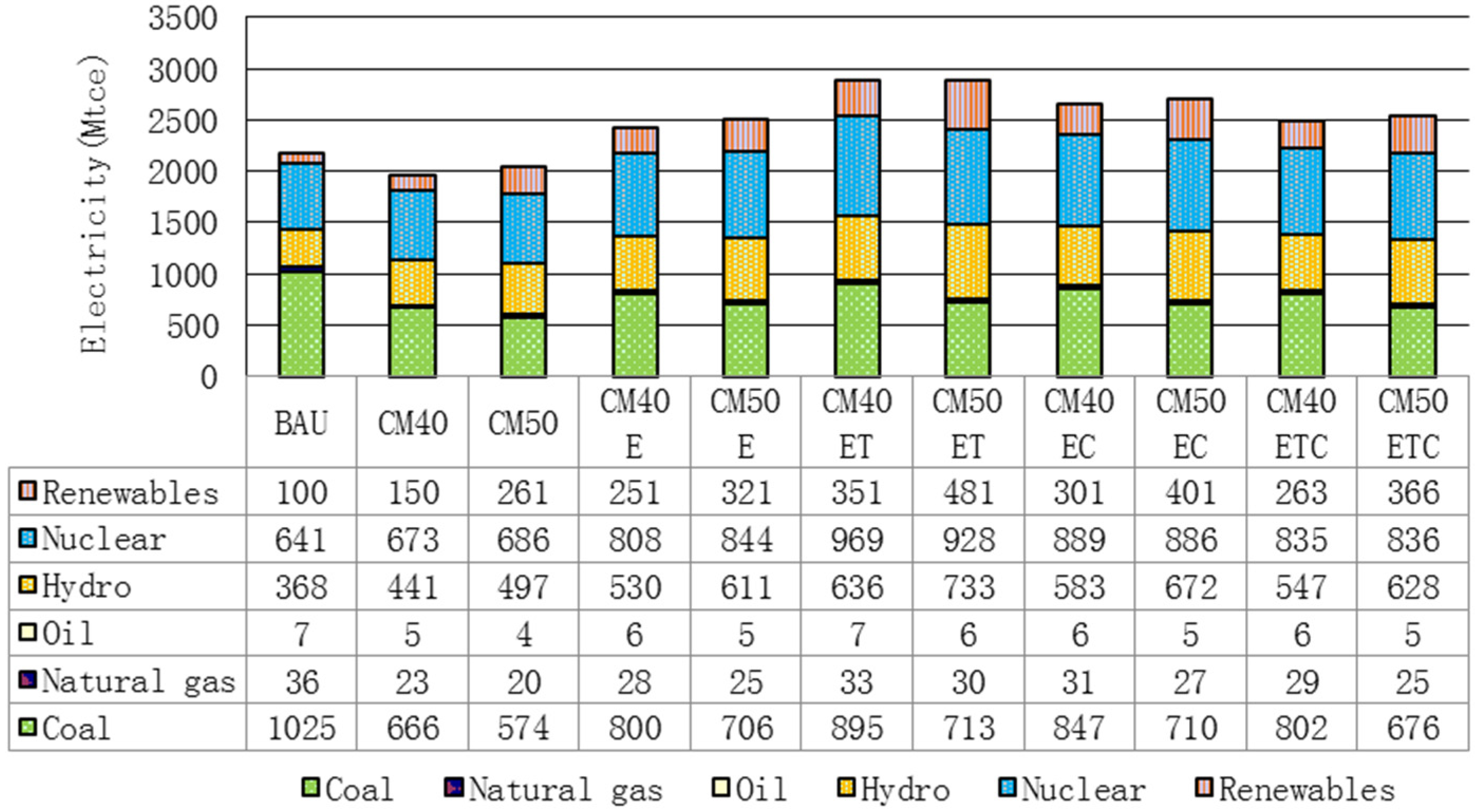
i.e., a slight drop of 0.78% in CM50, whose share will roughly remain unchanged in all scenarios. Limited resources and production capacities result in China’s heavy dependence on imported counterparts. The share of oil consumption remains steady, but oil consumption will severely depend on imports in 2050, with a degree of dependence of up to 80%, which is bound to increase energy security risks. China’s renewable energy development of wind, solar, and non-traditional biomass will replace fossil energy use. Meanwhile, renewable electricity generation increases significantly with the decreasing cost of renewable electricity. Renewable electricity in both the CM40 and CM50 scenarios sees relatively moderate increases, which indicates binding emission reduction commitments promote renewable electricity development to a certain extent (
Figure 5). Current emission reduction policies result in significant growth in renewable electricity generation. Furthermore, the total and renewable electricity in general are higher under the CO
2 emission reduction target of 50% than that at 40%. It is strongly noticeable that renewable electricity increases by approximately six times in CM50ET and the total electricity generation reaches 2584.52 Mtce, including 555.80 Mtce in thermal power, 730.02 Mtce in hydro power, 848.70 Mtce in nuclear power and 450.00 Mtce in renewable power, respectively. In contrast to CM40ET, the renewable energy contribution grows faster than that in CM40EC and the same situation occurs in CM50EC and CM50ET. In addition, the contributions of nuclear and hydro power in the scenarios with emission trading increase significantly that with a carbon tax. In comparison, emission trading is more efficient than a carbon tax in term of promote renewable energy development.
Figure 5.
The total electricity generation mix through 2050.
Figure 5.
The total electricity generation mix through 2050.
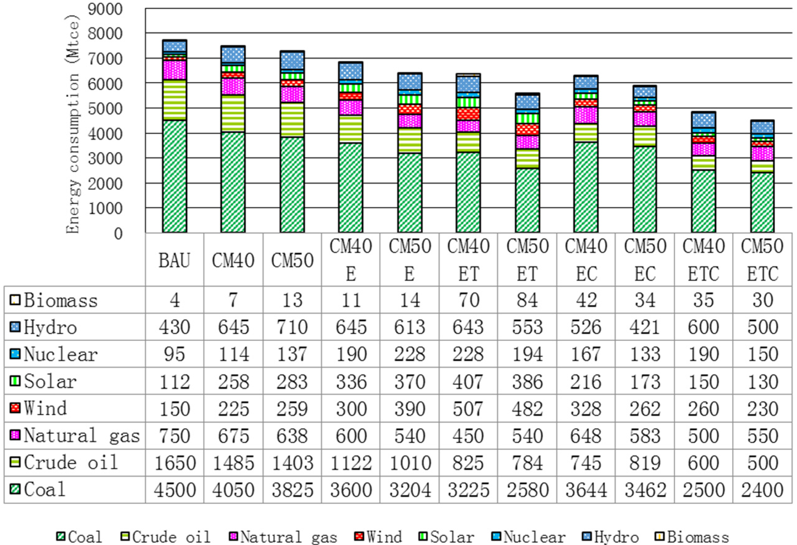
Figure 6 and
Figure 7 show the total primary energy consumption by sector and by type in 2050. Primary energy consumption decreases dramatically in all countermeasure scenarios. Compared with the BAU scenario, primary energy consumption sees a decrease of 3.01% and 5.50% in CM40 and CM50 respectively. A substantial fall in primary energy consumption is observed in the scenario with emission reduction measures, whose trend is more obvious when a higher emission reduction proportion is adopted. For instance, in the scenario, the renewable and emission trading and the primary energy consumption drop significantly by 17.35% in CM40ET, 37.12% in CM40ETC, 27.13% in CM50ET, and 41.61% in CM50ETC, respectively. Meanwhile, the total primary energy consumption reduces to 4835.20 Mtce in CM40ETC and 4490 Mtce in CM50ETC, in which the share of non-fossil energy is 29.19% and 32.33%, respectively. The primary energy structure in the CM40 and CM50 scenarios is not significantly different from that in the BAU scenario, implying that compulsory emission reduction measures do not improve the energy mix. The oil and natural gas consumption remain rather stable in CM40 and CM50, while the consumption in all countermeasure scenarios declines by 10%–40%. Coal consumption experiences dramatic decreases with the amount being 44.45% and 46.67% of BAU’s level in CM40ETC and CM50ETC. Cumulative energy savings is estimated to be 27,625 Mtce in CM50ETC and 15,301 Mtce in CM50ETC from 2020 to 2050.
Figure 6.
The total energy consumption by fuel types through 2050.
Figure 6.
The total energy consumption by fuel types through 2050.
Figure 7.
The total energy consumption by sector through 2050.
Figure 7.
The total energy consumption by sector through 2050.
In the countermeasure scenarios, the energy use in energy-intensive sectors declines significantly. It is visible that manufacturing, whose energy consumption decreases by 31.5% in CM40ETC and 35.2% in CM50ETC, respectively, is the highest energy consuming sector which suffers the greatest decline. The energy consumption in the service sector increases from 18%–34%.
3.6. Sensitivity Analysis
The sensitivity analysis of this AIM/CGE model should be tested to identify whether the result will be heavily influenced by parameter assumption. In this study, a sensitivity analysis is conducted with respect to the elasticities between the production factors labor and capital (), fossil energy and electricity (). We focus on the impacts of a 5% increase or drop from the base value on GDP and carbon intensity in CM40E and CM40ET.
Higher elasticity of means higher flexibility for producers to choose the factors of labor and capital when fulfilling their production quotas. Consequently, production cost drops away relatively, which results in higher activity levels and GDP growth. Results show that GDP loss is reduced by 4.36% from the base value. However, the carbon intensity do not change dramatically.
The have a significant impact on carbon intensity and GDP. A 5% increase of leads to a 11.49% drop of carbon intensity and a 5% drop of leads to a 6.38% increase. Higher put pressure on energy and carbon prices. Energy consumers have greater choice and flexibility to choose which kind of energy to consume. Hence, lower cost energy will be chosen, i.e., natural gas and electricity. The lower energy price stimulates production and drives GDP growth. Meanwhile, the carbon intensity will drop due to habit changes.
4. Conclusions
This study introduces the AIM/CGE model to investigate the effects of alternative mitigation policies, including renewable energy, emission trading and a carbon tax during 2010–2050. The simulation results show the effect on carbon intensity, activity level, GDP, energy system, and carbon prices in detail.
The emission reduction rate in the BAU scenario is approximately 28.68% in 2020 and 46.8% in 2050, based on the level of 2005. Absolute emission limits show negative impacts on future economic growth and activity level in energy intensive sectors. Activity level in non-energy intensive sectors increases slightly. In addition, the impact is larger when a higher emission reduction target level is set. In contrast, mitigation measures will curb CO2 emissions, promote economic growth and optimize the energy mix. More importantly, energy-intensive sectors will improve energy utilization technology as far as possible to lower their costs. The cumulative energy consumption reduction is estimated to be 27,625 Mtce in CM50ETC from 2020 to 2050. Moreover, climate policies lead to lower emissions, reduced energy intensity, and improved energy and industrial mixes. It is necessary to take all the measures into account to reduce emissions.
Among the mitigation measures, renewable energy makes a critical difference in abating emissions during the period from 2010 to 2020, reducing emissions per unit of GDP by 33.33% in CM40E and 36.43% in CM50E. After 2020, according to the hypotheses, abolishing subsidies on renewable energy will slow down the pace of development of renewable energy, which means that energy efficiency improved by renewable energy will affect the accompanying emission mitigation. Nevertheless, the renewable introduced reduces about 36% of the emissions per GDP, but still fails to meet the goals. Therefore, it is necessary to pay more attention to the development of renewable energy and the determination of the appropriate subsidy rates for renewable energy.
The emission trading introduced in 2016 will bring about high carbon prices, i.e., 143.4 USD/t in CM40ET, which encourages emissions reduction. Limited emission trading does not lower the carbon emission intensity as expected. Free emission trading must be integrated with mitigation measures to achieve the emission reduction targets. The government should try its best to plan the implementation of emission trading to avert unfair and unreasonable factors.
Carbon taxes would reduce carbon emissions, however, they does not work very well in the long term. Most noticeably, carbon taxes have a considerable negative impact on the sustainability, optimization of energy and economy system in the short term. It is necessary to give perfect rein to carbon tax by setting different tax rates.


