Implementation and Control of a Residential Electrothermal Microgrid Based on Renewable Energies, a Hybrid Storage System and Demand Side Management


Abstract
: This paper proposes an energy management strategy for a residential electrothermal microgrid, based on renewable energy sources. While grid connected, it makes use of a hybrid electrothermal storage system, formed by a battery and a hot water tank along with an electrical water heater as a controllable load, which make possible the energy management within the microgrid. The microgrid emulates the operation of a single family home with domestic hot water (DHW) consumption, a heating, ventilation and air conditioning (HVAC) system as well as the typical electric loads. An energy management strategy has been designed which optimizes the power exchanged with the grid profile in terms of peaks and fluctuations, in applications with high penetration levels of renewables. The proposed energy management strategy has been evaluated and validated experimentally in a full scale residential microgrid built in our Renewable Energy Laboratory, by means of continuous operation under real conditions. The results show that the combination of electric and thermal storage systems with controllable loads is a promising technology that could maximize the penetration level of renewable energies in the electric system.1. Introduction
Renewable energies bring numerous advantages to the energy matrix. They are inexhaustible at a human scale, non-polluting, provide energy independence and make possible distributed generation (DG), thus reducing transmission losses and increasing system overall efficiency [1,2]. However, an electric system with a high penetration level of renewable energies needs to overhaul its management techniques, due to the intermittent and distributed nature of renewable sources such as sun irradiation and wind speed [3,4].
So far, the deployment of wind and solar farms has been generally done within strong electric networks which are based on conventional generation. As such, the power injection into these grids from renewable generators has been done without restrictions. However, the continuous growth of renewable generators in the system is starting to worry grid operators to such an extent that in countries like South Africa or Germany, new regulations for grid connection of such systems are being created. These regulations specify the maximum fluctuations of the generated power in order to not disturb the grid as well as ancillary services such as primary frequency regulation, voltage regulation or ride-through specifications [5,6].
Likewise, the deployment of renewable energies within weak grids such as islands or remote rural areas, requires the participation of these sources in the grid regulation. As an example, in Puerto Rico, as well as in the aforementioned countries, there is a regulation for the connection of renewable energy generators into the grid which specifies the conditions for power injection into the system [7]. The compliance of these regulations often requires the use of storage systems, which will characterize the electric systems with high penetration levels of renewable energies. In [8], a country-scale analysis is performed with the purpose of calculating the minimum cost of an electric system with up to 99.9% of energy needs met with big renewable energy farms with the aid of different storage systems.
At a lower scale, renewable energy sources can be connected at low voltage consumption points within the main grid. This kind of DG, installed at consumption spots, with self-management abilities and tied to the grid at one only connection point, are the so called microgrids [9]. These microgrids would be the fundamental unit of a new distributed grid management system, and could be integrated in factories, office buildings, apartment buildings or, as proposed in this paper, in single-family houses. With the aid of appropriate storage technologies, they are able to control the power exchanged with the grid, participating in its management as the fundamental units of the smart grid. There are different storage technologies that can be used in microgrids such as batteries, flywheels, supercapacitors, etc. [10]. Due to the trade-off between power and energy densities, nowadays, the most used technology is based on electrochemical batteries, whether they are lead-acid or lithium-ion technologies. Such microgrids are able to work islanded in case of grid failure, thus assuring the power supply to the local loads at any time, improving the supply reliability. Nevertheless, batteries pose such an overcost to the microgrid that it is essential to optimize their use, that is, to achieve the grid connection specifications with the minimum battery size.
For the control of the power exchanged with the grid, the power reference can be given by a higher entity within the power grid (e.g., an aggregator) [11], or it can be calculated on site using live grid parameters (e.g., frequency, voltage, etc.) or finally, it can be calculated independently from the grid state. In this case, the microgrid can use its management ability to peak shave and smooth the power profile exchanged with the grid. This last option is important because of three points: (1) low voltage grids, usually designed for one direction power flows, can suffer overvoltage events when the power flows out from the microgrid, into the grid [12,13]; (2) the size of the distribution network can be significantly minimized when both consumption and generation power peaks are reduced or, in other words, electricity use can be increased without the need of a bigger electric network [14]; and (3) the reduction of power fluctuations helps stabilizing weak grids keeping its voltage and frequency values more constant and getting in the end better grid quality [15,16].
The energy management strategy is one of the key points when optimizing the profile of the power exchanged with the grid. The most intuitive approach for reducing power peaks and fluctuations is to apply a low-pass filter to the net power within the microgrid, i.e., the difference between power consumption and generation [17,18]. This strategy would consist on separating the components of the net power by means of applying a moving average, thus getting a high frequency component that would be assumed by the batteries and a low frequency component that would be exchanged with the grid. However, the biggest disadvantage of such a strategy is that the filter is applied independently of the state of the system, without considering variables such as the state of charge (SOC, percentage over the useful value) of the batteries thus under-using the storage system or, in other words, forcing to over-size it to attain certain power profile requirements.
In [19], a more sophisticated strategy is proposed which consists in a series of steps that seeks to optimize the storage element, while flattening the power profile exchanged with the grid. In order to do so, a weighed share-out of the net power is carried out between the grid and the batteries, using coefficients depending on the SOC of the batteries. This same management philosophy is used in [20], implemented in this case using fuzzy logic. These strategies manage to attenuate power peaks and fluctuations at the point of common couple (PCC), but are still unable to use the full potential of the batteries. For instance, during periods of time when the energy generated exceed the energy consumed, the useful SOC of the battery moves around 75%, between 50% and 100% values, precisely when one would like to have the battery partly discharged in order to absorb the excess of generation. Likewise, during periods of time with more consumption than generation, the battery useful SOC moves around 25%, between 0% and 50%, when the batteries should be more than half charged in order to compensate the lack of generation. This seasonal behavior means that the battery capacity is not being entirely used when looking at daily intervals, and as a result, the battery potential is not being fully used for peak shaving and smoothing the power profile at the PCC.
Besides, the system performance can be improved if the electric system is coupled with the home thermal energy system, resulting in a thermo-electric microgrid. The thermal system in the house can improve management capabilities as well as provide cheap and easy to implement energy storage. For instance, the thermal deposits already existing in the house can be used as a complementary energy storage system, like hot water tanks, or the building's thermal energy itself [21].
Additionally, the demand side management (DSM) techniques, that permit the control of certain deferrable loads, decrease the needs for storage capacity, by connecting such loads when the renewable energy is being generated. Some authors [22,23] give the grid operator permission to control certain loads, like air conditioning systems, to help peak shaving the power demand. Another proposed approach [24–26] is the use of dynamic pricing systems, accessible for the user, who can set certain devices like dish-washers or washing machines to work at off-peak hours. Yet another possibility, in line with the idea of using existing elements in the system, is the use of an electric water heater that thanks to an added electronic converter can be used as a controllable load. In this way, the power consumed by the heater can be controlled automatically and in real time by the energy management system (EMS) in an easy way and with a rapid response.
In this paper, we propose an energy management strategy based on that explained in [19,20] for an electro-thermal microgrid based on renewable generation, hybrid electro-thermal storage system and a controllable water heater whose consumption can be deferred thanks to an attached hot water tank that acts as an energy buffer. The water heater is considered as the best choice to be used as a controllable load because while being a high power device, it can consume whichever power from zero to its rated power with a rapid response. Moreover, as long as the water tank temperature is maintained within its operating range, the management of the water heater will not affect the user in a negative way, unlike the air conditioning system control.
The designed energy management is in charge of determining at every moment the power reference for the water heater and the battery, depending on the SOC, the water tank temperature, and the energetic state of the microgrid, with the objective of peak shaving and smoothing the power profile exchanged with the grid. One of the key differences when compared to [19,20] is that by considering seasonal fluctuations in both generation and consumption power profiles, the energy management strategy can now maintain the SOC around 50% during the whole year, but allowing for daily variations ranging the 100% of the SOC. In this way, the battery use is maximized, allowing for the maximum attenuation of the power profile exchanged with the grid. In addition, the thermal system has been linked to the electric microgrid, creating the electro-thermal microgrid which provides extra energy storage and a controllable load which allows us to enhance the results.
The strategy has been experimentally validated in the Renewable Energy Laboratory at Public University of Navarre (UPNa), in a configurable energy system that allows setting up different microgrids, and which is set up in this case as a single family home, equipped with the aforementioned managing units, in charge of controlling the fluctuating renewable energy generation as well as the house consumption.
In Section 2, the setup of the microgrid is defined and a base scenario is analyzed. In Section 3, a first approach using a low-pass filter based strategy is introduced, which is later enhanced in Section 4 with the proposed management strategy. Regarding the experimental validation, the microgrid deployed in the Renewable Energy Laboratory at the UPNa is described in Section 5, along with the results obtained. Finally, in Section 6, the conclusions are discussed.
2. Analyzed Microgrid: Characteristics and Power Profile at the PCC without an EMS
2.1. Description of the Microgrid
The principles of the energy management strategy presented in this paper are valid for any microgrid based in renewable generation and a hybrid storage system. However, for its validation, the case study has been particularized for a single-family home microgrid. Hence, all the results presented in this paper refer to such a configuration, which is described in detail in this section.
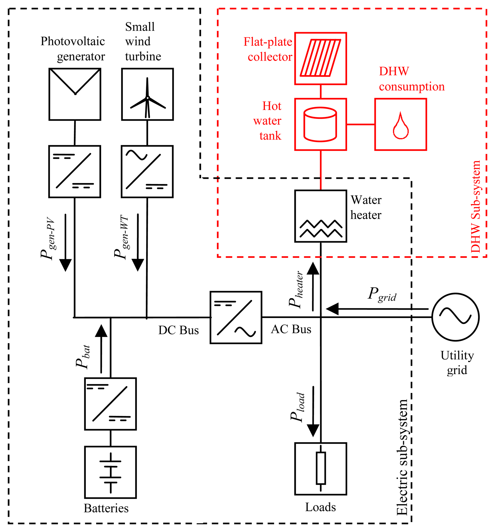
The home's energy demand consists of the typical electrical loads (lighting, electrical appliances, etc.), space heating and cooling and domestic hot water (DHW) consumption. Hence, two energy subsystems necessarily coexist, an electrical one and a thermal one, which comprise, apart from the consumption elements, generation and storage subsystems.
The electric subsystem, apart from the aforementioned loads, comprises a photovoltaic (PV) array of 4 kWp and a small wind turbine with a rated power of 6 kW. The storage system includes a lead-acid battery with a total capacity of 72 kW h. The life of this type of battery is significantly reduced when operated at high depth of discharge (DOD) levels. For this reason, it is recommended to operate lead-acid batteries at a maximum DOD of 60%–90% [27]. In order not to compromise the life of the batteries, a maximum DOD of about 60% has been chosen, which in this case means that the useful capacity of the battery is 45 kW h.
Considering that the energy management strategies are designed in a way that makes the SOC to move around 50% of its useful capacity, it can be said that the battery offers about ±15 h of the mean electric demand of the house, which is 1.5 kW. Hence, this battery capacity is thought to be enough to attenuate up to daily power fluctuations provided that the right energy management strategy is applied.
The thermal subsystem is in charge of providing DHW and space heating and cooling. The latter is provided by a heating, ventilation and air conditioning (HVAC) system rated 5 kW which works as a passive load, i.e., not controlled by the EMS. Regarding the DHW system, it comprises an electric water heater (4.5 kW), a flat-plate collector array (2 kW) and an 800 L hot water tank that allows storage of up to 50 kW h, depending on the range of temperatures allowed.
From the energy management point of view, there are two energy systems that are in principle separated, the electric system and the DHW system. Both systems are connected via the water heater, resulting in one only energy system, called electro-thermal microgrid (see Figure 1). Furthermore, the water heater is a key element of the energy management as, being a controllable load, provides an extra degree of freedom when controlling the power exchanged with the grid.
The electric consumption data used for the simulations has been directly measured from the mains of a house, using a power analyzer registering data every 15 min during over a year. The DHW consumption has been taken from a typical profile for a single-family home. The microgrid is designed so 70% of the energy demand is met with on-site renewable energies, meaning that, while working in normal operation, that is, grid connected, the electric utility would provide the remaining 30%. The energy generation has been calculated using irradiance, wind speed and temperature data from the microgrid site (Pamplona, Spain: 42°49′06″N 1°38′39″O) collected by the weather station at UPNa.
In this configuration, the instant electric power balance within the microgrid can be achieved with different combinations of the power of the battery, the water heater and the grid. In this way, controlling the power of the battery and the water heater, the power exchanged with the grid can be controlled. The Equations (1)–(3) are obtained from Figure 1:
| Pgrid | Power delivered by the grid; |
| Pbat | Power delivered by the battery; |
| Pheater | Power consumed by the electric water heater; |
| Pnet | Difference between the power consumed and the power generated; |
| Pload | Power consumed by the passive loads (i.e., not counting the electric water heater); |
| Pgen | Power delivered by the PV array and the small wind turbine; |
| Pgen_PV | Power delivered by the PV array; |
| Pgen_WT | Power delivered by the small wind turbine. |
2.2. Power Profile Exchanged with the Grid without EMS
In order to compare the results obtained using different strategies, a reference scenario is designed, in which there are no batteries and the water heater performs as a passive load that uses a hysteresis control of the temperature in the water tank between 60 °C and 80 °C, regardless of the rest of variables of the microgrid.
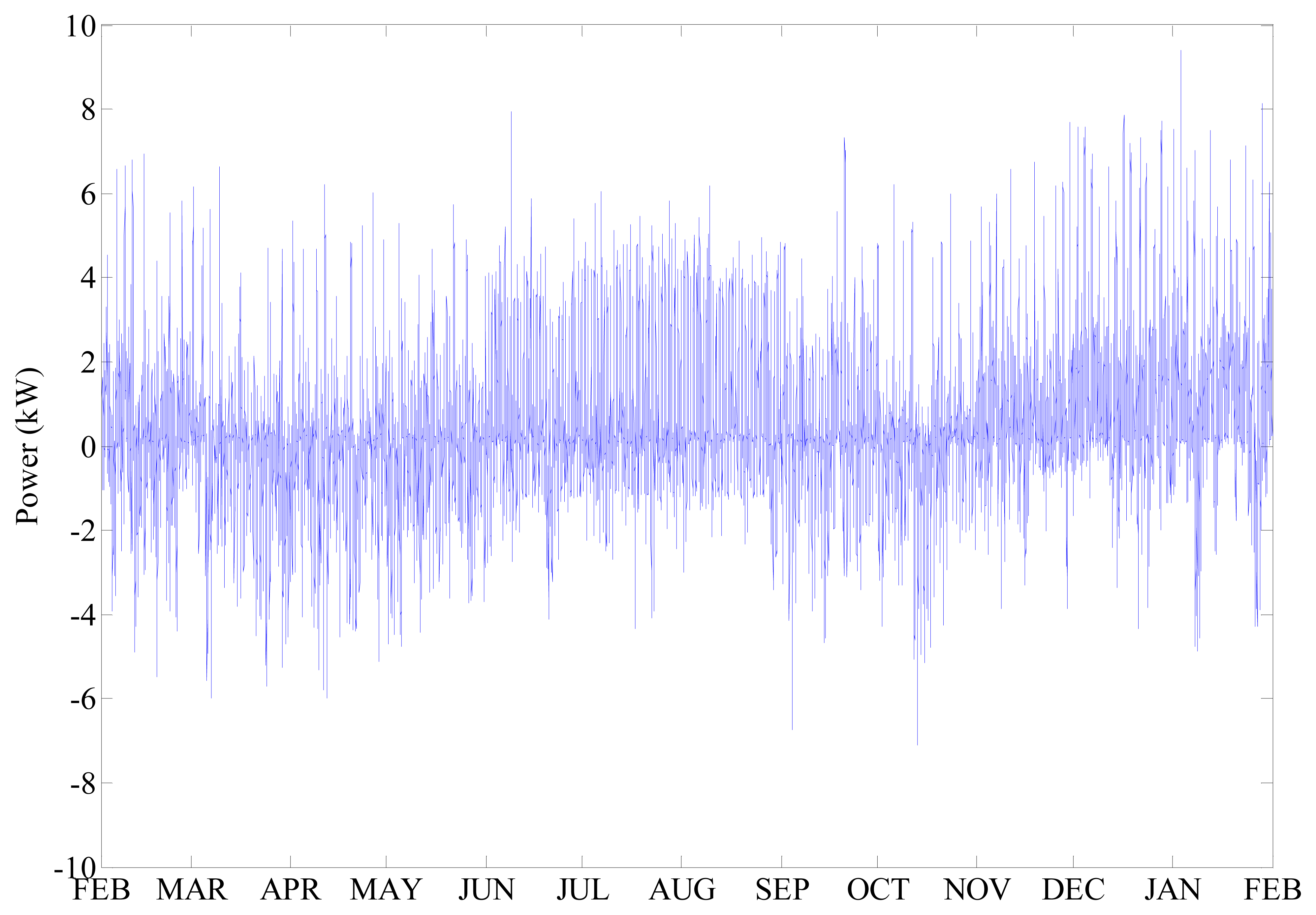
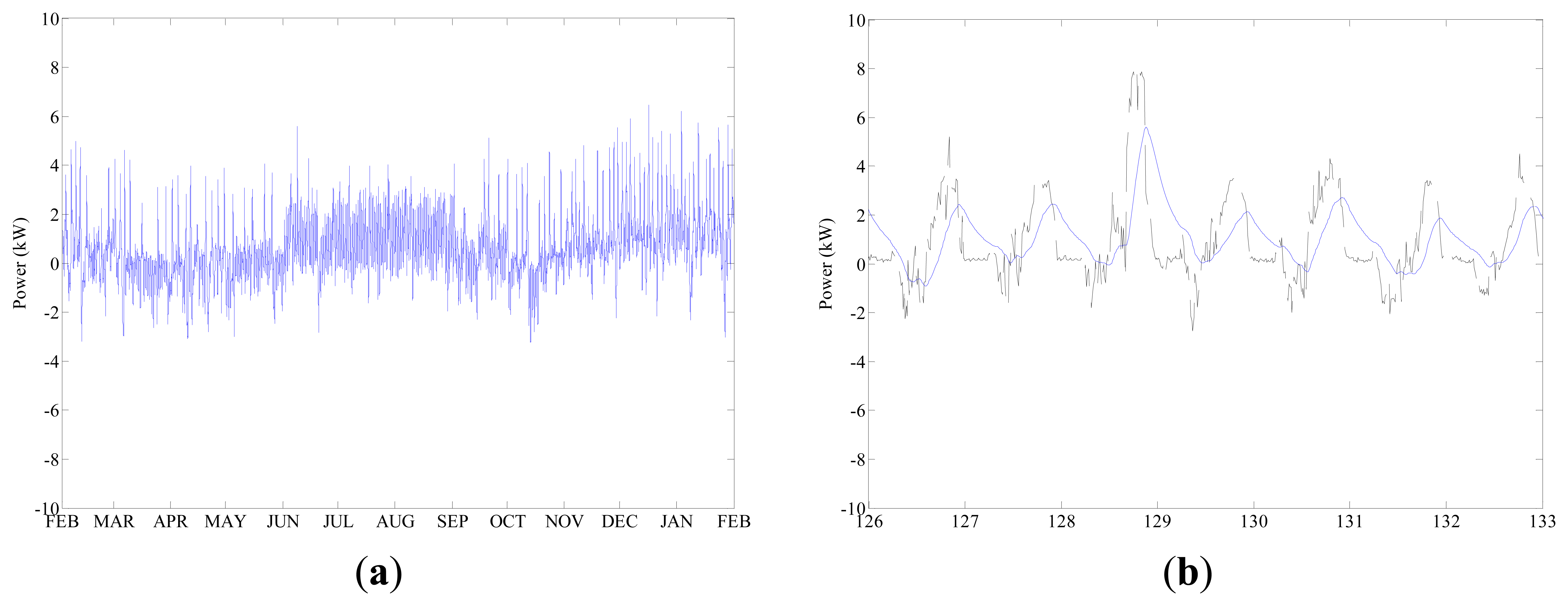
In this case, in the absence of any management elements, the value of the power exchanged with the grid is only determined by the power balance of the generators and the passive loads (Pnet); hence, the grid will suffer all the power peaks and fluctuations that these elements may cause. In Figure 2, the power profile of Pnet from February 2012 to February 2013 in 15 min intervals is shown.
As can be appreciated in Figure 2, the power profile of Pnet features high variability and has peaks of up to 9 kW for a mean power of 0.47 kW which in turn, would require the user to contract a power capacity much higher than its average consumption and would unnecessarily overload the distribution lines. Furthermore, these fluctuations, which range from positive values (consumption from the grid) to negative values (power fed into the grid), would carry negative consequences in a low voltage network in scenarios with high penetration levels of renewables.
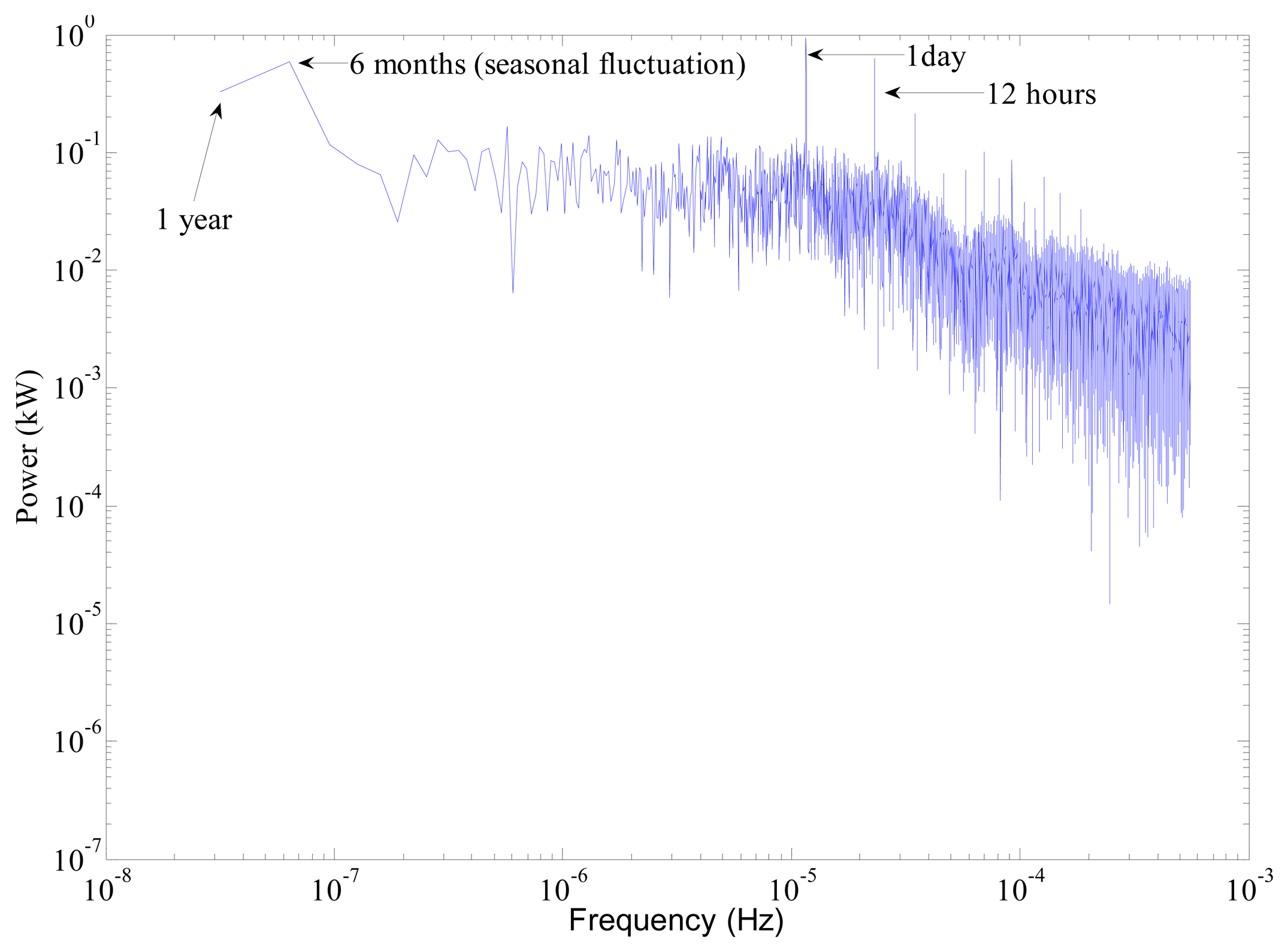
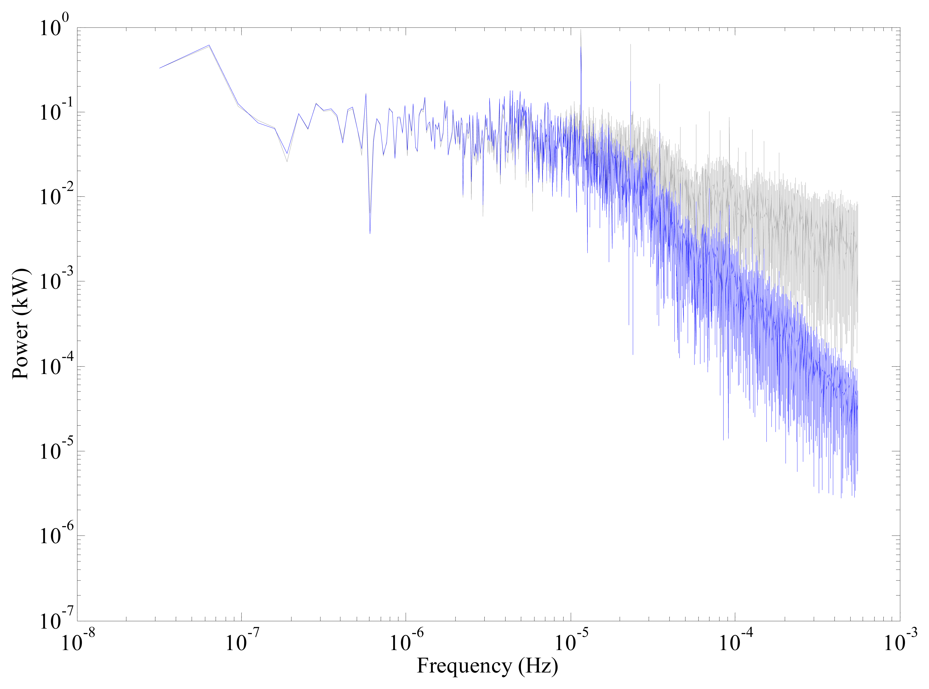
In order to analyze the fluctuations of the power profile shown in Figure 2, the spectrum analysis shown in Figure 3 is carried out. This analysis shows a strong yearly component mostly due to PV generation, that has its maximum daily production in the summer and its minimum in the winter. The next noticeable component is the seasonal one, which is caused mainly by the use of the HVAC system, whose consumption reaches maximum levels during summer and winter, while it is minimum in spring and fall. At a higher frequency, it is located the highest component, the daily one, which is partly due to wind generation but specially due to the variation of the consumption and PV generation which reach their maximum levels during the day and minimum during the night. There can also be found multiples of the daily components, due to renewable generation as well as consumption. Likewise, at higher frequencies there can be seen the rest of components due to both renewable generation and consumption.
3. Simple Moving Average Strategy
3.1. Definition of the EMS Strategy and Implementation
For peak shaving and for reducing fluctuations in a given power profile, in this case Pnet, the most intuitive strategy to use would consist of applying a low-pass filter to the power profile, in a way that the high frequencies were separated from the low ones. The high frequency components would be assigned to the battery, therefore, the grid would only have to exchange power at low frequencies. In this way, the grid would only see a smooth power profile, while the battery would compensate the rapid fluctuations in the net power as well as its peaks.
Given that the battery used in the proposed microgrid has a capacity of ±15 h of storage in relation to the average consumption, it does not make much sense to think that seasonal and yearly attenuations could be compensated, in which case the battery capacity would have to be much bigger. However, with this battery one should be able to attenuate the daily component, which is the one with the higher amplitude, as seen on Figure 3, as well as all the components of higher frequencies. With the objective of canceling this component, along with its multiples, the low-pass filter used consists of a 24 h window, simple moving average.
If all the power flows existing in the system were considered and exactly measured, the battery would exchange a power profile with a zero average value, and so its SOC would not change in the very long term. However, the losses at the battery cause that, without any additional control, the grid does not supply all the true energy needs of the microgrid, depleting the storage system. As a result, it is necessary to add a closed loop control of the SOC of the battery to compensate any deviation from its reference value. In principle, this reference value is set at 50%, with the objective of having as much energy exchange capacity in both directions.
The strategy is composed by two steps whose equations are explained below:
- Step 1:
In the first step, the high frequency components are separated from the low ones according to Equations (4) and (5) using a simple moving average with a window size of 24 h, which will eliminate daily fluctuations from the low frequency power profile:
where N is the number of samples in 24 h.- Step 2:
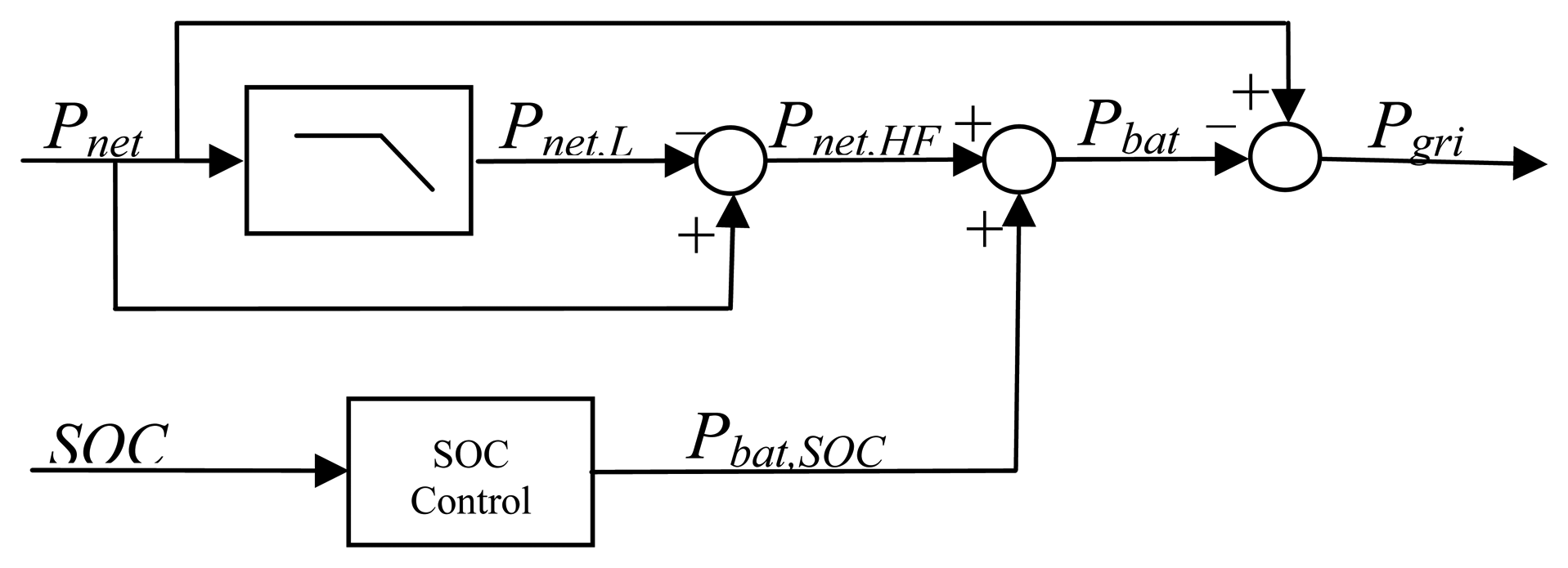
In order to keep the SOC of the battery around its reference value (refSOC = 50%) and within its limits, a proportional control is carried out, in accord with Equation (6), with a control constant K. The power assigned to the battery (Pbat) is the result of adding to the high frequency components of the net power (Pnet,HF), the power needed for the SOC control (Pbat,SOC). The power exchanged with the grid (Pgrid) is the difference between the net power (Pnet) and that assigned to the battery (Pbat):
To calculate the value of the control constant K, it should be considered that it must be big enough in order to keep the battery within its SOC limits, but as small as possible so the SOC fluctuations are not transferred to the grid power profile. This constant is minimized by simulating the performance of the system during a year using different values of K, and choosing the value which minimizes the quality criteria without exceeding the SOC limits of the battery, being 8.8 for the case study.
Figure 4 shows the block diagram of the whole strategy.
3.2. Simulation Results
Figure 5a shows the power profile at the PCC during a year. It can be clearly observed how the power peaks are reduced with respect to Pnet (shown in Figure 2). The reduction of the maximum power peak absorbed from the grid is 32.4%, and in the case of the maximum peak injected to the grid is 54.6%. Figure 5b shows a one week detail of this power profile (in blue), along with the net power profile (dashed line), making more visible the high frequency components' attenuation as well as the delay, due to the low-pass filter. However, it can be seen how daily fluctuations are still present in the power profile exchanged with the grid.
These fluctuations are due to the proportional control of the SOC, that introduces all the fluctuations of the SOC (seen on Figure 6), through the control constant, K. These oscillations could be attenuated using a smaller control constant K, however, choosing a lower K, implies that the low-pass filter window would need to be smaller as well, in order to keep the SOC within its limits. As a consequence, the daily fluctuations would not be eliminated in the first step. This observation leads to the realization that, by using this strategy, daily fluctuations cannot be totally eliminated but with the use of a larger battery.
Figure 7 shows the frequency spectrum of the power profile exchanged with the grid without applying any strategy (grey) and once the strategy is applied (blue). It shows how components with a frequency above the daily one, are strongly attenuated with respect to that of the net power profile (Pnet). However, it can be noticed how the daily component has been hardly attenuated.
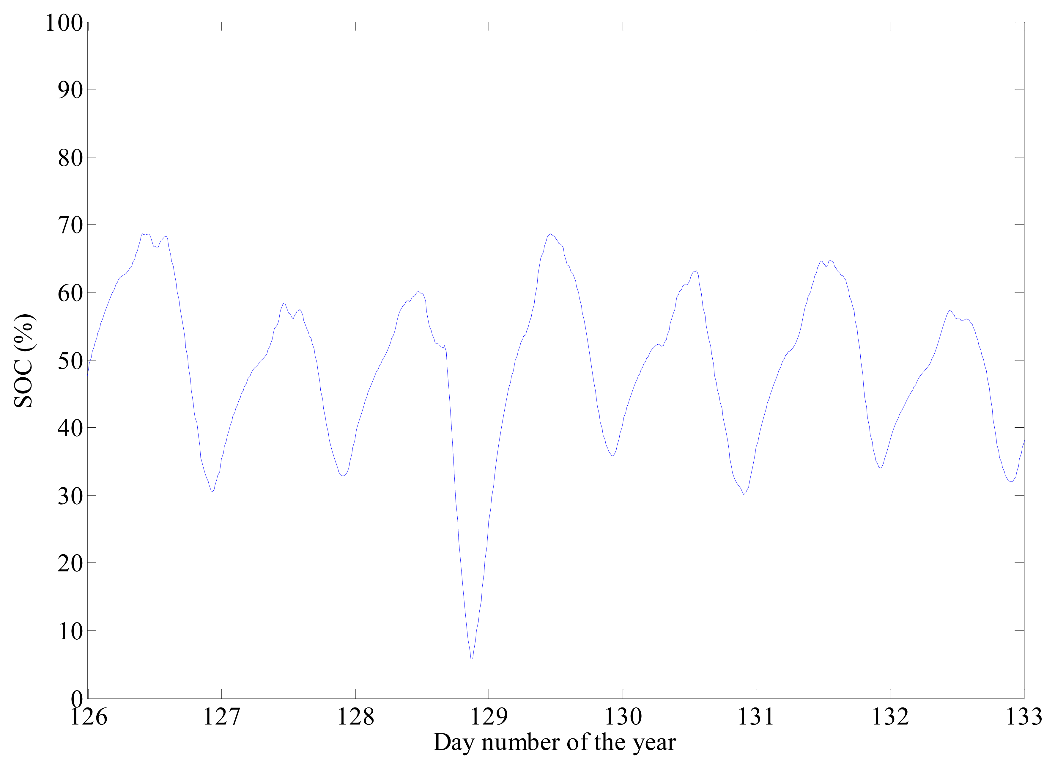
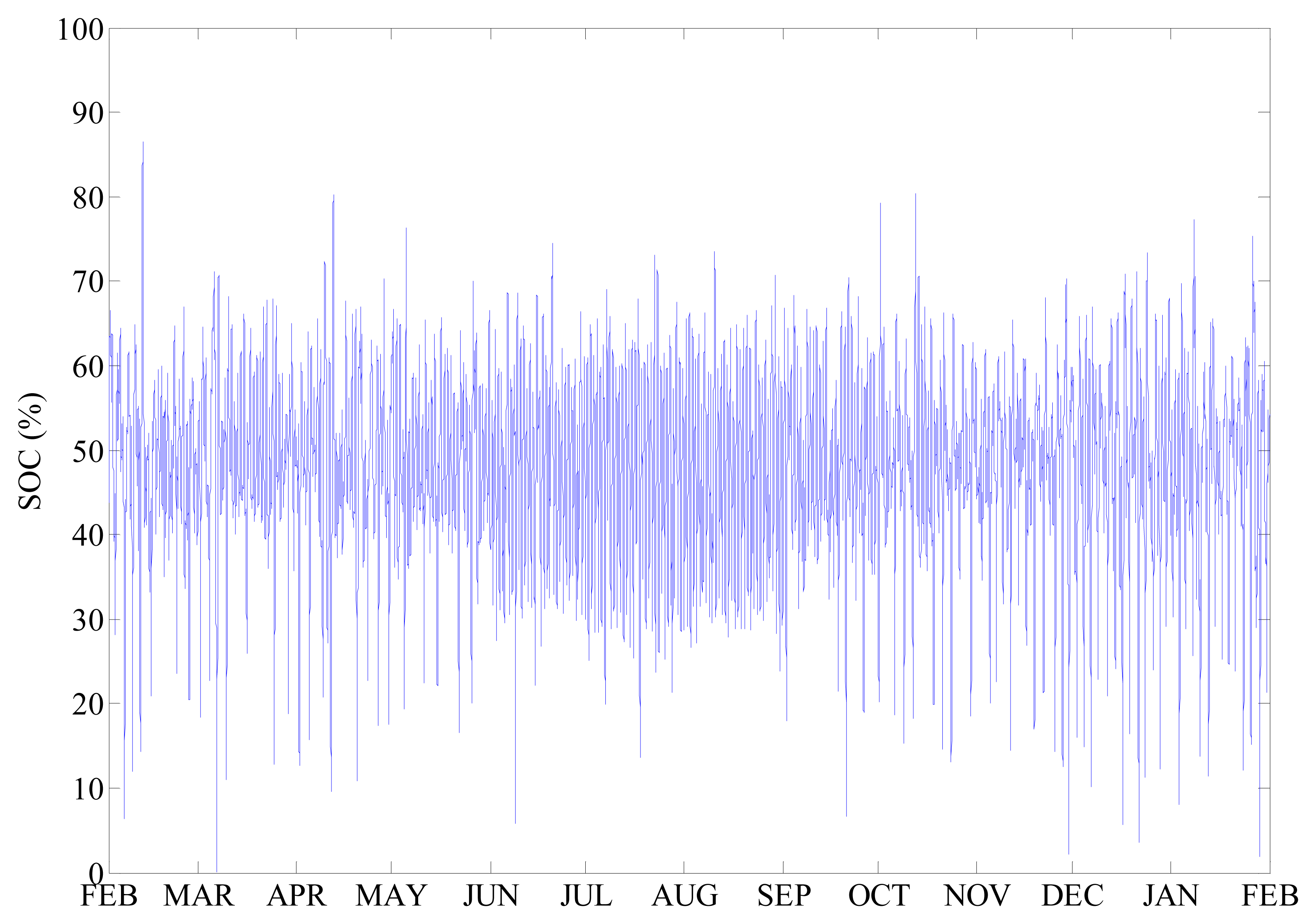
Additionally, Figure 8 shows the SOC evolution during the same year, where it can be observed how the batteries are being underused. This is because the SOC control is carried out regardless the rest of variables in the system, and so the control constant K has to be chosen so the SOC lies between its limits in the worst case. This occurs on 7 March, the day in which both the SOC of the battery and the temperature of the water tank are at low levels. In this situation, the hysteresis control of the hot water tank turns on the heater, totally discharging the battery. However, this situation does not occur many times in the year, which means that most of the time the SOC zone between 0% and 25% will remain unused.
Similarly, Figure 8 shows that the zone of the SOC between 75% and 100% is hardly used. This is mainly due to the power profile shape of Pnet, which tends to discharge the battery. This is explained by understanding the hysteresis control of the hot water tank, which turns on the heater at its rated power instantly, and keeps this power consumption for about 5 h. This behavior causes the SOC to fall suddenly, as seen in Figure 9. This understanding shows that using the water heater as a controllable load would highly improve the system performance.
4. Proposed Energy Management Strategy
4.1. Definition of the EMS Strategy and Implementation
The low-pass strategy certainly achieves some improvement with respect to the net power profile regarding power peaks and fluctuations attenuation. However, as mentioned before, the daily fluctuations are barely reduced, due in part to the under utilization of the battery. By designing a more intelligent energy management strategy that considers the state of all the different elements of the microgrid, a more exhaustive use of the battery would be achieved, and as a consequence, a better power profile would be exchanged with the grid. As such, the proposed strategy comprises a series of steps that seek to minimize the interaction with the grid, having into account the SOC of the battery, the temperature of the hot water tank as well as the power balance within the microgrid.
Furthermore, as an aid to the control of the power exchanged with the grid, the thermal system already existing in the house is used. By converting the electric water heater into a controllable one and by allowing a wider temperature range in the hot water tank, an extra degree of freedom is obtained that will be used to absorb the peaks of power generation, and to control the SOC of the battery, while keeping the temperature in the water tank within its limits.
The strategy designed consists of four sequential steps called S1, S2, S2_t and S3, as seen in Figure 10.
These steps, which are an evolution of the strategy seen in [19], are detailed below:
- (a)
Step S1:
The objective of this first step is to do a preliminary allocation of the net power between the grid and the battery, depending on the SOC of the latter. For instance, if the net power balance is positive, i.e., there is more consumption than generation, and the SOC is high, then all the extra power needed would be delivered by the battery. For a lower SOC, the power deficit would be shared out by the grid and the battery depending on the SOC. Finally, if the battery tends to 0% SOC, the grid will tend to supply all the energy needed. In case of having a generating balance, the logic applied would be the opposite.
In order to do this allocation, the power consumed (Pcon) and generated (Pgen) are measured in order to obtain P′net, which is the difference in Equation (9). Unlike the previous strategy, in this balance the power of the water heater is not taken into account as in this case, it is considered as a controllable load and its power reference is calculated afterwards:
The value of P′net, that can be positive (consuming balance) or negative (generating balance) is assumed by the grid and the battery in a proportion that depends on the SOC of the battery. The function that determines this proportion is different depending on whether the net power balance is positive (Kpp function) or negative (Kpn function). Thus, the power assigned to the grid and to the battery in this first step is calculated according to the Equations (10) and (11):
Kpp and Kpn, defined for all the battery SOC range, are calculated by Equations (12) and (13):where rx defines the point at which the function reaches the unity value, that is, the point at which the power is fully compensated by the battery. Note that the functions Kpp and Kpn are symmetrical in relation to the 50% SOC value. The optimal value of rx obtained for the particular case of this microgrid is 60, as it can be seen in Figure 11. Therefore, for example, if the net power balance is positive while the SOC is above 60%, all the power (P′net) will be provided by the battery. If the balance is still positive but the SOC was 20%, the battery would supply only 50% of P′net and the other half would be supplied by the grid.- (b)
Step S2. A preliminary design
The purpose of the second step, is to use the grid to bring the battery SOC close to the reference value of 50%, but only whenever the power assigned to the grid in the previous step (Pgrid,S1) is within the limits ±Plim, so to limit the power demanded to the grid. Whenever Pgrid,S1 is within these limits, and the SOC is above 50%, the power value assigned to the grid is decreased to −Plim so the battery is discharged. In the case of the battery SOC being below 50% the power assigned to the grid would be +Plim, in order to charge the battery. With the purpose of avoiding sudden shifts in the reference value of Pgrid, a ramp function is used to link the values of ±Plim smoothly as seen in Figure 12, where the value of P2 is represented as a function of the SOC, and corresponds to Equation (14):
where Plim (kW) is the limit power value; rr1 and rr2 (%) are the values which define the ramp function.This preliminary design of Step S2, will not bring the expected results, but is important to understand why, in order to understand its final design, which will be explained under Section 4.4. As such, the results of the strategy using this preliminary design are firstly explained.
The rules for obtaining the value of the power assigned to the grid in the second step are defined in Equations (15) and (16):
To explain this graphically, whenever the power assigned to the grid in the previous step (Pgrid,S1) falls into the grey zone for a given SOC, the new value assigned to the grid (Pgrid,S2) will be P2. In case of Pgrid,S1 falling out of the grey zone, the value assigned to the grid in step 1 prevails.
The value of Plim has to be as low as possible, to avoid overloading the grid and to reduce fluctuations in the power profile, but also, it has to be large enough to be able to control the SOC of the battery. In the microgrid analyzed, the optimal value obtained, shown in Figure 12, is 1.2 kW, equivalent to 2.5 times the mean value of the net power.
- (c)
Step S2_t
In Step S2_t, the power assigned to the heater is calculated with three main goals:
Control of the water tank temperature;
Reduction of the power peaks injected into the grid;
Additional control of the battery;
With this purpose, the power assigned to the heater will be dependent on the water tank temperature, the SOC of the battery and the power balance in the microgrid. The total power assigned to the water heater is calculated in two sequential stages. In the first one, the power coming from the grid is determined, and in the second one, the power coming from the battery.
As it can be observed in Figure 13, the power reference calculated for the heater in the first stage, depends on the temperature in the water tank and on the power assigned to the grid in the previous step (Pgrid,S2). In the first place, and to avoid the temperature in the tank to surpass the temperature limits, the power reference of the heater is set to its rated power in case of being under the minimum temperature limit, and it is set to zero whenever the water temperature overpasses the maximum limit.
Within the limits of temperature, there are three operating zones, depending on the value of the power assigned to the grid on Step S2. The first operating zone is the one in which Pgrid,S2 lies above a certain limit of power absorbed from the grid. In this zone the power reference for the heater is set to zero. The power limit that defines this zone is normally equal to the power limit seen in S2, i.e., Plim. However, when the temperature in the water tank falls below 50 °C, this power limit will be increased by a factor of Kxy, which allows to consume power from the grid up to two times the power limit Plim, gradually and depending on the water temperature, accordingly to the curve in Figure 14.
The second zone corresponds to a value of Pgrid,S2 between the maximum power absorbed from the grid limit, Kxy·Plim, and the maximum power injected in the grid, limG. In this case, and always within the temperature limits, a gradual temperature control is carried out, that depends on the aforementioned coefficient Kxy, and a new coefficient Ktt. This coefficient's purpose is to prevent the heater to be turned on whenever the temperature is above the reference temperature (Figure 14). Moreover, the variation of this coefficient is gradual and dependent on the temperature in order to avoid introducing fluctuations in the power exchanged with the grid.
The third zone corresponds to the case in which Pgrid,S2 falls below the negative limit (limG), in which case the heater will absorb the difference between these two values. As such, the power injected into the grid should never be greater than the limit set, limG. The lower is the absolute value of limG, the more are reduced the power peaks injected into the grid. However, if this value is too low, too much power would be assigned to the heater, and during bigger time intervals. This would make the temperature of the water tank to reach the maximum value, and the degree of freedom would be lost. The compromise value for limG for this microgrid is −0.9 kW.
Equations (17)–(21) are used to calculate the power assigned to the heater in this first stage of its control:
The power assigned to the water heater in this stage, modifies the power assigned to the grid, as such, the new power reference of the grid is calculated according to Equation (22):
In the second stage of the heater control, whenever the temperature is under the maximum limit, the heater will be used to transfer energy from the battery to the water tank, if the battery SOC is above 96%. In this way, the difference between the rated power of the heater and the power assigned to the heater in the previous stage is used to discharge the battery so to recover the ability of the battery to absorb energy. Equations (23) and (24) are used to calculate the value of power added to the heater, Pheater,2, in this second stage of the control of the heater:
This component only affects to the power finally assigned to the heater, and to the battery. The new power values of these two elements are calculated according to Equations (25) and (26):
- (d)
Step S3
The goal of this last step of the energy management strategy is to eliminate the high frequency components that may remain in the power assigned to the grid. With this purpose, a simple moving average low-pass filter (with a 2-h window in this case) is applied to the power assigned to the grid at the end of the previous step (Pgrid,S2_t). The high frequency band (Pgrid,S2_t,HF) is assumed by the battery while the low frequency band (Pgrid,S2_t,LF) is assigned to the grid:
In this way, the power finally assigned to the battery is calculated according to Equation (28):
4.2. Simulation Results for the Preliminary Strategy
Figure 15a shows the power profile at the PCC for the same period of time shown in Figure 2. Comparing this profile with the one obtained by applying the simple moving average strategy (Figure 5a) it can be noticed that the maximum and minimum values of the power exchanged with the grid have been strongly reduced. In fact, during most of the time, the power exchanged with the grid is limited to values between limG and Plim, (−0.9 kW and 1.2 kW. respectively).
However, in Figure 15a it can be observed how during summer and winter months, the value of Plim is overpassed many times. This is caused by the fact that during these months there is more consumption than generation (due mainly to the space heating and cooling) and as a result, during these months the SOC of the battery oscillates around 30%, as observed in Figure 15b, where the SOC evolution during a year is shown. This fact, limits the ability of the battery to provide the extra consumption of the microgrid which in turn makes the share of the grid to be bigger. Similarly, it is observed that the SOC tends to high levels during spring and fall, when the generation is higher than the consumption. In these cases, however, the power exchanged with the grid does not overpass the limit of power injected into the grid (−Plim) because the heater copes with the negative power peaks, and finally limits the actual value of power injected into the grid.
4.3. Enhanced Step S2 and Final Proposed Strategy
As previously seen, the results of the preliminary strategy are limited by the evolution of the SOC during a year due to its dependence with P′net. In order to avoid such a dependence and to get better results, a modification is proposed with the objective of making the SOC fluctuate around 50% independently of the value of P′net. To correct this dependence of the SOC with P′net, a set of three modifications are proposed to step S2, which is precisely the one in charge of controlling the SOC value.
In the first place, it is proposed that the SOC reference value varies in relation to the energy balance inside the microgrid in the last 24 h, that is, the daily average of P′net, noted P′net,avg. The objective is to tend to charge the battery if there has been more consumption than generation during the last 24 h, and to tend to discharge the battery if the energy balance has been negative. With this purpose, the SOC reference, refSOC, which previously was constant and equal to 50% (as seen in Figure 12), is now defined as a variable dependent on P′net,avg. This linear function is saturated at certain values of P′net,avg which are noted ±limit. In the case of this microgrid, this limit is set to ±1 kW, bounding the value of refSOC to 10% and 90%, as seen in Figure 16.
In this way, refSOC, is calculated by means of Equation (29):
Secondly, as seen in Figure 2, there is an asymmetry in the net power profile in terms of both energy, as the annual energy balance is positive, and power, as the power peaks are bigger when positive (consumption) than when negative (generation). Furthermore, the heater absorbs the negative peaks, increasing the asymmetry. Therefore, it becomes clear that the positive and negative limits for power peaks in the power profile (+Plim and −Plim) have to be decoupled, and their new values will depend on the characteristics of the installation. In the analyzed case, the obtained results are optimized for a positive value (Plim,pos) of 1.2 kW and a negative value (Plim,neg) of −0.3 kW.
The last modification proposed is to use as the dependent variable of the P2 function, the average SOC value rather than the instant value. By doing this, the fluctuations of the SOC are prevented of being introduced in the power exchanged with the grid profile. This fluctuation is mainly daily, and as such, the window for the moving average used to calculate the average SOC is set to 24 h.
All these three changes introduced in the function P2 are shown in Figure 17. In the same manner than before, whenever the value of Pgrid,S1 lies in the grey area, then Pgrid,S2 takes the value of the curve seen in Figure 17 evaluated for the daily moving average of the SOC. Otherwise, the value of Pgrid,S1 prevails.
4.4. Simulation Results for the Proposed Strategy
Figure 18a shows the power profile at the PCC after applying the enhanced method during the year analyzed. As it can be observed, the power is limited almost always to values between Plim,pos and limG. Moreover, it can be seen how the fluctuations are strongly reduced partly because, as seen in Figure 18b, the SOC fluctuates around 50% during the whole year and allows for a more exhaustive use of the battery.
Figure 19 shows the spectrum analysis of the net power (grey) and the power exchanged with the grid applying the enhanced method (blue). As it can be observed, by using the proposed strategy not only the daily fluctuations have been reduced, but also, all the components from frequencies equivalent to 4 days onwards have been attenuated, whereas the moving average strategy only managed to do so from frequencies equivalent to 30 h onwards.
4.5. Quality Criteria and Comparison between Strategies
In order to quantify the improvement obtained with the different strategies and in order to compare them with each other, the following quality criteria have been defined:
Positive grid power peak (P+): Maximum value of the power absorbed from the grid during a year (kW);
Negative grid power peak (P−): Minimum value of the power absorbed from the grid during a year (kW);
Maximum power derivative (MPD): The maximum value of the hourly variation of the power exchanged with the grid in absolute value during a year (W/h);
Average power derivative (APD): The average value of the hourly variation of the power exchanged with the grid in absolute value during a year (W/h);
Variability (THD): THD applied to the power profile exchanged with the grid during a year. Because the energy management strategy does not seek to compensate seasonal variations, which would require a vast amount of storage capacity, the THD only evaluates frequencies above 1.65 × 10⁻⁶ Hz, i.e., the components with variation periods of one week or lower.
Table 1 shows the quality criteria calculated for the net power of the grid power using the simple moving average strategy, for the preliminary strategy and for the proposed enhanced strategy. As it can be observed, the preliminary strategy achieves a reduction of the maximum positive power peak of 52% in relation to the one obtained using the simple moving average strategy. By using the proposed enhanced strategy the reduction is now 65%. In the case of the maximum negative peak, the reduction achieved in relation to the moving average strategy is of 72% in both the proposed and the enhanced proposed strategy. In both cases is equal because is the heater control which determines this value, and this control is the same in both strategies.
Regarding the power fluctuations, MPD and APD are reduced by 61% and 83%, respectively, if we compare the simple moving average strategy and the enhanced proposed one. In the case of the THD, the reduction of the preliminary strategy compared to the simple moving average one, is of 52% while the enhanced proposed strategy achieves a 62% reduction.
Figure 20 shows a five days detail of the net power, Pnet, the power exchanged with the grid using the simple moving average strategy, Pgrid(average), the preliminary strategy, Pgrid(preliminary), and the proposed enhanced one, Pgrid(enhanced). The preliminary strategy gets a better profile when compared to the moving average strategy, especially concerning the power peaks, but still has a strong daily fluctuation component. The enhanced proposed strategy achieves a better peak reduction but it also manages to eliminate the daily fluctuations, obtaining a power profile at the PCC almost flat.
5. Experimental Results
For the experimental validation of microgrids, a modular microgrid that can be set up in different configurations has been created at UPNa, allowing for the study of different scenarios. It comprises different generation and storage elements, as well as different loads. The elements installed in the microgrid, shown in Figure 21, are explained below:
PV array. It comprises 48 BP585 solar panels (BP Solar, Madrid, Spain) installed on the laboratory's roof. They are facing south and are tilted by 30°. They are connected in 4 strings of 12 panels each. They add up to a rated power of 4080 W, however, its actual peak power is calculated to be 3600 W due mainly to degradation.
Small wind turbine. The mounted wind turbine is a Bornay INCLIN6000 (Castalla, Spain) with a rated power of 6 kW. It is installed nearby the laboratory on top of a 20 m high tower.
Battery. The battery is composed of 120 SMG300 cells (FIAMM, Montecchio Maggiore, Italy) connected in series. They are stationary lead-acid cells with a rated voltage of 2 V and a C10 capacity of 300 A h. They are installed at the basement of the laboratory building.
Programmable electronic load. The demand power profiles used in the microgrid are reproduced by AMREL's PLA7.5K-600-400 electronic load (El Monte, CA, USA), which is able of consuming in real time the power commanded by the system to emulate whichever load.
Power converter. Both the generators and the battery are managed by a central power converter, namely INGECON HYBRID MS30 (Ingeteam Power Technology, Sarriguren, Spain), which comprises a battery charger, power inputs for both the wind turbine and the PV array and a reversible converter for grid connection. This device is in charge of absorbing or injecting power from the grid, and its power reference can be controlled both manually and by means of the automatic energy management strategy. It also allows for islanded operation, and can shift from one state to the other seamlessly. It is sited at the Renewable Energy Laboratory, next to the switch cabinet and the power meters as seen in Figure 21. All the modifications done to this power converter so it can work at the microgrid have been carried out under a cooperative task between Ingeteam Power Technology and UPNa's research group in Electrical Engineering, Power Electronics and Renewable Energy (INGEPER in Spanish).
Supervisory and control station. The supervisory and control station is formed by a National Instruments' PXI industrial computer (Austin, TX, USA), a network of sensors and power meters and a general purpose PC. The power meters monitor the main electrical variables (i.e., voltage, current, active power, reactive power, frequency, etc.) and send them to the PXI. The network of sensors comprises a series of 4–20 mA current loops to measure the following variables:
Battery temperature (Pt-100);
Battery room temperature (Pt-100);
PV panel temperature (Pt-100);
Outdoors temperature (Pt-100);
Wind speed (two anemometers by the wind turbine, and one next to the PV array);
Irradiance (calibrated cell).
The PXI, is in charge of acquiring and processing all the data. All the programs needed to run the energy management strategy are run in this computer as well, which also sends the commands to the INGECON HYBRID power converter, to the electronic load and to the relays. Besides, it is connected to the PC, where all the variables are monitored in real time and from which all the microgrid is controlled by the user. All the programs run at the PC and at the PXI have been developed at UPNa using LabView.
Thermal system. The electric loads which are part of the thermal system, that is, the water heater and the HVAC system, are emulated by the electronic load. However, the DHW system, which comprises the hot water tank, the flat-plate collectors and the consumption of DHW itself, is simulated by the PXI in real time.
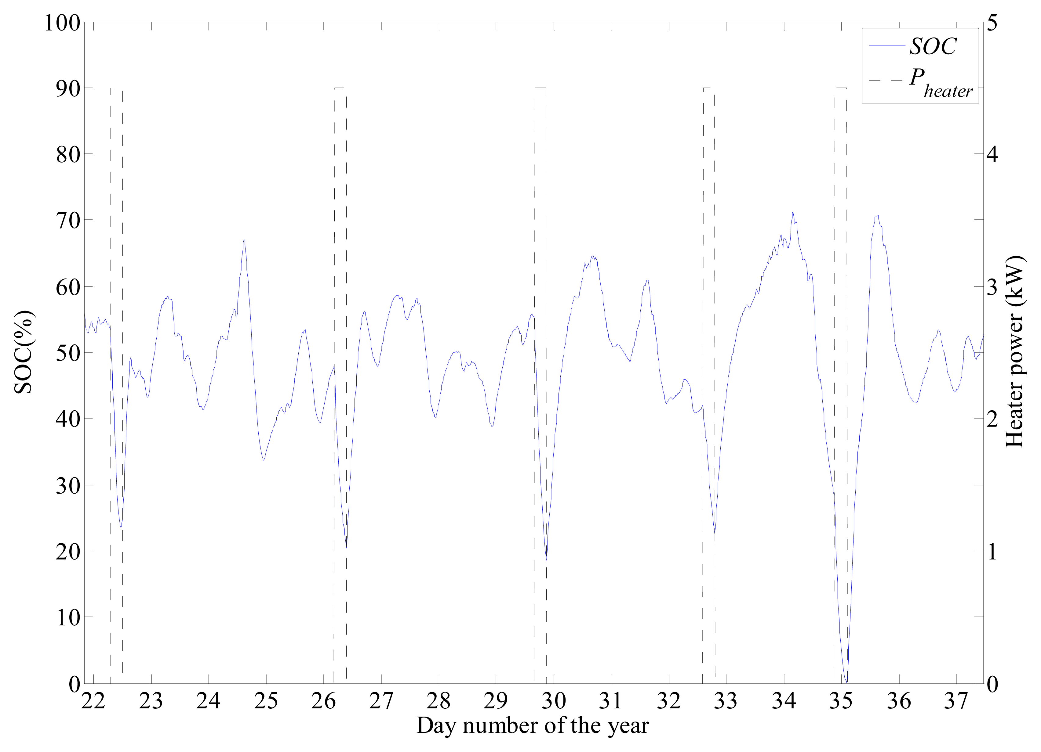
Once the microgrid is set up and the enhanced proposed strategy algorithms are all programmed in the PXI, the system is started and it remains operating and acquiring all the data continuously. Figure 22 shows different power profiles for four days of operation. The net power is shown in black, which is the power profile that the microgrid would exchange with the grid in the absence of any storage device or any strategy. Thanks to the battery, and to the appropriate energy management strategy, the power profile actually exchanged is much smoother and is represented by the blue line. The rest of the power is mainly managed by the battery, in green in Figure 22, thanks to the strategy that maintains its SOC around the desired value.
6. Conclusions
In this article, an energy management strategy for residential microgrids capable of covering all the energy demand with a very high share of renewables is proposed. The designed control improves significantly the power profile exchanged with the grid, when compared to the current state-of-the-art strategies, in terms of the reduction of both power peaks and fluctuations. In comparison with a strategy based on a simple moving average, the reduction in positive and negative power peaks is 52% and 72%, respectively, and the value of the THD is reduced by 62%.
The enhanced proposed strategy, that makes use of DSM techniques and a hybrid electro-thermal storage system, has been validated by means of simulation during a year of operation using previously measured consumption and generation data. By using the designed algorithms, the microgrid is able to adapt to the seasonal variations of both consumption and renewable generation in this kind of systems. This adaptation ability allows optimizing the use of the energy storage units, improving significantly the results obtained in relation to other strategies.
Finally, the enhanced proposed strategy has been satisfactorily validated experimentally at the microgrid sited at the Renewable Energy Laboratory at UPNa.
It should be noted that even though all the validation has been carried out for a particular scenario, the energy management strategy proposed can be applied to similar systems as its control is carried out depending on the SOC of the battery. Only some of the parameters of the EMS should be recalculated for optimal results in a different scenario.
Acknowledgments
This work was partially funded by the Government of Navarra and the FEDER funds under project “Microgrids in Navarra: design, development and implementation” and by the Spanish Ministry of Economy and Competitiveness under grant DPI2010-21671-C02-01, as well as by the European Union under the project FP7-308468, “PVCROPS-Photovoltaic Cost reduction, reliability, operational performance, prediction and simulation”.
Conflicts of Interest
The authors declare no conflict of interest.
References
- Lu, D.; Francois, B. Strategic Framework of an Energy Management of a Microgrid with a Photovoltaic-Based Active Generator. Proceedings of the 8th International Symposium on Advanced Electromechanical Motion Systems (ELECTROMOTION) & Electric Drives Joint Symposium, Lille, France, 1–3 July 2009.
- Costa, P.M.; Matos, M.A. Assessing the contribution of microgrids to the reliability of distribution networks. Electr. Power Syst. Res. 2009, 79, 382–389. [Google Scholar]
- Farias, M.F.; Battaiotto, P.E.; Cendoya, M.G. Wind Farm to Weak-Grid Connection Using UPQC Custom Power Device. Proceedings of the IEEE International Conference on Industrial Technology (ICIT), Viña del Mar, Chile, 14–17 March 2010; pp. 1745–1750.
- Yuan, X.; Wang, F.; Boroyevich, D.; Li, Y.; Burgos, R. DC-link voltage control of a full power converter for wind generator operating in weak-grid systems. Trans. Power Electron 2009, 24, 2178–2192. [Google Scholar]
- Grid Connection Code for Renewable Power Plants (RPPs) Connected to the Electricity Transmission System (TS) or the Distribution System (DS) in South Africa. Available online: http://www.nersa.org.za/Admin/Document/Editor/file/Electricity/TechnicalStandards/South%20African%20Grid%20Code%20Requirements%20for%20Renewable%20Power%20Plants%20-%20Vesion%202%206.pdf accessed on 4 October 2013.
- German EON Grid Code. High and Extra High Voltage. Available online: http://www.nerc.com/docs/pc/ivgtf/German_EON_Grid_Code.pdf accessed on 4 October 2013.
- PREPA Appendix E-PV Minimum Technical Requirements. Available online: http://www.fpsadvisorygroup.com/rso_request_for_quals/PREPA_Appendix_E_PV_Minimum_Technical_Requirements.pdf accessed on 4 October 2013.
- Budischak, C.; Sewell, D.; Thomson, H.; Mach, L.; Veron, D.E.; Kempton, W. Cost-minimized combinations of wind power, solar power and electrochemical storage, powering the grid up to 99.9% of the time. J. Power Source 2013, 225, 60–74. [Google Scholar]
- Hatziargyriou, N.; Asano, H.; Iravani, R.; Marnay, C. Microgrids: An overview of ongoing research, development, and demonstration projects. IEEE Power Energy Mag 2007, 5, 78–94. [Google Scholar]
- Tan, X.; Li, Q.; Wang, H. Advances and trends of energy storage technology in microgrid. Int. J. Electr. Power Energy Syst. 2013, 44, 179–191. [Google Scholar]
- Gkatzikis, L.; Koutsopoulos, I.; Salonidis, T. The role of aggregators in smart grid demand response markets. IEEE J. Sel. Areas Commun 2013, 31, 1247–1257. [Google Scholar]
- Masters, C.L. Voltage rise: The big issue when connecting embedded generation to long 11 kV overhead lines. Power Eng. J. 2002, 16, 5–12. [Google Scholar]
- Mahmud, M.A.; Hossain, M.J.; Pota, H.R.; Nasiruzzaman, A.B.M. Voltage Control of Distribution Networks with Distributed Generation Using Reactive Power Compensation. Proceedings of the IECON 37th Annual Conference on IEEE Industrial Electronics Society, Melbourne, Australia, 7–10 November 2011.
- Black, J.W.; Larson, R.C. Strategies to overcome network congestion in infrastructure systems. J. Ind. Syst. Eng. 2007, 1, 97–115. [Google Scholar]
- Parissis, O.-S.; Zoulias, E.; Stamatakis, E.; Sioulas, K.; Alves, L.; Martins, R.; Tsikalakis, A.; Hatziargyriou, N.; Caralis, G.; Zervos, A. Integration of wind and hydrogen technologies in the power system of Corvo island, Azores: A cost-benefit analysis. Int. J. Hydrog. Energy 2011, 36, 8143–8151. [Google Scholar]
- Shinji, T.; Sekine, T.; Akisawa, A.; Kashiwagi, T.; Fujita, G.; Matsubara, M. Reduction of power fluctuation by distributed generation in micro grid. Electr. Eng. Jpn. 2008, 163, 22–29. [Google Scholar]
- Kim, S.-K.; Jeon, J.-H.; Cho, C.-H.; Ahn, J.-B.; Kwon, S.-H. Dynamic modeling and control of a grid-connected hybrid generation system with versatile power transfer. IEEE Trans. Ind. Electron 2008, 55, 1677–1688. [Google Scholar]
- Zhou, H.; Bhattacharya, T.; Tran, D.; Siew, T.S.T.; Khambadkone, A.M. Composite energy storage system involving battery and ultracapacitor with dynamic energy management in microgrid applications. IEEE Trans. Power Electron 2011, 26, 923–930. [Google Scholar]
- Barricarte, J.J.; San Martín, I.; Sanchis, P.; Marroyo, L. Energy Management Strategies for Grid Integration of Microgrids Based on Renewable Energy Sources. Proceedings of the 10th International Conference on Sustainable Energy Technologies (SET), Istanbul, Turkey, 4–7 September 2011.
- Aviles, D.A.; Guinjoan, F.; Barricarte, J.; Marroyo, L.; Sanchis, P.; Valderrama, H. Battery Management Fuzzy Control for a Grid-Tied Microgrid with Renewable Generation. Proceedings of the IECON 38th Annual Conference on IEEE Industrial Electronics Society, Montreal, QC, Canada, 25–28 October 2012; pp. 5607–5612.
- Kriett, P.O.; Salani, M. Optimal control of a residential microgrid. Energy 2012, 42, 321–330. [Google Scholar]
- Mammoli, A.; Jones, C.B.; Barsun, H.; Dreisigmeyer, D.; Goddard, G.; Lavrova, O. Distributed Control Strategies for High-Penetration Commercial-Building-Scale Thermal Storage. Proceedings of the IEEE PES Transmission and Distribution Conference and Exposition (T&D), Orlando, FL, USA, 7–10 May 2012.
- Wang, P.; Huang, J.Y.; Ding, Y.; Loh, P.; Goel, L. Demand Side Load Management of Smart Grids Using Intelligent Trading/Metering/Billing System. Proceedings of the IEEE PES Trondheim PowerTech, Trondheim, Norway, 19–23 June 2011.
- Tsikalakis, A.G.; Hatziargyriou, N.D. Centralized control for optimizing microgrids operation. IEEE Trans. Energy Convers 2008, 23, 241–248. [Google Scholar]
- Kanchev, H.; Lu, D.; Colas, F.; Lazarov, V.; Francois, B. Energy management and operational planning of a microgrid with a PV-based active generator for smart grid applications. IEEE Trans. Ind. Electron 2011, 58, 4583–4592. [Google Scholar]
- Byeon, G.; Yoon, T.; Oh, S.; Jang, G. Energy management strategy of the dc distribution system in buildings using the EV service model. IEEE Trans. Power Electron 2013, 28, 1544–1554. [Google Scholar]
- Sauer, D.U. Electrochemical Storage for Photovoltaics. In Handbook of Photovoltaic Science and Engineering, 1st ed.; Luque, A., Hegedus, S., Eds.; Wiley: Chichester, UK, 2002; p. 847. [Google Scholar]


| Strategy used | P+ (kW) | P− (kW) | MPD (W/h) | APD (W/h) | THD |
|---|---|---|---|---|---|
| Pnet | 9.58 | −7.12 | 24,954 | 1394 | 4.34 |
| Moving average | 6.48 | −3.23 | 1819 | 228 | 2.46 |
| Preliminary | 3.10 | −0.9 | 1044 | 97 | 1.18 |
| Enhanced proposal | 2.27 | −0.9 | 707 | 39 | 0.94 |
© 2014 by the authors; licensee MDPI, Basel, Switzerland. This article is an open access article distributed under the terms and conditions of the Creative Commons Attribution license ( http://creativecommons.org/licenses/by/3.0/).
Share and Cite
Pascual, J.; Sanchis, P.; Marroyo, L. Implementation and Control of a Residential Electrothermal Microgrid Based on Renewable Energies, a Hybrid Storage System and Demand Side Management. Energies 2014, 7, 210-237. https://doi.org/10.3390/en7010210
Pascual J, Sanchis P, Marroyo L. Implementation and Control of a Residential Electrothermal Microgrid Based on Renewable Energies, a Hybrid Storage System and Demand Side Management. Energies. 2014; 7(1):210-237. https://doi.org/10.3390/en7010210
Chicago/Turabian StylePascual, Julio, Pablo Sanchis, and Luis Marroyo. 2014. "Implementation and Control of a Residential Electrothermal Microgrid Based on Renewable Energies, a Hybrid Storage System and Demand Side Management" Energies 7, no. 1: 210-237. https://doi.org/10.3390/en7010210