
Realistic Nudging through ICT Pipelines to Help Improve Energy Self-Consumption for Management in Energy Communities

1
Univ. Grenoble Alpes, CNRS, Grenoble INP, G2Elab, 38000 Grenoble, France
2
Enogrid, 38100 Grenoble, France
*
Author to whom correspondence should be addressed.
Energies 2023, 16(13), 5105; https://doi.org/10.3390/en16135105
Submission received: 16 May 2023
/
Revised: 21 June 2023
/
Accepted: 29 June 2023
/
Published: 1 July 2023
(This article belongs to the Special Issue Effective and Efficient Management Practices in Energy Sources and Energy Consumption)
Abstract
:Taking full advantage of the potentialities of renewable energies implies overcoming several specific challenges. Here, we address matching an intermittent energy supply with household demand through a nudging approach. Indeed, for households endowed with solar panels, aligning energy consumption with production may be challenging. Therefore, the aim of this study is to introduce two information and communication technology (ICT) nudging pipelines aimed at helping households integrated in energy communities with solar panels to improve their self-consumption rates, and to evaluate their efficiency on semi-real data. Our pipelines use information available in real-world settings for efficient management. They identify “green periods”, where households are encouraged to consume energy with incitation through nudging signals. We evaluate the efficiency of our pipelines on a simulation environment using semi-real data, based on well-known consumption datasets. Results show that they are efficient, compared to an optimal but unrealistic pipeline with access to complete information. They also show that there is a sweet spot for production, for which nudging is most efficient, and that a few green periods are enough to obtain significant improvements.
1. Introduction
Our work addresses challenges at the intersection of two important tropes. One is the increasing attention given to the optimisation of the energy consumption of buildings, both for economical and ecological reasons. For instance, the residential sector is known to represent about 25% of the European energy consumption [1]. One way to lower this consumption is to improve the thermal isolation of buildings. Another way is linked with the second trope, which is the increasing usage of renewable energies in energy systems [2]. Among the main renewable sources are wind, and solar, energy. While they may help lower global consumption, reduce carbon emissions, and create local generation–consumption loops, they come with specificities, with respect to traditional systems, which make taking full advantage of their potentialities a challenge. Chief among these specificities is the intermittent nature of the resulting production. This is the point we focus on in our study.
One ever more common situation, nowadays, is that of a household with photovoltaic panels on its rooftop. Consumption which is not covered by the panels is provided by the regular distribution network. It is more interesting for the household to use the solar production, rather than that brought by the energy provider. Therefore, there is much value in aligning consumption with solar production as best as possible [3]. However, alignment is not straightforward to reach.
There are two ways to improve consumption-production alignment in a building: direct and indirect flexibilities [4]. The first one refers to the automated activation or deactivation of electrical appliances through the addition of hardware and software in the consumption loop. The second refers to changes in the consumption behaviour of the users of the building. Arguably, the latter is more cost friendly and energy friendly, as it does not require the addition of equipment in the building. Moreover, it is efficient: Twum-Duah et al. [4] estimate that self-consumption could be improved by as much as in the case of a smart building, where users can reload their electrical vehicles. And Shadid [5] estimates that the intervention of nudge signal results in approximately 18% energy conservation during the orange periods when people are nudged not to consume. Additionally, during the green periods, there is an increase of over 11% in the energy self-consumption. However, while it is possible for households to try to align their consumption with solar production on their own, this often represents time-consuming work. Indeed, studies have shown that retired households more actively reduce their consumption upon receiving feedback, likely because they have more time available than working households [6]. Moreover, households may improperly assess their own consumption [7].
Therefore, there is a case for recommendation services discharging the user of most of this work and presenting them with ready-made and sharp consumption advice, like, for instance “consume on Wednesday afternoon, but not on Friday evening”. Indeed, mere feedback about consumption have already shown some efficiency in helping users reduce their energy consumption [8]. More generally, nudges [9] can be used to entice users to adopt renewable friendly consumption patterns.
The recommendations could be either provided by humans or automation. Automation, through the use of information communication technologies (ICTs) (information and communications technology refers to the use of digital technologies to manage and process information, as well as to communicate, share, and access information), is scalable, contrary to human-provided services. Indeed, it allows fast processing of the large amounts of data needed, and the concurrent generation of recommendations for all households using the service. Therefore, we use ICT nudging pipelines to construct our service. The aim of this study is to introduce two information and communication technology (ICT) nudging pipelines aimed at helping households integrated in energy communities with solar panels to improve their self-consumption rates, and to evaluate their efficiency on semi-real data. ICT pipelines designate the chain of technologies, be it hardware of software, which collect information, process it, and produce an output. In our case, they collect consumption and weather data, make algorithmic computations on those, and output advice in the form of nudges, suggesting to users when to use energy-consuming appliances.
To design the recommendations, we would ideally like to know in advance which part of their consumption the households would be willing to shift. However, this knowledge is practically impossible to obtain in real-world settings, if only because household people may not know it themselves, in advance. We therefore introduce two nudging pipelines using only information accessible in real life: aggregate past consumption of the household and weather forecasts for the future. One pipeline merely signals sunny periods, while the other predicts available production (that is, excess production with respect to the predicted consumption), thanks to load-forecasting techniques.
We show that our pipelines are efficient, even with them using real, and therefore incomplete, information, by validating them on semi-real data, coming from several publicly available datasets, coupled with a simulation environment. We intend to validate them on a real-world setting in the future but, due to the many constraints in setting-up a real-world experiment, we wanted to first test our pipeline in a simulated setting. Under reasonable user behaviour assumption, the simulator provides a first validation of our pipeline.
Our work takes place as part of ongoing efforts to help energy communities, using renewable energies, reach their full potential. This requires shifts in consumption patterns, with respect to usages linked with traditional energy sources. These changes in habit will only be possible if efforts are made to increase general consciousness about the culture changes implied and by providing accurate information to the users. We elaborate on these goals in the discussion section.
We start by presenting related works, and stating our contributions, in Section 2. Next, we introduce our model in Section 3. We then present our numerical simulation results in Section 4. Finally, we discuss our results, and their practical implications for the real-world deployment of our pipelines in Section 5. The code for the numerical simulations is available in the following repository, https://gitlab.com/enogrid/open-source/realistic-nudging-pipelines-for-energy-consumption (accessed on 30 June 2023).
2. Background Material and Contributions
We first discuss related works (Section 2.1) before making our problem statement (Section 2.2) and stating our contributions (Section 2.3).
2.1. Related Works
The energy management of buildings is a thriving area of research [10,11]. For instance, Martin Nascimento et al. [12] help assess the forecast errors of short-term forecasting models of building consumption, used in consumption planning. Reducing the error helps improve the efficiency of these tools. Pajot et al. [13] use generative modelling of building consumption to study their flexibility potential, thanks, in particular, to the OMEGAlpes optimiser [14,15]. Laicane et al. [1] assess the potential of demand-side management for consumption reduction in households. ICT technologies can be useful for energy management during unexpected, and disrupting, events [16]. More generally, the use of ICT technologies has been recognised as a crucial feature to leverage all the potentialities of smart grids endowed with renewable energies [2,17].
The notion of nudge (see in particular Thaler and Sunstein [9]) gathers any intervention aimed at making people adopt a behaviour, which they would not adopt spontaneously. Moreover, the intervention must be as light as possible so as not to become a constraint. They can take many forms (like mail or advertisement campaigns), and also differ in contents (these can be feedbacks, or “explicit injunctions”, for instance). Nudging strategies aiming at helping people improve the way they consume energy has been recognised as an interesting tool for energy consumption management: see, for instance, the review Karlin et al. [18]. Experiments have been conducted as well on private households [19,20] and on working premises [21]. Analysis of the results of the large-scale OPOWER study showed nudging to be efficient in helping reduce consumption [22]. In this study, the company sent letters to customers, contrasting their consumption with that of their neighbours. Nudging is especially interesting, as it represents a non-monetary and cost-effective way to help improve energy consumption [22]. In that regard, emails and internet platforms possess huge scalability potential. In our work, our nudges, composed of green periods (see Section 3), are similar to those defined in Salman Shadid et al. [19].
Load forecasting (Hong et al. [23] or Eliana Vivas and Salas [24]) is an important feature of many energy management tools. The methods available range from statistical methods [25] to probabilistic ones [26], or machine learning ones [27], for instance. The statistical–probabilistic family of methods includes linear models [28], autoregressive moving average (ARMA) models [29], or the ARIMA model of Box and Jenkins [30]. The methods of this family use linear processes. They are simple to implement and well adapted for the short term but unable to handle the non-linearity existing in the load series [24,31]. Machine learning approaches notably include random forests [31], K-nearest neighbors (KNN) [32], or fuzzy neural network-based forecasting methods [33]. Hybrid methods that combine artificial intelligence and metaheuristic optimisation have proved highly effective [31].
The optimisation of energy systems is a crucial question, made all the more acute by the introduction of renewable energies, while systems where not originally designed for such sources [34]. However, renewable energies introduce new constraints, like the intermittence of production, which must be taken into account in order to make for reliable systems. There exist optimisation tools aplenty [35]. However, the diversity of the models used [34] make the construction of an all-encompassing approach difficult. Hodencq et al. [15] constructed the OMEGAlpes model in such a way that it can be most easily used, and open sourced the code. Other modern approaches try to take into account as realistic assumptions as possible, which might have been overlooked at first [36]. Mathematical techniques, like mixed-integer linear programming, or genetic algorithms, are use to optimise challenging models [37].
2.2. Problem Statement
The problem we study runs as follows. On the one hand, we have a household endowed with private solar panels, which provides part of the household consumption, while the remaining part comes from the network provider. In order to better align their consumption to solar production, the people in the household are willing to shift the consumption of some of their appliances, known only to them, upon reception of a signal from an external service. The signal consists of the labelling of consumption favourable moments. However, the household people are only willing to entertain signals with a few labelled periods, as having too many of them leads to user fatigue.
On the other hand, the nudging service only has access to real, therefore incomplete, information: weather forecast, and aggregated past household consumption. Crucially, the service does not know the shiftable part of the household consumption. It strives at indicating to the household the best moments to consume.
Our problem is, therefore, how to best identify consumption favourable periods so as to help the household align their consumption to solar production, while keeping the number of labelled periods low.
2.3. Contributions
We conduct numerical simulations on a full simulator, taking into account the response of a household to nudges. The data we feed our simulator with are semi-real. We use, in particular, the well-known Iris [38] and AMPds [39] energy datasets. Our contributions are threefold.
- First, we show numerically that, even with scarce information, and even when sending nudges with a few labelled periods, we manage to achieve significant consumption improvements.
- Second, we show numerically that, in some situations which we characterise, a load-forecasting based nudging pipeline outperforms the mere “weather based” one, which targets periods with high sunshine.
- Third, we identify two important aspects concerning the efficiency of our procedure:
- (a)
- There is a sweet spot in production, at which nudging is most efficient;
- (b)
- Increasing the number of labelled periods in the nudges increases performance, but this increase levels off, and huge improvements already occur for a few periods.
Compared to previous work like Pajot et al. [14], we consider the realistic setting, where we do not know which devices are shiftable or not for the household. We validate our nudging pipeline on simulated data, which allows us to evaluate it much quicker than would be possible in a real-world experiment. Moreover, in one of our pipelines, we offer personalised advice, using an analysis of the household consumption, and production, to construct our nudge, rather than merely telling the user when the sun will shine. Though simulation is a well-established tool to assess consumption flexibilities [13], it has not yet been branched on a human behaviour model so as to experiment with a full nudging situation, at least to the best of our knowledge. For the forecasting part, we use a simple predictor detailed in the Appendix A, Appendix B and Appendix C, which offers a good trade-off between the accuracy of the predictions and the computational time required.
3. Model
We start by by presenting our household model (Section 3.1). Next, we define the self-consumption, and self-sufficiency, rates (Section 3.2). We then define the format of the nudges we use (Section 3.3) before introducing the controllers, which compute the nudges (Section 3.4). Finally, we can describe the entire nudging pipeline (Section 3.5). All main notations are gathered in Table 1.
3.1. Household
Let be the time scale at which the load is sampled, that is, a sequence of positive real numbers representing moments in time (or timestamps).
Household consumption. We consider a household which possesses several electrical appliances. Each appliance consumes energy as it is used. The consumption of an appliance is a positive sequence , together with a finite family of non-overlapping intervals , with bounds in . The are the times of the beginning of the appliance usages, and the are the ends of the usages. The load is non-zero if, and only if, there is a k (uniquely defined) such that . All residual consumption of all appliances is gathered in the “mains” appliance. The household consumption is the family of appliance consumptions. The aggregate load at time t, , is the sum over all appliances of the load at time t of each appliance, .
Shiftable appliances. An appliance may be as follows:
- Shiftable, meaning the household may be willing to shift its usage intervals, provided these periods are not too far away from the base use time, which depends on the appliance; the length of usage intervals, that is, the values , remain fixed.
- Not shiftable, meaning the times at which the appliance are used are fixed.
For instance, people in the household may be willing to shift their use of the washing machine by two to three days at most, while the time at which they use heating is fixed (when there is no demand restraint, the study of which is beyond the scope of this paper). For every shiftable appliance, there is a maximum time delay that the household people are willing to shift this appliance consumption by. The length by which appliance usages may be deferred has been estimated, for instance, by Kwon and ∅stergaard [40] or Lucas et al. [41]. Table 2 shows the time delays we assumed for every shiftable appliance. The fact that the lengths of usage intervals are fixed means, for instance, that the washing machine takes 2.5 h per usage, irrespective of when it is used.
Solar energy production. Photovoltaic panels provide the building with the energy at time t. If it is not enough to cover , the building feeds itself on the regular network to cover . If , excess production is “lost”. No storage capacity is used. At each time , a smart meter measures the aggregate load , as well as the solar production.
3.2. Self-Consumption and Self-Sufficiency Rates
We assess the energy-consumption efficiency with the two following metrics. For each , the self-consumption at time t equals : if the household consumes more () than it produces, then it self-consumes only what it has produced, that is , while if it consumes less, then it has self-consumed the amount . Let us now recall the standard definitions of the self-consumption and the self-sufficiency rates [42,43].
Definition 1
(Self-consumption rate, self-sufficiency rate). For a household consumption , and two dates , we call the self-consumption rate between and the ratio of self-consumption to the total production:
We call the self-sufficiency rate between and the ratio of self-consumption to the total consumption:
The self-consumption rate measures the ratio of the solar production which has been consumed, and the self-sufficiency rate measures the ratio of consumption which has used solar production.
3.3. Nudge
We first define the notion of nudge we use, before explicating the model of human behaviour we assume, upon the reception of a nudge. The concept of green period is inspired from Salman Shadid et al. [19].
Definition 2
(Green period, nudge). We call the green period a tuple , where are the beginning points and are the end points of the period, and is the strength of the period. A nudge is a set of green periods. We write for the set of nudges.
The number of green periods in a nudge is decided by the recommendation service. The strength of the green periods is used to rank them. The user tries to shift their consumption first to periods with high strength, as we explain below.
Model of human behaviour upon nudge reception. We use an ideal model, to evaluate the maximum ideal potential of our ICT pipelines. Upon reception of a nudge, the household people try to shift their consumption as follows. For every shiftable appliance, the following occurs:
- They check whether there are use intervals outside of the green periods;
- If so, for every green period, ranked according to their strength, they check whether shifting the use of the appliance to the green period is admissible (the new use interval is not too far away from the old use interval);
- If so, the consumption is shifted; else, nothing is done.
This behaviour upon nudge reception is ideal in the sense that the user makes full use of the information provided. Indeed, our study aims at evaluating the potential of ICT pipelines to help improve consumption. Explicitly modelling realistic behaviour upon nudge reception, and assessing its impact, represents a following step for our research.
3.4. Controllers
We define a controller as a function which computes nudges as follows, each Sunday just before midnight. Assume it is Sunday, in the evening. Let be midnight of the incoming Monday. Let be 11:30 p.m., the following Sunday. Let be the set of weather forecasts for the incoming week: this is a set with weather forecast data for the sunshine coefficient, the temperature, and other likewise data, which the controller might use to compute the nudge. Let be the set of past household data available upon nudge computation: these are the past aggregate load and the past production.
Definition 3
(Controller). A controller is a function taking as arguments weather forecasts and past household aggregate consumption data, and outputting a nudge, that is, a function
On Monday, the household receives the nudge, and the user adapts or not their consumption for the week.
Designing good controllers is not straightforward. Indeed, write as the household consumption once modified from according to the nudge. Then, find the best possible nudge amounts for solving either of the optimisation problems (which are equivalent when production is fixed):
which means maximising either the self-consumption rate or the self-sufficiency rate of the household, over the coming week, for the nudged consumption . What complicates matters is that the effect that the nudge has on the consumption is unknown to the controller. Therefore, they have to make guesses as to what would lend itself to efficient nudges. Conversely, the household people know the effect that a nudge has on them; however, the optimisation problem they would have to solve would be too burdensome for us to expect most households to solve it every week. Therefore, to compute nudges, we do not solve these optimisation problems, but introduce the following two heuristic controllers. We validate their efficiency in our numerical simulations.
Weather controller: The first one is called “weather controller”. It takes as input the sunshine coefficient forecast for the coming week. It averages the predicted sunshine coefficient over 2 h periods. The strength parameter is set to these values. Namely, if is the forecast of the sunshine coefficient at time , then the strength parameter at time equals
(There are four half-hours in two hours, and we use a time scale of 30 min steps.) Then, it ranks the periods according to their strength, and outputs the three (say) best periods. The weather controller therefore signals the periods when it is most sunny, as they are those with the most solar production.
Combined controller: The second controller is called “combined controller”. It takes as inputs the sunshine coefficient forecast for the coming week, together with past aggregate consumption data, and past production data. It then uses load forecasting techniques to forecast excess production, that is, the difference between forecast production and forecast consumption (see Appendix C for details). It averages the predicted excess over 2 h periods, and sets the strength parameter to these averages. Finally, it outputs the three (say) best periods. Precisely, writing the forecast load at time t, and the forecast production at the same time, the predicted excess is
Then, the strength parameter at time equals
The combined controller therefore signals periods when there will be (if the forecast is accurate) the most excess. The idea is that there may be sunny periods where consumption will be high. In these periods, spare solar production will be low. As a result, shifting more consumption to these periods will not help. Therefore, by forecasting excess production, the combined controller manages to identify periods, shifting consumption to which is profitable.
3.5. Nudging Pipeline
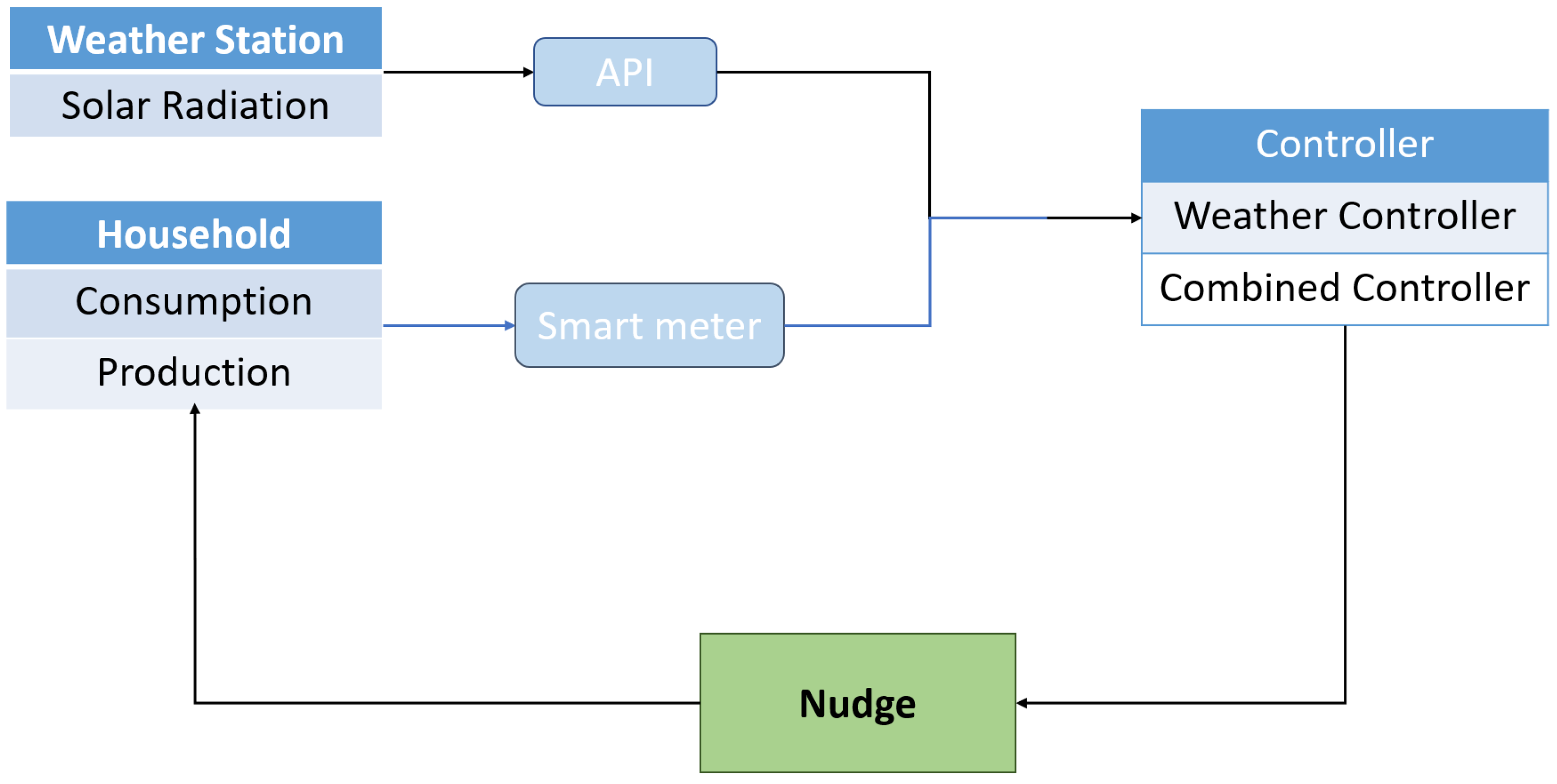
Therefore, the system “household + controller” is a controlled system, illustrated on Figure 1. The nudging pipeline, which represents the system, save for the human behaviour part, consists of the following several components. Production and consumption data are monitored by a smart sensor located on the household premises. Weather APIs provide us with accurate forecasts for the upcoming days, in particular, concerning solar irradiance. All information is gathered by the controllers, which use it to compute solar consumption-friendly periods. These periods are gathered into nudges, which are sent to the household people through emails, for instance. Finally, upon receiving the nudge, the household people update their consumption accordingly.
4. Numerical Simulations
We first describe our numerical simulations set-up (Section 4.1). Then, we show the results of simulations on synthetic data (Section 4.2 and Section 4.3) and the results of simulations on semi-real data (Section 4.4 and Section 4.5). Finally, we study the influence of the capacity of production installed (Section 4.6) and of the number of green periods in the nudges (Section 4.7) on the nudging pipeline efficiency.
4.1. Numerical Simulations Set-Up
Synthetic data preparation. We generated two synthetic datasets, representing two use cases: a commuting household (a commuting household refers to a group of individuals who live together in the same residence but travel to different locations for work or school, typically on a regular basis), and a non-commuting household (a non-commuting household refers to a group of individuals who live and work in the same place, without the need for regular travel to a workplace or school). The commuting household represents, for instance, the household of people going to work away from home but who have equipped their domestic electrical appliances with sensors, allowing them to launch, or stop, these appliances, remotely. The non-commuting household represents, for instance, the household of people working remotely.
For each household, we use as fixed consumption (that is, not shiftable), the not-shiftable part of the consumption of a real energy profile (which is part of the Iris dataset [38]). To create shiftable consumption, we add real dishwasher consumption to the data every day in the morning, real washing machine consumption every three days in the evening, and a real water heater for domestic hot water consumption every day in the evening. Therefore, the shiftable part of the consumption occurs in the morning or in the evening, and is thus representative of that of a commuting household.
For the “non-commuting household”, we add an additional electric cooker every day between 12 p.m. and 1:30 p.m., and an additional air conditioner between 12 p.m. and 4 p.m. As the people of the household are present during the day, they must cook their lunch, and they may use air conditioning to maintain agreeable temperatures within the house in the afternoon. This may be the case, for instance, for a French household, endowed with air conditioning. While it is common in France to cook at lunch, air conditioning is not as widespread as in the United States of America, for instance, but its usage is nonetheless increasing. We classify air conditioning as non-shiftable in this context of someone working from home during the afternoon in a potentially badly isolated building. In such conditions, in order to maintain cool temperatures, the air conditioning system may need to run continuously.
Real datasets preparation. For the simulations using real datasets, we select a subset of appliances, which we define to be “shiftable”, and we fix their maximum shifting delay (see Table 2 for details). We divide each dataset into past data, on which we train our model, and future data, on which we conduct the simulation. Finally, we renormalise the data sampling steps to 30 min steps.
The AMPds (Almanac of Minutely Power dataset) [39] is a publicly available dataset created by Simon Fraser University’s (SFU) Electricity and Power Research Centre in Canada. It offers high-resolution energy consumption data collected from residential households. The dataset covers the period from 2012 to 2014 and includes measurements of electricity, water, and natural gas usage at one-minute intervals for an individual building in Canada. It can be found on the project’s official website http://ampds.org/ (accessed on 30 June 2023) or through various data repositories and academic platforms.
The Iris dataset is a subset of a European database of residential consumption collected as part of the REMODECE (Residential Monitoring to Decrease Energy Consumption) project [38]. The REMODECE project is an initiative focused on monitoring and reducing energy consumption in residential buildings. It aims to develop innovative solutions and technologies to promote energy efficiency and sustainability in the residential sector. The Iris dataset contains the energy consumption data of 98 houses for a span of one year. The data sampling step is 10 min. We make the appliance names homogeneous between the houses, as there are sometimes small variations in the terminology.
Solar energy production. As part of our simulator, we generate an artificial solar production as follows. We first simulate a sunshine coefficient as the product between the following:
- A value taking into account the time of day (representing the fact there is no sun at night);
- A value taking into account the month of year (representing the fact that the sun shines brighter during summer than winter);
- A value taking into account the amount of clouds (representing the fact that more clouds implies less light for photovoltaic panels).
The process giving the amounts of clouds is simulated by Markov Chain transitioning between five levels of clouds, from “sunny” to “awful weather”. The chain is designed so that periods of sunshine alternate with cloudy periods. Precisely, write P as the stochastic matrix such that each coordinate is the probability of the chain going to state j, given that it is currently in i. Therefore, each line is a probability distribution. The chain is a discrete time chain, and for each , represents the weather between the times hours and hours. As a result, to simulate trajectories of the chain, we start at , and for , we simulate according to
Finally, the solar production generated by the panels from this synthetic sunshine coefficient is simulated as a linear function of the sunshine coefficient, that was renormalised before to the segment . The maximum power possible, that is, the capacity of the solar panels, is 3000 W.
Controllers. We use three controllers and an upper-bounding optimiser:
- The weather controller and combined controller, defined in Section 3.4, whose performance we want to assess.
- The “no control” controller, and the “OMEGAlpes” optimiser, described below, which we use as references.
The “no control” controller represents the worst case, when there are no nudges. We call it “reference” in the plots. OMEGAlpes [15] provides an upper-bound for the best possible case. It is a linear optimisation energy system modelling tool (see Appendix A for details). It computes the best possible shifting of the consumption. However, it uses data, like detailed knowledge of the shiftable consumption of the household, and therefore cannot be used in real life. Moreover, OMEGAlpes has no restrictions on the number of the formal equivalent of green periods it uses. Therefore, OMEGAlpes is not a controller in the sense of Definition 3 but provides an upper bound on the possible performance of the controllers. We provide some context about the way OMEGAlpes computes its solution in Appendix A. The nudges sent by our controllers each contain four green periods.
Simulation. The simulations run over one month. For each setting, we run 20 simulations to account for the stochasticity of the production generation.
Metrics displayed. We display the self-consumption rates of the household, for the different controllers and OMEGAlpes. We also display the improvement of our controllers (self-consumption rate with the controller minus the self-consumption rate with no controller), as a percentage of the improvement of OMEGAlpes (self-consumption rate with OMEGAlpes minus self-consumption rate with no controller). For each statistic, we show its mean, as well as the 10–90% interval of values. The results for the self-production rates are similar to those with the self-consumption rate. We present them in Appendix B.
4.2. Synthetic Data, Commuting Household
We first present the results for the synthetic commuting household. We show in Table 3 the self-consumption rate of the household, under the different controllers, and OMEGAlpes. We see both the weather and combined controllers improve the self-consumption rate, with respect to the “no control” reference. In average, with “no control”, the rate is 67.4%, while it is 77.35% for the weather controller and 77.63% for the combined controller. We also show the performance of our controllers as percentages of that of OMEGAlpes. They range between 45.9% and 47.25%. Clearly, we cannot obtain the full improvements of OMEGAlpes with our nudges, but we can still obtain a significant part of it.
4.3. Synthetic Data, Non-Commuting Household
In the non-commuting scenario, a large, not-shiftable consumption (due to the electric cooker and the air conditioner) takes place in the afternoons, when solar production is potentially at its maximum. Therefore, even if there is a lot of production in the afternoons, there is not a lot of excess production. As a consequence, looking at the sunshine coefficient to identify green periods will be misleading, as we now see. In Table 4, we see that the self-consumption rate with the intervention of the Combined Controller (93.82% on average) is significantly higher than that with the Weather Controller (90.9% on average). Indeed, the percentage of improvement, with respect to the OMEGAlpes reference, of the Combined Controller, is more than 29% that of the Weather Controller (average of 47.94% against 18.53%). This happens because the Weather Controller only considers periods when the weather is favourable for production, but does not take into account the household’s consumption patterns. As a result, it may identify a green period when there is a high production, without noticing there is also a high consumption taking place. It may therefore encourage people to shift consumption to a moment where production is already saturated. On the other hand, by forecasting consumption as well as production, the Combined Controller is able to identify moments where there is likely to be excess production. Shifting consumption to these moments therefore helps improve the self-consumption rate.
4.4. Iris Dataset and AMPds Dataset, Individual Building Simulation
We first run a simulation for an individual building of Iris and the AMPds building. We show on Table 5 the results of the simulation for Iris and AMPds. We see that both the weather and the combined controllers manage to improve the self-consumption rate of the building, taking it from 63.13% to more than 66.77% (weather) and 67.9% (combined). Results are comparable for AMPds: we see that both the controllers improve the self-consumption rates from 70.86% to more than 70.92%. The fact that the performance results of the two controllers are close is probably due to the fact that excess production occurs mainly when the absolute production is high (contrary to the use case of Section 4.3). We note that even the worse results of the controllers are better than all but the very best results of the reference situation, in which there is no control, which shows the value of our procedure.
4.5. Iris Dataset, Collective Runs
Then, we conduct simulations for all the buildings of the Iris dataset, and show the results on Table 6. The mean, and mean of the percentage of improvement, are averaged on all the buildings. We see that, on average, the weather and combined controllers improve the self-consumption rate by about 2%. This corresponds to roughly 17–22% of the OMEGAlpes performance. While the results of OMEGAlpes are much higher than that of the controllers, we believe it is mainly due to the limitless number of shifts in consumption it can perform and the fact that it uses per-appliance knowledge of the true consumption. Therefore, given these advantages, we believe reaching 22% of its performance, in the case of the combined controller, still shows the reasonable efficiency of our nudging pipelines.
To look at the influence of energy flexibility on the enhancements in the self-consumption rate, we conducted simulations on three distinct subsets of the Iris dataset, based on the numbers of shiftable appliances in each house: 1, 2, or 3. We show on Table 7 the results of the simulations. Unsurprisingly, the greater the number of shiftable appliances within the houses, the greater the self-consumption rate increases when nudges are sent (going from 1% for the first dataset, to 4% for the third one), under similar conditions, such as weather and house type.
4.6. Influence of the Amount of Production
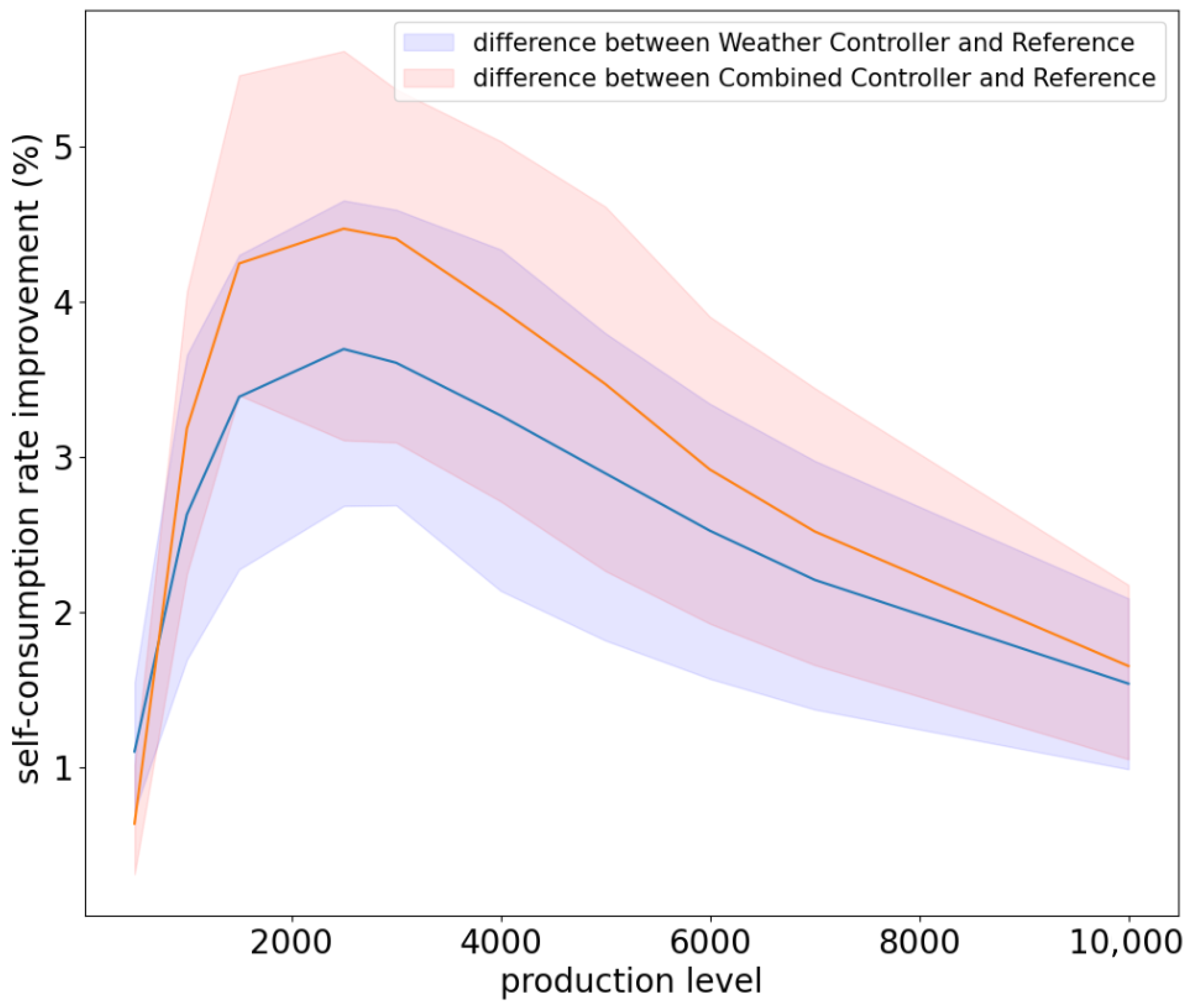
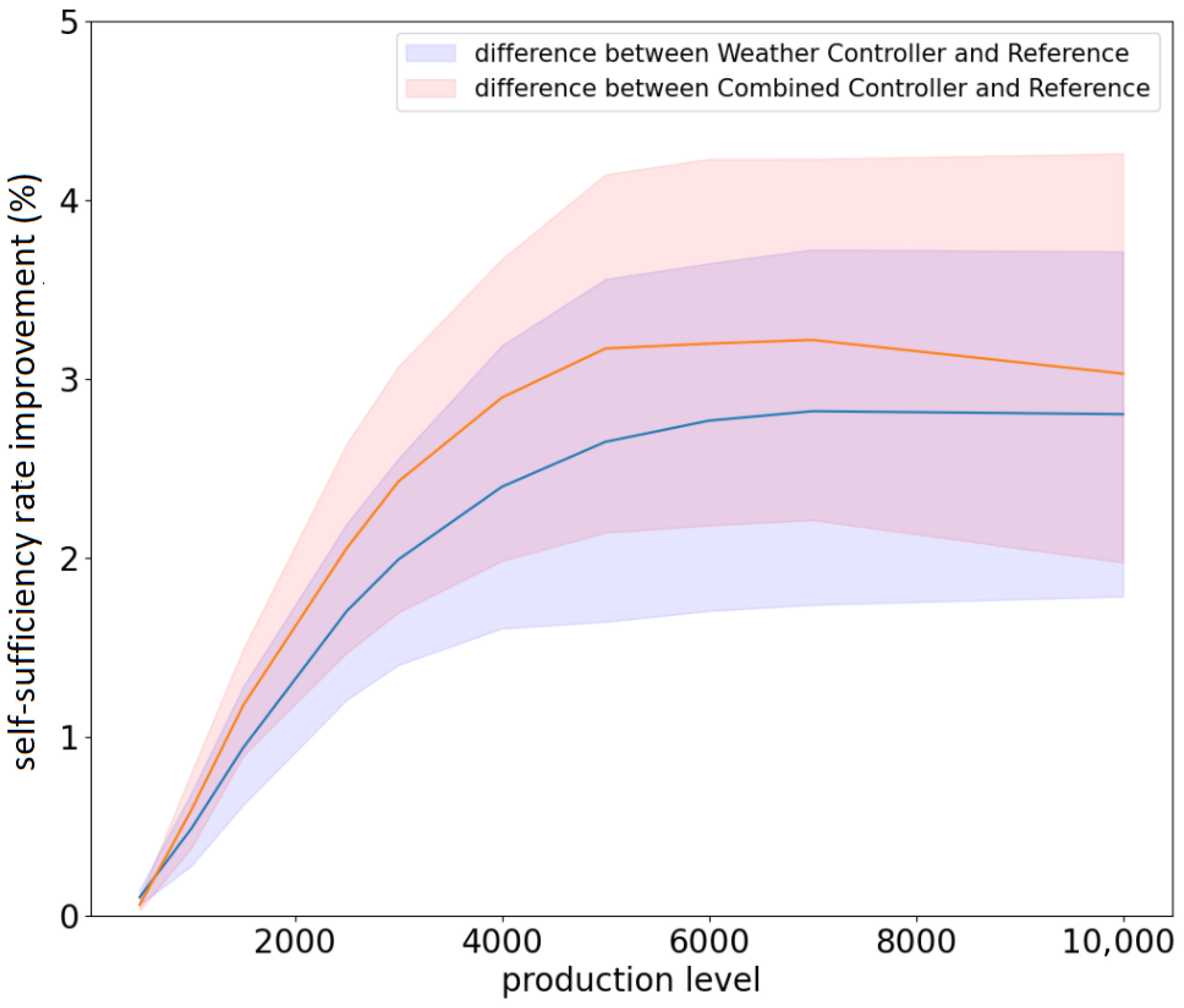
We show on Figure 2 the increase in the self-consumption rate, for the Iris household, as a function of the amount of maximum possible production (this amount increases when more solar panels are installed). We see that the increase in the self-consumption rate is maximal for a production between 2000 and 3000 W for both cases of controllers and that it decreases for lower, and larger, values of production. Indeed, when there is very little production, there are not many gains to target by shifting consumption; therefore, nudging does not help a lot. Likewise, when there is a lot of production, all consumption already takes place when solar production is high, and therefore, there is no need to shift consumption. On the contrary, for intermediate values of production, shifting may help improve self-consumption, and therefore nudging proves valuable. Finally, we see that the superiority of the combined controller over the weather controller is highest in the production range where nudges are most efficient. This strengthens the case for using the combined controller.
4.7. Influence of the Number of Green Periods
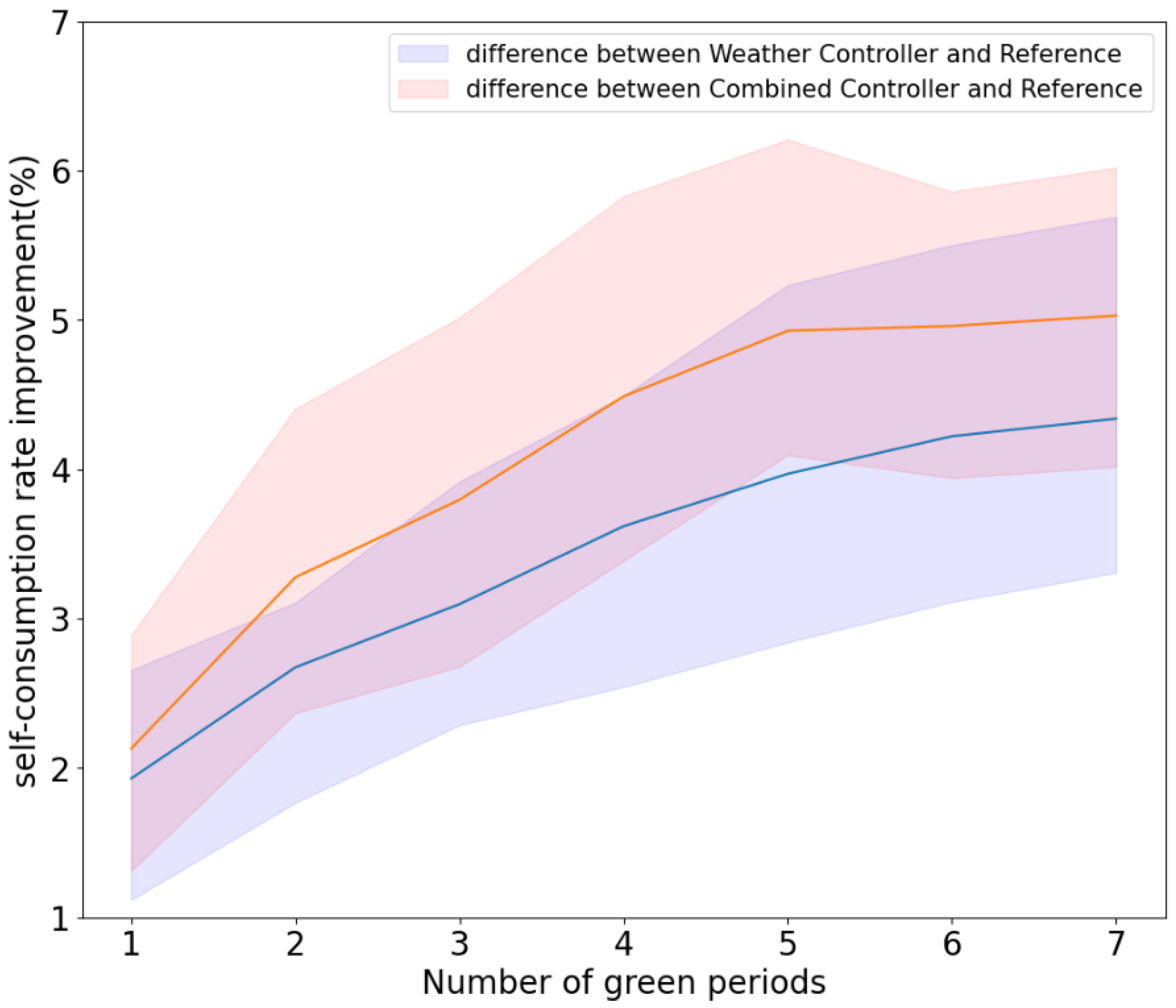
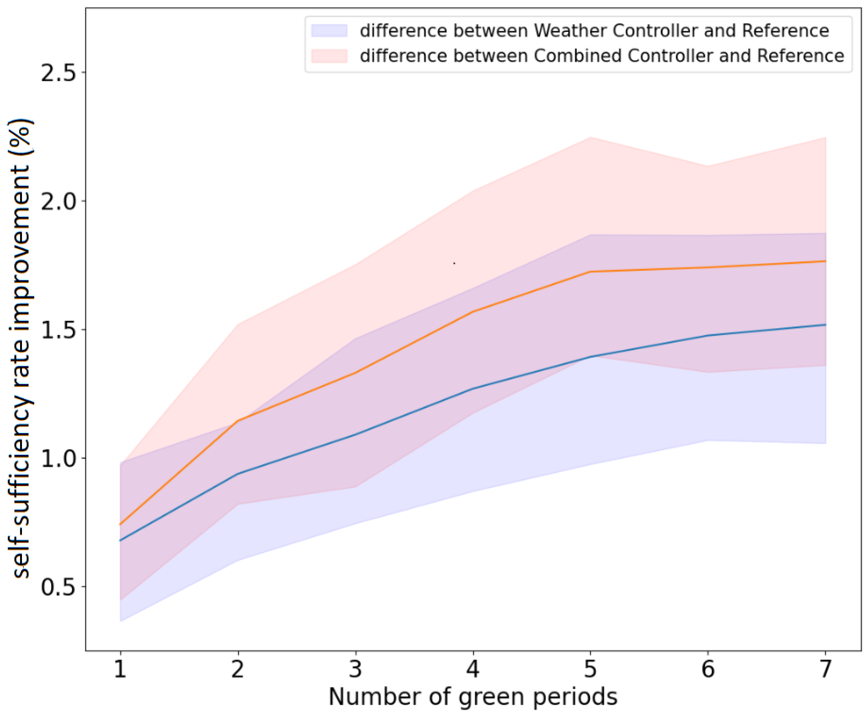
We show on Figure 3 the efficiency of nudges as a function of the number of green periods in each nudge. This matters, as, realistically, users will tire if presented with too much information. Therefore, we should strive to send nudges with as few green periods as possible. However, we must make sure the efficiency of the nudge remains satisfying. The augmentation of the self-consumption rate increases with the number of green periods of a week, which is expected. However, the slope of the curve decreases as the number of green periods increases. This means that every supplementary green period helps to increase the self-consumption rate less than the previous. As a result, we see that most gains are concentrated on the left of the plot, from 0 to 4 green periods by nudge, and that gains realised by adding more green periods are lower and lower. This is probably due to the fact that the most easily shiftable consumption is already shifted with fewer nudges. We therefore recommend that each weekly nudge contains three or four green periods, as it strikes a good compromise between having an efficient procedure and avoiding user fatigue.
5. Discussion and Conclusions
We showed on semi-real data, in a simulated environment, that our ICT nudging pipelines using real-world accessible information were efficient in helping households improve their self-consumption. We showed that forecasting excess production, and constructing nudges based on this, beats merely providing weather forecasts when maximum solar production and excess production do not take place at the same time. We observed that the more flexibility there is in a household, the more profitable sending nudges is. Moreover, we saw that there is a sweet spot in production, for which nudging is most efficient. Indeed, when production is too small, or too large, there are few improvements to obtain by shifting consumption. Finally, we saw that most gains in self-consumption take place with few “green periods” by nudge, which is encouraging, as limiting their number helps prevent user fatigue.
While our results show that we can obtain reasonable performance with respect to the OMEGAlpes reference, we also saw that absolute improvements in the self-consumption and self-sufficiency rates, by merely shifting some part of the consumption upon nudge reception, are not enough to reach close to one rates. This probably entails that selectively reducing usage may be somewhat necessary for households willing to reach much better rates. Note that this may not necessarily mean a reduction in the “comfort” provided by appliances usage, as “unnecessary” usages, like appliances left in sleep mode instead of being turned off, may be removed, without diminishing the benefits one obtains from the appliance.
One takeaway of our study is the importance of assessing both the hardware and the “human”, so to speak, components of the household to identify settings where nudging will be efficient. Indeed, on the one hand, the photovoltaic capacity must be in the “sweet spot” we identified. On the other hand, the household people must be willing to shift enough of their consumption for these shifts to truly weigh on the part of solar energy used, with respect to the standard energy. In turn, making these assessments requires patient ground work, collecting individual information about photovoltaic capacity and consumption usages. This may seem like time-consuming effort, while nudge pipelines are supposed to be easy to set-up, but they can be viewed as a “one-off”, initial investment before letting the nudging pipeline run automatically.
We intend to pursue our work by testing our nudge scheme in real-world situations. Thanks to our simulations, we can have some confidence that it will be efficient, without overburdening users with information. Indeed, one important take of our simulations is the fact we can restrict our weekly nudges to three or four green periods, while still achieving satisfying results. It seems reasonable to imagine users mentally flagging these three to four periods during the week, and attempt to shift some consumption to these. Of course, we will have to test this assumption, first by directly asking the users, and second, by monitoring the key consumption metrics to quantify the effect our pipelines have on user consumption. As far as the controller choice is concerned, we will deploy the weather adviser for households where solar production and excess production tend to be correlated, and the combined controller for the others. Of course, we might also attempt to shift controllers as time goes on. Finally, before deploying a nudging scheme, we will assess whether the solar panel capacity is indeed in the range where nudging might be profitable, as our simulations showed that there would be no interest in doing so, should it be insufficient, or too large.
However, two main limitations of our work will need to be addressed for our pipelines to prove efficient in real-world settings. The first limitation stems from the complexity of human behaviour in real-life situations, as individuals vary in their reception and response to information. In our simulations, we assumed idealised human behaviour, whereby the household people would try their utmost to comply with the suggestions in the nudge. This may not be the case in real life, not for all individuals, in any case. Thus, future research directions should focus on estimating the “compliance” rate of users receiving nudge, and devising ways to make this rate improve. The second limitation pertains to the energy and weather forecasting modules. We used a simple energy forecasting module, which will probably require enhancing to remain relevant in real-world situations. Fortunately, there are many possible models available in the literature, which we may use. However, even state-of-the-art weather forecasts may prove inaccurate, especially a few days down the line. The prediction errors, about energy usage, and weather, can potentially result in incorrect information about green periods. This may lead to bad consumption shifts from the users, and potentially discourage them from further using the scheme. One way to make the forecast more robust would be to use ensemble models, which gather forecast from several models, and construct an aggregated forecast from these, which often proves more reliable than any one taken separately.
We have so far based our recommendations on the aggregate knowledge of the building consumption. Now, we could formulate better nudges if we had finer knowledge of the building consumption (the energy flexibility in the building). Non-intrusive load monitoring is the field concerned with gaining knowledge about the inner consumption of a building, without having to equip all its devices with ad hoc sensors [44]. In spite of its inherent difficulty, as a blind source separation problem, valuable results have been obtained through numerous procedures (see, for instance, Zhong et al. [45], which uses hidden Markov models, or Zhang et al. [46] which uses neural networks, for machine learning approaches). Branching one such procedure in our nudging pipeline would likely improve it.
In our work, we considered the case of an individual building. Now, thanks to recent legislation (see Commission de Régulation de l’énergie [47] for the case of France, Di Silvestre et al. [48] for that of Italy, and Solar Power Europe [49] for a broader view of the European Union), it is possible for building owners to create an association and share their production with the members: this is called collective self-consumption. Now, the alignment of consumption with production is made more complex by the fact that there are several consumers. Designing efficient nudging strategies also becomes more complex. For instance, telling everyone that there will be a sunny afternoon may result in excess consumption, due to all members shifting their production at the same time. We intend to further our work in this interesting and challenging direction in order to try to contribute to realising the potential that these communities have to get close to zero net energy consumption. This means that all energy used within the community is also produced within the community (the equivalent, in the case of the community, to “zero consumption on the meter” for an individual household) and is one of the very important potential benefits of these communities.
We believe there are two main difficulties in deploying solar energy, related to user adoption. The first is the cultural shift required to fully exploit it. Indeed, people are not used to looking at the weather before using their washing machine, for instance. Adapting behaviours accordingly will require time. This will only be possible through the adoption of this energy. However, this runs into the second difficulty: user experience is, at least in the beginning, downgraded when one gives up using “standard” energy sources and starts to use solar energy. Indeed, consuming whenever one sees fit is more convenient than taking into account the new constraint that one must pay attention to the sun. Of course, there are advantages to doing this, of economical and environmental kinds, but these are not immediately apparent, contrary to the inconvenience of having to take into account the sun. The widespread adoption of solar energy will therefore require efforts in order to make the transition as seamless as possible. We believe that deploying recommendation services, providing just enough information to help users take advantage of the solar energy, in as non-intrusive of a way as possible, will play a huge part in reaching this aim.
Author Contributions
H.L. is the main author and this work was realized as part of his Ph.D.; P.-Y.M. contributed as a secondary author and senior advisor; T.R. and F.W. contributed to the overall reflection on the study. All authors have read and agreed to the published version of the manuscript.
Funding
This work was partially supported by the ANR project ANR-15-IDEX-02 through the eco-SESA project, https://ecosesa.univ-grenoble-alpes.fr (accessed on 30 June 2023) and the OTE—Observatory of Transition for Energy, https://ote.univ-grenoble-alpes.fr (accessed on 30 June 2023).
Data Availability Statement
The ADMPS dataset is publicly available online at the url http://ampds.org (accessed on 30 June 2023). The Iris dataset is proprietary, so it can not be made public due to privacy reasons.
Conflicts of Interest
Haicheng Ling and Pierre-Yves Massé are employees of Enogrid. Thibault Rihet is a founder of Enogrid.
Appendix A. OMEGAlpes
We use OMEGAlpes, defined in Hodencq et al. [15], to provide an upper bound for the performance of our controllers. To give the reader an idea of how OMEGAlpes computes this bound, we provide some elements of context here. We first describe quickly OMEGAlpes (Appendix A.1), then we detail the optimisation model (Appendix A.2).
Appendix A.1. OMEGAlpes Presentation
OMEGAlpes (Optimization Models Generation As Linear Programs for Energy System) is a simulation platform developed by the Grenoble Electrical Engineering Laboratory (G2ELab) at the Grenoble Institute of Engineering and Management. It models and simulates electrical power systems, particularly those using renewable energy sources. It allows users to optimise power generation, distribution, and consumption, while respecting operational constraints. The optimisation module uses mixed integer linear programming (mixed integer linear programming (MILP) is a set of mathematical optimisation techniques used to solve problems that involve both continuous and integer decision variables in the objective function and constraints).
OMEGAlpes uses a modular architecture that allows users to build and customise simulation models according to their specific needs. The platform includes a wide range of simulation tools, such as power flow analysis and optimisation algorithms, which can be used to evaluate the performance of power systems under different scenarios and conditions.
OMEGAlpes has been used in numerous research projects and industrial applications, and it is actively developed and maintained by the G2ELab team.
Appendix A.2. Self-Consumption System Modelling
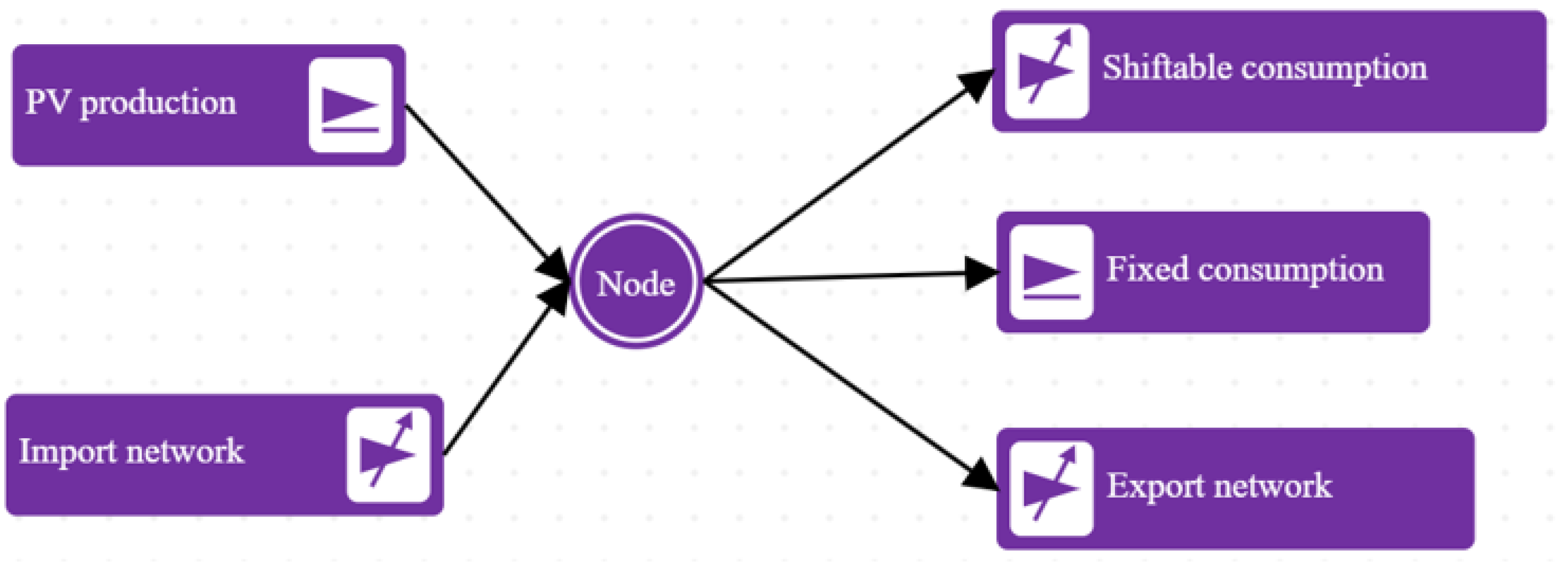
Figure A1 presents a diagram of the OMEGAlpes model implemented in the self-consumption system. The system is composed of two fixed energy units: the solar energy production unit, and the non-shiftable part of the total energy consumption. Additionally, the system includes three variable energy units: the energy imported from the grid, the energy exported to the grid, and the aggregated shiftable part of the total energy consumption. The shiftable energy part is subject to change, affecting the imported and exported energy from the grid accordingly. All energy units are interconnected to an electric node, in which the energy equations are formulated, as shown below. The equation variables are defined in Table A1.
Figure A1.
OMEGAlpes model for a self-consumption system.


Table A1.
Energy equations variables and their meaning.
| Symbol | Description |
|---|---|
| t | The time period of optimisation, denoted by , is defined as starting from , the beginning of optimisation, and ending at , the completion of optimisation. |
| The change in time depends on the frequency/sample rate of the energy profile. | |
| Power imported from the electric grid. | |
| Power exported to the grid. | |
| Network import status. It is a binary variable, a value of 1 indicates that the import from the grid is active, while a value of 0 indicates that the import from the grid is inactive. | |
| Network export status. It is a binary variable, a value of 1 indicates that the export to the grid is active, while a value of 0 indicates that the export to the grid is inactive. | |
| Power generated by the solar energy unit. | |
| Power of the shiftable part of the total consumption. | |
| Shiftable consumption status. It is a binary variable, a value of 1 indicates that the shiftable consumption is active, while a value of 0 indicates that there is no shiftable consumption. | |
| The shiftable consumption start-up is represented by a binary variable. It equals 1 only when the shiftable consumption starts, i.e., when changes from 0 to 1. | |
| Power of the non shiftable part of the total consumption. | |
| Total shiftable consumption. | |
| List of power profiles to shift. |
- Energy balance equation.
The energy balance equation in electrical systems states that the net energy flux across any node must be zero, i.e., the sum of the energy entering the node must be equal to the sum of the energy leaving the node.
- Constraint equations.
The simultaneous import and export of energy from the grid is prevented through the use of binary values, and , which indicate the activation status of importing and exporting energy, respectively. So, the sum of and is always equal to 1:
The total energy of a system should remain constant regardless of where the shiftable consumption is allocated within the system:
The following equation represents the constraint for detecting the start-up of shiftable consumption. It is defined as a binary value, which equals 1 only when the shiftable consumption starts:
The following equation ensures that the sequence of shiftable consumption is respected during optimisation. For instance, if a washing machine functions from 8 p.m. to 9:30 p.m., the “block” it represents will be shifted as a block. It will not be decomposed into several sub-blocks (of 1 h, or 30 min, for instance):
- Objective equation.
The objective of the optimisation model is to maximise the self-consumption rate in the self-consumption system, which is equivalent to minimising the energy exported to the grid.
The shiftable part of the energy consumption can be rescheduled by solving the above equations using OMEGAlpes, with the aim of maximising self-consumption in the self-consumption system. Before optimisation, a TimeUnit of OMEGAlpes must be set to define the time intervals for rescheduling. In our study, we selected a window of three days as the time constraint for rescheduling. This means that all shiftable consumption can only be rescheduled within these time periods. When optimising over a one-month period, the model maximises the self-consumption rate for each continuous three-day interval.
Appendix B. Self-Production Rates Results
We present here the results concerning the self-productions rates of all our simulations on synthetic data and on semi-real data. They are similar to those about the self-consumption rate, and we only discuss them briefly.
- Synthetic data, efficiency of nudges. We see on Table A2 that weather and combined controllers improve the self-production rate, in the case of synthetic data.
- Synthetic data, production not correlated with excess. When production is no longer correlated with excess production, the combined controller outperforms the weather controller: we see it in Table A3.
- Iris dataset and AMPds dataset, individual building simulation. Table A4 shows the performance results in the case of the Iris individual building and the AMPds building.
- Iris dataset, collective runs. We see in Table A5 the results averaged over all the buildings of the Iris dataset. The performance results are the same as for the self-consumption rate.
- Influence of the amount of production. Figure A2 shows that as the production level increases, the improvement in the self-production rate also increases; however, at a certain point (7000–8000 W), the increase in the self-production rate reaches a plateau and stops growing. All daylight consumption is already covered by solar production, so there is no longer room for improvement.
- Influence of the Number of Green Periods. Finally, we can see on Figure A3 that the efficiency of the nudges is already quite good for four periods.
Table A2.
Mean self-production rate and mean improvement ratio with various controllers, synthetic data and general case.
Table A2.
Mean self-production rate and mean improvement ratio with various controllers, synthetic data and general case.
| Reference | Weather Controller | Combined Controller | OMEGAlpes | |
|---|---|---|---|---|
| Mean (%) | 25.17 | 28.91 | 29.01 | 33.35 |
| Mean of improvement ratio (%) | 0 | 45.9 | 47.25 | 100 |
Table A3.
Mean self-production rate and mean improvement ratio with various controllers, synthetic data, uncorrelated production and excess production.
Table A3.
Mean self-production rate and mean improvement ratio with various controllers, synthetic data, uncorrelated production and excess production.
| Reference | Weather Controller | Combined Controller | OMEGAlpes | |
|---|---|---|---|---|
| Mean (%) | 22.36 | 22.79 | 23.53 | 24.85 |
| Mean of improvement ratio (%) | 0 | 18.53 | 47.94 | 100 |
Table A4.
Mean self-production rate, and mean improvement ratio, with various controllers, Iris 966 and AMPds.
Table A4.
Mean self-production rate, and mean improvement ratio, with various controllers, Iris 966 and AMPds.
| Reference | Weather Controller | Combined Controller | OMEGAlpes | |
|---|---|---|---|---|
| Iris: Mean(%) | 22.53 | 23.83 | 24.25 | 28.63 |
| AMPds: Mean (%) | 34.44 | 34.84 | 34.86 | 35.84 |
| Iris: Mean of improvement ratio (%) | 0 | 21.37 | 27.99 | 100 |
| AMPds: Mean of improvement ratio (%) | 0 | 27.74 | 29.72 | 100 |
Table A5.
Mean of self-production rate and mean of the improvement ratio with various controllers, collective simulation on the Iris dataset.
Table A5.
Mean of self-production rate and mean of the improvement ratio with various controllers, collective simulation on the Iris dataset.
| Reference | Weather Controller | Combined Controller | OMEGAlpes | |
|---|---|---|---|---|
| Mean (%) | 28.07 | 28.75 | 28.93 | 32.16 |
| Mean of improvement ratio (%) | 0 | 17.22 | 21.6 | 100 |
Figure A2.
Augmentation of the self-production rate due to the combined controller (orange)/weather controller (blue) with respect to a reference with no controller as a function of the production.
Figure A2.
Augmentation of the self-production rate due to the combined controller (orange)/weather controller (blue) with respect to a reference with no controller as a function of the production.

Figure A3.
Augmentation of the self-production rate due to the combined controller (orange)/weather controller (blue) with respect to a reference with no controller, as a function of the number of green periods by nudge.
Figure A3.
Augmentation of the self-production rate due to the combined controller (orange)/weather controller (blue) with respect to a reference with no controller, as a function of the number of green periods by nudge.

Appendix C. Load Forecasting
We use a very simple forecasting model, as it allows us to quickly test our pipelines, while leaving open the possibility to improve it or replace it with more involved models if the need arises. Indeed, our goal in building the predictor was to assess, in principle, the relevance of the combined controller (Section 3.4), which is a controller producing nudges based on forecast excess production. Upon deployment in production, we will probably use more involved forecast models.
As a forecaster for production, we use a linear model, whereby
where p is the predicted solar production, the sunshine coefficient is a value in quantifying how much sun irradiance there is, and is the regression parameter. We estimate it on past data. Now, in our simulator, solar production is by design a linear function of the sunshine coefficient (see Section 4.1). Of course, in real life, this will no longer be the case, and a linear model will probably show bad performance results for the production forecast. We will use more involved models in that case.
As a forecaster for consumption, we create a week consumption profile by averaging the past data over a week. Then, the consumption of a time slot is forecast to be that of the same time slot in the profile. For instance, if the past consumption data are , the forecast consumption for Monday 10:00 a.m. is
Of course, this model is simple, but it already has relatively correct accuracy, as electricity consumption tends to have some degree of periodicity. One straightforward way to improve it would be to use a weighted average of past consumption values, giving less weight to more ancient values: we will consider such improvements when deploying into production.
To validate our energy forecast models, we use the “mean absolute percentage error ()” and “coefficient of determination ()”. and are evaluation metrics that are wildly used for regression problems. They are defined as
where n is size of sample and in MAPE is an arbitrary small yet strictly positive number to avoid undefined results when y is zero. If MAPE tends to 0 and R2Score tends to 1, we can conclude that we have a very good energy forecast model. A MAPE qualitative criteria table is shown in Table A6.
Table A6.
MAPE qualitative criteria.
| MAPE (%) | Prediction Capability | R2Score |
|---|---|---|
| <10 | Highly accurate prediction (HAP) | >0.9 |
| 10–20 | Good prediction (GPR) | 0.7–0.9 |
| 20–50 | Reasonable prediction (RP) | 0.4–0.7 |
| >50 | Inaccurate prediction (IPR) | <0.4 |
References
- Laicane, I.; Blumberga, D.; Blumberga, A.; Rosa, M. Reducing Household Electricity Consumption through Demand Side Management: The Role of Home Appliance Scheduling and Peak Load Reduction. Energy Procedia 2015, 72, 222–229. [Google Scholar] [CrossRef] [Green Version]
- Veichtlbauer, A.; Langthaler, O.; Andrén, F.P.; Kasberger, C.; Strasser, T.I. Open Information Architecture for Seamless Integration of Renewable Energy Sources. Electronics 2021, 10, 496. [Google Scholar] [CrossRef]
- Lund, P.D.; Lindgren, J.; Mikkola, J.; Salpakari, J. Review of energy system flexibility measures to enable high levels of variable renewable electricity. Renew. Sustain. Energy Rev. 2015, 45, 785–807. [Google Scholar] [CrossRef] [Green Version]
- Twum-Duah, N.K.; Amayri, M.; Ploix, S.; Wurtz, F. A Comparison of Direct and Indirect Flexibilities on the Self-Consumption of an Office Building: The Case of Predis-MHI, a Smart Office Building. Front. Energy Res. 2022, 10, 874041. [Google Scholar] [CrossRef]
- Shahid, M.S. Nudging Electricity Consumption in Households: A Case Study of French Residential Sector. Ph.D. Thesis, Université Grenoble Alpes, Grenoble, France, 2022. [Google Scholar]
- Aydin, E.; Brounen, D.; Kok, N. Information provision and energy consumption: Evidence from a field experiment. Energy Econ. 2018, 71, 403–410. [Google Scholar] [CrossRef]
- Byrne, D.P.; La Nauze, A.; Martin, L.A. Tell me something I don’t already know: Informedness and the impact of information programs. Rev. Econ. Stat. 2018, 100, 510–527. [Google Scholar] [CrossRef]
- Electric Power Research Institute. Residential Electricity Use Feedback: A Research Synthesis and Economic Framework; Technical Report 1016844; Electric Power Research Institute (EPRI): Palo Alto, CA, USA, 2009. [Google Scholar]
- Thaler, R.H.; Sunstein, C.R. Nudge: Improving Decisions about Health, Wealth, and Happiness; Yale University Press: New Haven, CT, USA, 2008. [Google Scholar]
- Kyriakopoulos, G.L. Energy Communities Overview: Managerial Policies, Economic Aspects, Technologies, and Models. J. Risk Financ. Manag. 2022, 15, 521. [Google Scholar] [CrossRef]
- Cristino, T.M.; Neto, A.F.; Wurtz, F.; Delinchant, B. The Evolution of Knowledge and Trends within the Building Energy Efficiency Field of Knowledge. Energies 2022, 15, 691. [Google Scholar] [CrossRef]
- Martin Nascimento, G.F.; Wurtz, F.; Kuo-Peng, P.; Delinchant, B.; Jhoe Batistela, N. Outlier Detection in Buildings’ Power Consumption Data Using Forecast Error. Energies 2021, 14, 8325. [Google Scholar] [CrossRef]
- Pajot, C.; Artiges, N.; Delinchant, B.; Rouchier, S.; Wurtz, F.; Maréchal, Y. An Approach to Study District Thermal Flexibility Using Generative Modeling from Existing Data. Energies 2019, 12, 3632. [Google Scholar] [CrossRef] [Green Version]
- Pajot, C.; Morriet, L.; Hodencq, S.; Delinchant, B.; Maréchal, Y.; Wurtz, F.; Reinbold, V. An Optimization Modeler as an Efficient Tool for Design and Operation for City Energy Stakeholders and Decision Makers. In Proceedings of the 16th IBPSA International Conference (Building Simulation 2019), Rome, Italy, 2–4 September 2019. [Google Scholar]
- Hodencq, S.; Brugeron, M.; Fitó, J.; Morriet, L.; Delinchant, B.; Wurtz, F. OMEGAlpes, an Open-Source Optimisation Model Generation Tool to Support Energy Stakeholders at District Scale. Energies 2021, 14, 5928. [Google Scholar] [CrossRef]
- Strielkowski, W.; Firsova, I.; Lukashenko, I.; Raudeliuniene, J.; Tvaronaviciene, M. Effective Management of Energy Consumption during the COVID-19 Pandemic: The Role of ICT Solutions. Energies 2021, 14, 893. [Google Scholar] [CrossRef]
- Abrahamsen, F.E.; Ai, Y.; Cheffena, M. Communication Technologies for Smart Grid: A Comprehensive Survey. Sensors 2021, 21, 8087. [Google Scholar] [CrossRef] [PubMed]
- Karlin, B.; Zinger, J.F.; Ford, R. The Effects of Feedback on Energy Conservation: A Meta-Analysis. Psychol. Bull. 2015, 141, 1205–1227. [Google Scholar] [CrossRef]
- Salman Shadid, M.; Delinchant, B.; Wurtz, F.; Llerena, D.; Roussillon, B. Designing and Experimenting Nudge Signals to Act on the Energy Signature of Households and Optimizing Building Network Interaction. In Proceedings of the IBPSA France 2020, Reims, France, 12–13 November 2020. [Google Scholar]
- Ruokamo, E.; Meriläinen, T.; Karhinen, S.; Räihä, J.; Suur-Uski, P.; Timonen, L.; Svento, R. The effect of information nudges on energy saving: Observations from a randomized field experiment in Finland. Energy Policy 2022, 161, 112731. [Google Scholar] [CrossRef]
- Charlier, C.; Guerassimoff, G.; Kirakozian, A.; Selosse, S. Under pressure! Nudging electricity consumption within firms. Feedback from a field experiment. Energy J. 2021, 42. [Google Scholar] [CrossRef] [Green Version]
- Allcott, H. Social norms and energy conservation. J. Public Econ. 2011, 95, 1082–1095. [Google Scholar] [CrossRef] [Green Version]
- Hong, T.; Pinson, P.; Wang, Y.; Weron, R.; Yang, D.; Zareipour, H. Energy Forecasting: A Review and Outlook. IEEE Open Access J. Power Energy 2020, 7, 376–388. [Google Scholar] [CrossRef]
- Eliana Vivas, H.A.C.; Salas, R. A Systematic Review of Statistical and Machine Learning Methods for Electrical Power Forecasting with Reported MAPE Score. Entropy 2020, 24, 1412. [Google Scholar] [CrossRef]
- Weron, R. Modeling and Forecasting Electricity Loads and Prices: A Statistical Approach; John Wiley & Sons: Hoboken, NJ, USA, 2006. [Google Scholar]
- Wang, Y.; Zhang, N.; Tan, Y.; Hong, T.; Kirschen, D.S.; Kang, C. Combining Probabilistic Load Forecasts. IEEE Trans. Smart Grid 2019, 10, 3664–3674. [Google Scholar] [CrossRef] [Green Version]
- Zhang, L.; Wen, J.; Li, Y.; Chen, J.; Ye, Y.; Fu, Y.; Livingood, W. A review of machine learning in building load prediction. Appl. Energy 2021, 285, 116452. [Google Scholar] [CrossRef]
- Goia, A.; May, C.; Fusai, G. Functional clustering and linear regression for peak load forecasting. Int. J. Forecast. 2010, 26, 700–711. [Google Scholar] [CrossRef]
- Pappas, S.; Ekonomou, L.; Karamousantas, D.; Chatzarakis, G.; Katsikas, S.; Liatsis, P. Electricity demand loads modeling using AutoRegressive Moving Average (ARMA) models. Energy 2008, 33, 1353–1360. [Google Scholar] [CrossRef]
- Stellwagen, E.; Tashman, L. ARIMA: The Models of Box and Jenkins. Foresight Int. J. Appl. Forecast. 2013, 30, 28–33. [Google Scholar]
- Lahouar, A.; Slama, J.B.H. Day-ahead load forecast using random forest and expert input selection. Energy Convers. Manag. 2015, 103, 1040–1051. [Google Scholar] [CrossRef]
- Fan, G.F.; Guo, Y.H.; Zheng, J.M.; Hong, W.C. Application of the Weighted K-Nearest Neighbor Algorithm for Short-Term Load Forecasting. Energies 2019, 12, 916. [Google Scholar] [CrossRef] [Green Version]
- Yang, Y.; Chen, Y.; Wang, Y.; Li, C.; Li, L. Modelling a combined method based on ANFIS and neural network improved by DE algorithm: A case study for short-term electricity demand forecasting. Appl. Soft Comput. 2016, 49, 663–675. [Google Scholar] [CrossRef]
- Hall, L.M.; Buckley, A.R. A review of energy systems models in the UK: Prevalent usage and categorisation. Appl. Energy 2016, 169, 607–628. [Google Scholar] [CrossRef] [Green Version]
- van Beuzekom, I.; Gibescu, M.; Slootweg, J. A review of multi-energy system planning and optimization tools for sustainable urban development. In Proceedings of the 2015 IEEE Eindhoven PowerTech, Eindhoven, The Netherlands, 29 June–2 July 2015; pp. 1–7. [Google Scholar] [CrossRef]
- Zheng, W.; Zhu, J.; Luo, Q. Distributed Dispatch of Integrated Electricity-Heat Systems with Variable Mass Flow. IEEE Trans. Smart Grid 2023, 14, 1907–1919. [Google Scholar] [CrossRef]
- Morvaj, B.; Evins, R.; Carmeliet, J. Optimization framework for distributed energy systems with integrated electrical grid constraints. Appl. Energy 2016, 171, 296–313. [Google Scholar] [CrossRef]
- Mesure de la consommation des usages domestiques de l’audiovisuel et de l’informatique. Project REMODECE. 2008. Available online: https://www.enertech.fr/wp-content/uploads/docs/Remodece_rapport_final.pdf (accessed on 30 June 2023).
- Makonin, S.; Ellert, B.; Bajic, I.V.; Popowich, F. Electricity, water, and natural gas consumption of a residential house in Canada from 2012 to 2014. Sci. Data 2016, 3, 160037. [Google Scholar] [CrossRef] [PubMed] [Green Version]
- Kwon, P.S.; ∅stergaard, P. Assessment and evaluation of flexible demand in a Danish future energy scenario. Appl. Energy 2014, 134, 309–320. [Google Scholar] [CrossRef]
- Lucas, A.; Jansen, L.L.; Andreadou, N.; Kotsakis, E.; Masera, M. Load Flexibility Forecast for DR Using Non-Intrusive Load Monitoring in the Residential Sector. Energies 2019, 12, 2725. [Google Scholar] [CrossRef] [Green Version]
- Ciocia, A.; Amato, A.; Di Leo, P.; Fichera, S.; Malgaroli, G.; Spertino, F.; Tzanova, S. Self-Consumption and Self-Sufficiency in Photovoltaic Systems: Effect of Grid Limitation and Storage Installation. Energies 2021, 14, 1591. [Google Scholar] [CrossRef]
- Luthander, R.; Widén, J.; Nilsson, D.; Palm, J. Photovoltaic self-consumption in buildings: A review. Appl. Energy 2015, 142, 80–94. [Google Scholar] [CrossRef] [Green Version]
- Hart, G. Nonintrusive appliance load monitoring. Proc. IEEE 1992, 80, 1870–1891. [Google Scholar] [CrossRef]
- Zhong, M.; Goddard, N.; Sutton, C. Signal Aggregate Constraints in Additive Factorial HMMs, with Application to Energy Disaggregation. In Proceedings of the Advances in Neural Information Processing Systems; Ghahramani, Z., Welling, M., Cortes, C., Lawrence, N., Weinberger, K., Eds.; Curran Associates, Inc.: Red Hook, NY, USA, 2014; Volume 27. [Google Scholar]
- Zhang, C.; Zhong, M.; Wang, Z.; Goddard, N.; Sutton, C. Sequence-to-point learning with neural networks for non-intrusive load monitoring. In Proceedings of the 32nd AAAI Conference on Artificial Intelligence, AAAI 2018, New Orleans, LA, USA, 2–7 February 2018; pp. 2604–2611. [Google Scholar]
- Commission de Régulation de l’Énergie. Electricity Self-Consumption. 2018. Available online: https://www.cre.fr/en/Energetic-transition-and-technologic-innovation/Self-consumption (accessed on 30 June 2023).
- Di Silvestre, M.L.; Ippolito, M.G.; Sanseverino, E.R.; Sciumè, G.; Vasile, A. Energy self-consumers and renewable energy communities in Italy: New actors of the electric power systems. Renew. Sustain. Energy Rev. 2021, 151, 111565. [Google Scholar] [CrossRef]
- Solar Power Europe. Framework for Energy Sharing. 2023. Available online: https://www.solarpowereurope.org/advocacy/position-papers/framework-for-collective-self-consumption (accessed on 30 June 2023).
- Zhao, H.; Guo, S. An optimized grey model for annual power load forecasting. Energy 2016, 107, 272–286. [Google Scholar] [CrossRef]
Figure 1.
Nudging pipeline.

Figure 2.
Augmentation of the self-consumption rate due to the combined controller (orange)/weather controller (blue) with respect to a reference with no controller, as a function of the production.
Figure 2.
Augmentation of the self-consumption rate due to the combined controller (orange)/weather controller (blue) with respect to a reference with no controller, as a function of the production.

Figure 3.
Augmentation of the self-consumption rate due to the combined controller (orange)/weather controller (blue) with respect to a reference with no controller as a function of the number of green periods by nudge.
Figure 3.
Augmentation of the self-consumption rate due to the combined controller (orange)/weather controller (blue) with respect to a reference with no controller as a function of the number of green periods by nudge.

Table 1.
Main notations.
| Notation | Definition | Meaning |
|---|---|---|
| sequence | time scale at which power is sampled | |
| load of an appliance at time t | ||
| aggregate load at time t | ||
| solar production at time t | ||
| self-consumption rate | ||
| self-sufficiency rate | ||
| - | nudge set | |
| — | weather forecast set | |
| - | past data at time t |
Table 2.
Shiftable appliances maximum shift delays for Iris dataset and AMPds dataset.
| Shiftable Appliance | Maximum Shift Delay |
|---|---|
| Washing machine and clothes dryer | 540 min |
| Dishwasher | 540 min |
| Water heater for domestic hot water | 600 min * |
* In France, it is commonly observed that water heaters for domestic hot water run during designated off-peak hours, namely between 12 p.m. and 5 p.m. and between 8 p.m. and 8 a.m. Hence, it is hypothesised that the time of use of the water heater may be shifted by rescheduling the operation of the water heater from one off-peak period to another. So here, we choose 10 h for the maximum shift delay.
Table 3.
Commuting household: mean self-consumption rate, and mean improvement ratio, with various controllers.
Table 3.
Commuting household: mean self-consumption rate, and mean improvement ratio, with various controllers.
| Reference | Weather Controller | Combined Controller | OMEGAlpes | |
|---|---|---|---|---|
| Mean (%) | 67.4 | 77.35 | 77.63 | 89.12 |
| Mean of improvement ratio (%) | 0 | 45.9 | 47.25 | 100 |
Table 4.
Non-commuting household: mean self-consumption rate, and mean improvement ratio, with various controllers.
Table 4.
Non-commuting household: mean self-consumption rate, and mean improvement ratio, with various controllers.
| Reference | Weather Controller | Combined Controller | OMEGAlpes | |
|---|---|---|---|---|
| Mean (%) | 89.01 | 90.9 | 93.82 | 99.08 |
| Mean of improvement ratio (%) | 0 | 18.53 | 47.94 | 100 |
Table 5.
Mean self-consumption rate, and mean improvement ratio, with various controllers, Iris and AMPds.
Table 5.
Mean self-consumption rate, and mean improvement ratio, with various controllers, Iris and AMPds.
| Dataset | Reference | Weather Controller | Combined Controller | OMEGAlpes |
|---|---|---|---|---|
| Mean (%) | ||||
| Iris | 63.13 | 66.77 | 67.9 | 80.89 |
| AMPds | 70.06 | 70.86 | 70.92 | 72.9 |
| Mean of improvement ratio (%) | ||||
| Iris | 0 | 21.37 | 27.99 | 100 |
| AMPds | 0 | 27.73 | 29.72 | 100 |
Table 6.
Mean of self-consumption rate and mean of the improvement ratio with various controllers, collective simulation on the Iris dataset.
Table 6.
Mean of self-consumption rate and mean of the improvement ratio with various controllers, collective simulation on the Iris dataset.
| Reference | Weather Controller | Combined Controller | OMEGAlpes | |
|---|---|---|---|---|
| Mean (%) | 62.21 | 63.78 | 64.23 | 72.25 |
| Mean of improvement ratio (%) | 0 | 17.22 | 21.59 | 100 |
Table 7.
Mean of self-consumption rate and mean of the improvement ratio with various controllers, collective simulation on the Iris subsets.
Table 7.
Mean of self-consumption rate and mean of the improvement ratio with various controllers, collective simulation on the Iris subsets.
| Dataset | Shiftable Appliances Number | Reference | Weather Controller | Combined Controller | OMEGAlpes |
|---|---|---|---|---|---|
| Mean (%) | |||||
| Iris_1 | 1 | 54.4 | 54.97 | 55.18 | 58.45 |
| Iris_2 | 2 | 66.77 | 68.64 | 69.1 | 78.51 |
| Iris_3 | 3 or more | 60.91 | 64.16 | 65.31 | 81.32 |
| Mean of improvement ratio (%) | |||||
| Iris_1 | 1 | 0 | 16.32 | 20.86 | 100 |
| Iris_2 | 2 | 0 | 18.43 | 22.86 | 100 |
| Iris_3 | 3 or more | 0 | 15.40 | 19.37 | 100 |
Disclaimer/Publisher’s Note: The statements, opinions and data contained in all publications are solely those of the individual author(s) and contributor(s) and not of MDPI and/or the editor(s). MDPI and/or the editor(s) disclaim responsibility for any injury to people or property resulting from any ideas, methods, instructions or products referred to in the content. |
© 2023 by the authors. Licensee MDPI, Basel, Switzerland. This article is an open access article distributed under the terms and conditions of the Creative Commons Attribution (CC BY) license (https://creativecommons.org/licenses/by/4.0/).
Share and Cite
MDPI and ACS Style
Ling, H.; Massé, P.-Y.; Rihet, T.; Wurtz, F. Realistic Nudging through ICT Pipelines to Help Improve Energy Self-Consumption for Management in Energy Communities. Energies 2023, 16, 5105. https://doi.org/10.3390/en16135105
AMA Style
Ling H, Massé P-Y, Rihet T, Wurtz F. Realistic Nudging through ICT Pipelines to Help Improve Energy Self-Consumption for Management in Energy Communities. Energies. 2023; 16(13):5105. https://doi.org/10.3390/en16135105
Chicago/Turabian StyleLing, Haicheng, Pierre-Yves Massé, Thibault Rihet, and Frédéric Wurtz. 2023. "Realistic Nudging through ICT Pipelines to Help Improve Energy Self-Consumption for Management in Energy Communities" Energies 16, no. 13: 5105. https://doi.org/10.3390/en16135105
Note that from the first issue of 2016, this journal uses article numbers instead of page numbers. See further details here.