Article

Energetic Analysis of Low Global Warming Potential Refrigerants as Substitutes for R410A and R134a in Ground-Source Heat Pumps

1
Istituto per le Tecnologie della Costruzione, Consiglio Nazionale delle Ricerche, I-35127 Padua, Italy
2
Dipartimento di Ingegneria Industriale, Università degli Studi di Padova, I-35131 Padua, Italy
3
Hi-Ref Spa, I-35020 Tribano, Italy
4
Geothermal Energy Department, Centre for Renewable Energy Sources and Saving, 19009 Pikermi, Greece
5
RED srl, Via le dell’Industria 58B, I-35127 Padua, Italy
6
Istituto di Scienze dell’Atmosfera e del Clima, Consiglio Nazionale delle Ricerche, I-35127 Padua, Italy
*
Author to whom correspondence should be addressed.
Energies 2023, 16(9), 3757; https://doi.org/10.3390/en16093757
Submission received: 24 March 2023 / Revised: 20 April 2023 / Accepted: 21 April 2023 / Published: 27 April 2023
(This article belongs to the Special Issue Shallow Geothermal Energy 2023)

Abstract

:
The European building sector is responsible for approximately 40% of total energy consumption and for 36% of greenhouse gas emissions. Identifying technological solutions capable of reducing energy consumption and greenhouse gas emissions is one of the main objectives of the European Commission. Ground source heat pumps (GSHPs) are of particular interest for this purpose, promising a considerable reduction in greenhouse gas emissions of HVAC systems. This paper reports the results of the energetic analysis carried out within the EU research project GEO4CIVHIC about the performance of geothermal heat pumps working with low-GWP refrigerants as alternatives for R134a and R410A. The work has been carried out through computer simulations based on base and regenerative reverse cycles. Several heat sink and heat source temperature conditions have been considered in order to evaluate the GSHPs’ performance in the whole range of real conditions that can be found in Europe. Particular attention has been paid to the evaluation of compression isentropic efficiency and its influence on the overall cycle performance when dealing with steady-state heat pump simulations. To do so, five different scenarios of isentropic efficiency calculation have been studied and discussed.

1. Introduction

The number of heat pumps installed across Europe in 2018 was almost 12 million, the majority in Italy and France [1]. Despite this, gas boilers are reported to dominate the market with a 90% share, threatening the sustainability target of the Paris Agreement [2,3]. EU Regulations [4,5] consider heat pump technology as a relevant solution in order to integrate renewable energy for satisfying heating and cooling demands. At the same time, the potential of ground-source heat pumps is still underestimated, with the greatest market share held by air-to-air or air-to-water heat pumps [6].
Concerning working fluids, hydrofluorocarbons (HFCs) dominated the refrigerants market in the last twenty years. HFCs are characterized by relatively high GWP and so are subject to restrictions imposed by EU Regulation 517/2014 [7]. Consequently, the price of HFCs will continue to rise, urging the industry to find economically and environmentally sustainable low GWP alternatives [8]. R134a and R410A, with GWP100 values of 1430 and 2088, respectively, are the most used refrigerants in the heat pumps and chillers sector. Their replacement is a challenge for research: several criteria have to be met to prove that a new fluid can be a proper substitute for R134a or R410A, such as having suitable thermodynamic properties, stability in the system, and low flammability and toxicity [9]. A simple substitution of a high GWP refrigerant with a low GWP fluid would not be enough to reduce a system’s environmental impact if the substitution leads to worse performance of the cycle, thus increasing indirect emissions [10]. Mota-Babiloni et al. [11] analysed different HFC/HFO mixtures, showing good results for N-13 (R450A), XP-10 (R513A), and ARM-42a when substituting R134a, and for L41 and DR-5 as alternative refrigerants for R410A. Thu et al. [12] studied a blend of R32, R1234yf, and CO2 as low-GWP drop-in alternatives for R410A in domestic heat pumps. Lee et al. [13] proposed a blend of 5%, 10%, and 15% R134a with R1234yf as R134a drop-in alternatives. Llopis et al. [14] analysed R450A and R513A as R134a replacements. Aprea et al. [15] studied mixtures of R1234yf and R1234ze(E) with R134a as alternatives for this last one. Yang et al. [16] analysed R447A, R447B, R452B, R454B, R459A, and R466A as possible substitutes for R410A, and the latter had promising results. Heredia-Aricapa et al. [17] studied several substitutes for R134a and R410A, among them, R445A, R456A, R516A, ARM-20A (R457A), and ARM-20B, highlighting the COP reduction brought by the latter two, which present the lowest GWP values. Several research studies have been conducted on R466A as a non-flammable alternative to R410A ([16,17,18,19]). It is worth noting here that the mixture R466A (R32/R125/CF3I 49/11.5/39.5) has been theoretically studied, calculating its thermodynamic properties with REFPROP 10.0, so using the Helmholtz energy model for mixtures [20]. This version of the data base, which was also used in this work, does not implement binary interaction parameters for R32/R13I1 and R125/R13I1: thus, the thermodynamic properties of the ternary mixture are not correctly calculated. For this reason, R466A will not be considered in the present analysis. Moreover, the cited works ([11,12,16,17]) studied the substitution of R134a and R410A considering the ideal behaviour of the thermodynamic cycle components. Bertsch et al. [21] investigated the possibility that a modification to the base refrigerating cycle could improve the performance of one fluid rather than another. The studies presented by Bobbo et al. [22] and Aisyah et al. [23] analyse the problem also from the exergetic point of view.
It should be emphasized that this study was conducted within the activities of the European Project GEO4CIVHIC [24], whose purpose was to analyse possible alternatives to HFCs suitable for ground source heat pumps with domestic heating and cooling applications. In this paper, the results of an energetic analysis comparing middle-term (GWP < 1000) alternatives for R410A and both middle-term and long-term (GWP < 150) alternatives for R134a have been reported. This analysis aimed to identify the most suitable fluid to be tested in pilot facilities at the boundary conditions typical for GSHPs in Europe. Two configurations of the refrigerating cycle have been considered: a standard base cycle and a regenerative cycle. Particular attention has been paid to the influence of the hypotheses made to model the thermodynamic compression transformation, to which the analysis was particularly sensitive compared to other transformations of the thermodynamic cycle.

2. Methods

A set of low-GWP fluids was analysed as feasible substitutes for R134a and R410A in ground-source heat pumps. For this purpose, computer simulations were carried out with software developed in the Python code language [25], modelling the refrigerating cycles and implementing the thermodynamic properties of refrigerants through Refprop 10.0 [26]. Table 1 and Table 2 show the considered fluids with some characteristic properties. Figure 1 and Figure 2 show the saturation curves in a p-h diagram for both groups of substitutes.
Two thermodynamic cycles were modelled and simulated: a base cycle (Figure 3a) and a regenerative cycle (Figure 3b). This last cycle is a modification of the base cycle in which an internal heat exchanger is added such that the hot liquid exiting the condenser can exchange heat with the cold vapour at the evaporator outlet. In this way, both the subcooling at the condenser outlet and the superheating at the compressor inlet are increased with benefit for the cycle performance either in the cooling season by providing a higher enthalpy difference at the evaporator and all over the year by giving the possibility to raise the evaporating pressure and perform at least part of the required superheating outside the evaporator. Both cycles were simulated in steady-state conditions and heat exchangers were considered ideal, so both heat and pressure losses were neglected. Heat exchangers in the counter-current configuration were considered.

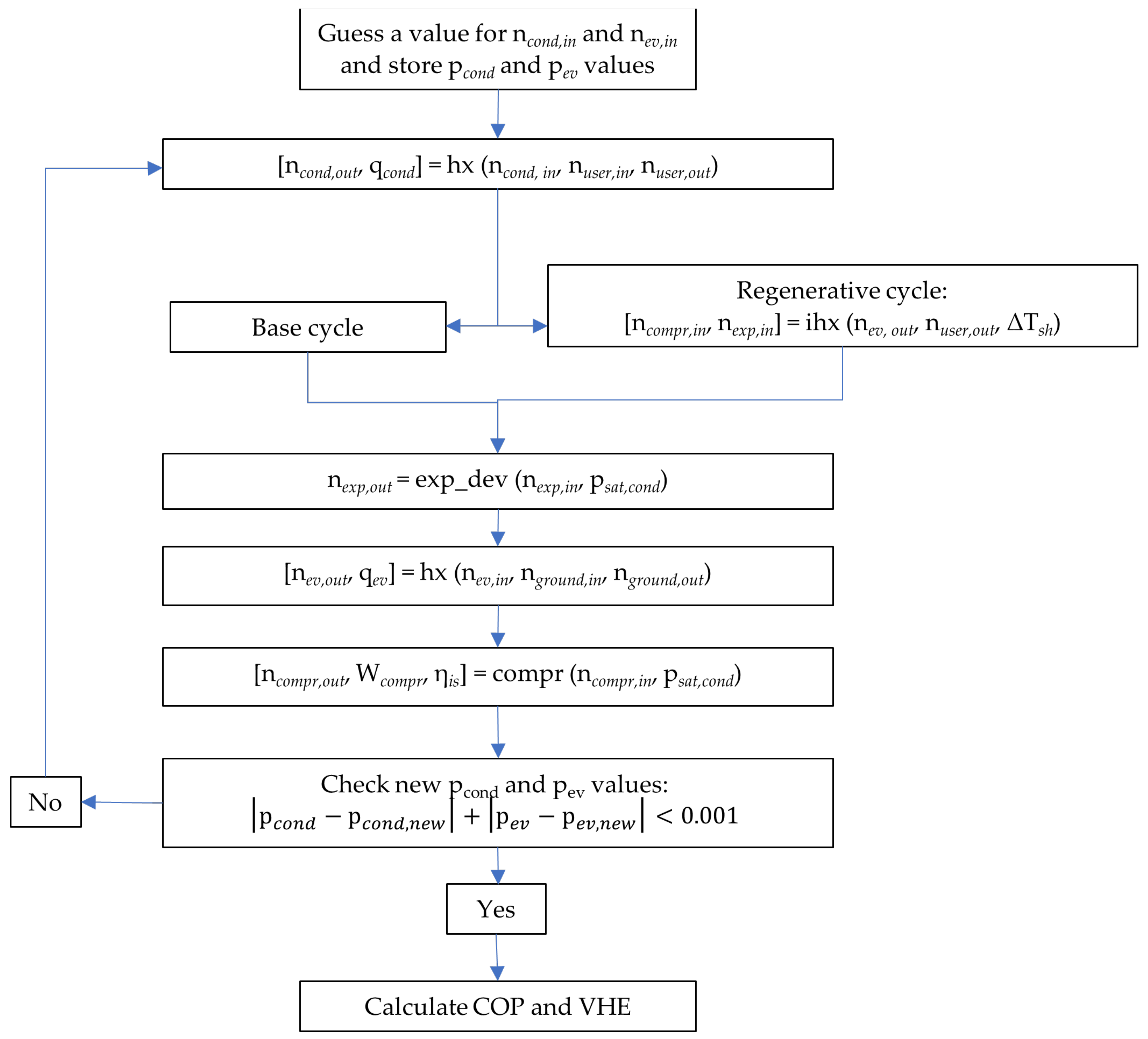
2.1. Thermodynamic Model

Each heat pump component has been implemented as a function, as described in the following sections. Every function was named after the corresponding component and reported in the present paper with the form [output1, …, outputn] = component (input1, …, inputm). In such a relationship, the first input was the thermodynamic state of the fluid at the component inlet, whereas the other inputs were particular properties requested by the refrigerant at the component outlet. The outputs were either the thermodynamic state of the fluid at the component outlet or other variables related to the component and interesting for the analysis, such as the power exchanged by the component. The symbol fref represents the REFPROP 10.0 subroutines used to calculate a certain thermodynamic property.

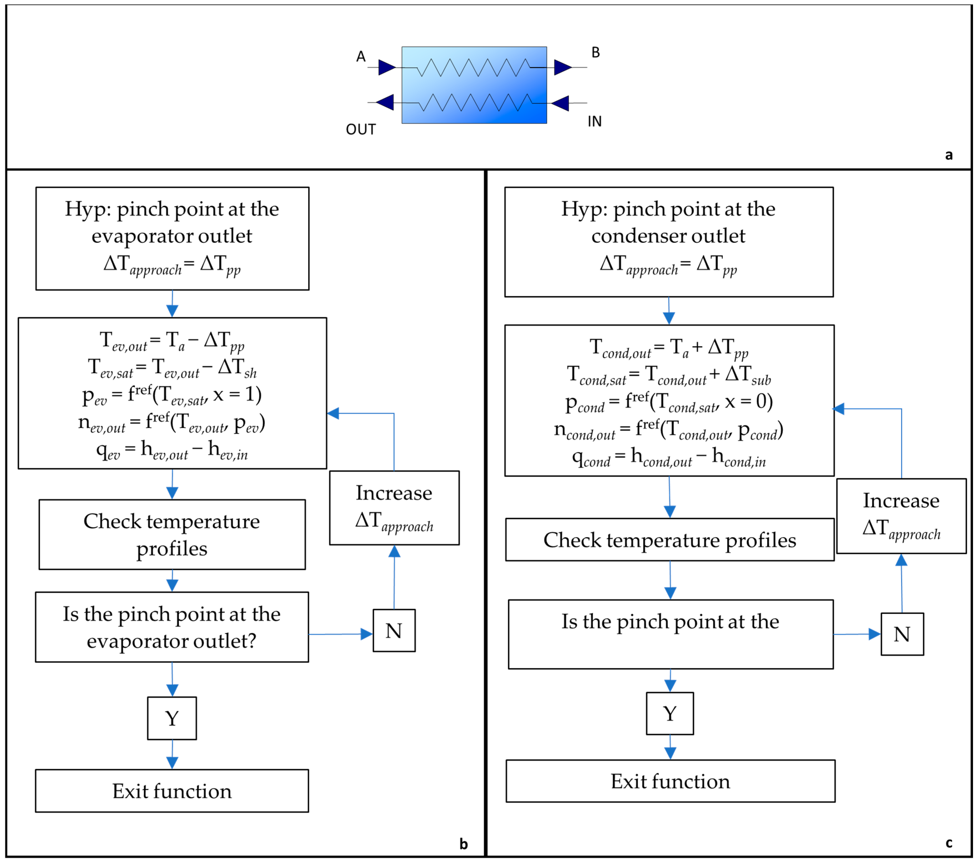
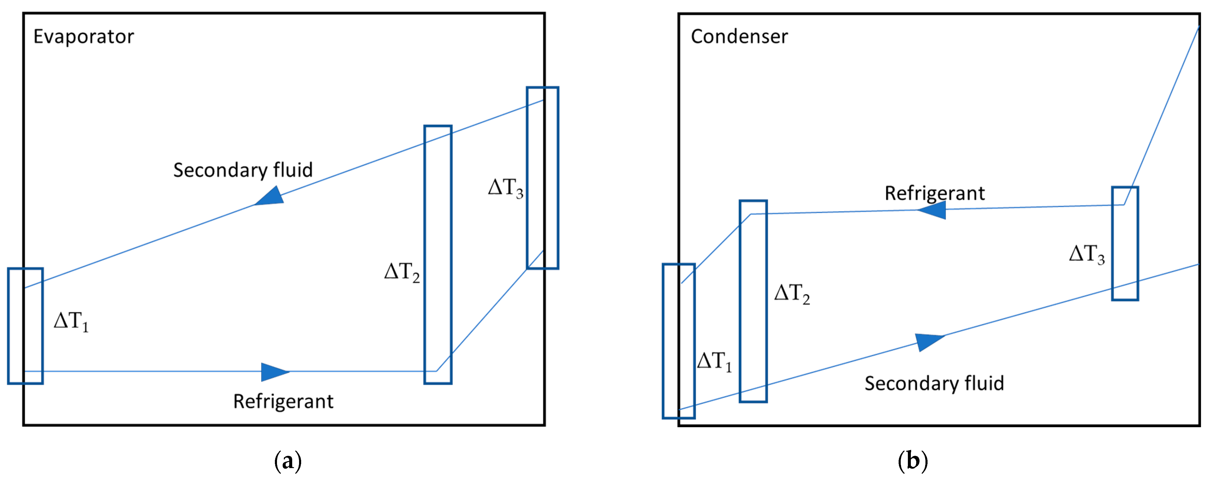
2.1.1. Evaporator and Condenser

The evaporator and condenser were modelled as shown in Figure 4a with the following function:
[nout, q] = hx(nin,na,nb)
where the subscripts in and out refer to the working fluid, whereas the subscripts a and b ports refer to the secondary circuit (see Figure 4a to visualize component ports). The symbol n represents the thermodynamic state of the fluid, i.e., an array of all the thermodynamic properties of the fluid in such a state. Superheating of 5 K was assumed at the evaporator outlet and 6 K subcooling was considered at the condenser outlet. The components were modelled through pinch point analysis considering a minimum temperature difference equal to 3 K between the refrigerant and the water temperature profiles. The output of the function was the thermodynamic state of the working fluid at the heat exchanger outlet and the cooling or heating power. The calculation was an iterative process in order to ensure no interceptions between temperature profiles, as shown in Figure 4b,c. In such a process scheme, the vapour quality xout is set equal to 0 or 1 for the condenser (saturated liquid) and the evaporator (saturated vapour), respectively. At each iteration, ∆Tapproach is increased by 0.1 K.
The temperature profiles were checked by dividing the heat exchanger into two or three sections and calculating the energy balance in particular points where the pinch point temperature difference (i.e., the minimum temperature difference between the two temperature profiles) could be violated. Considering that the refrigerant enters the evaporator as a two-phase fluid, the evaporator was divided into two sections: one between the refrigerant inlet and the saturated vapour condition and another one between the saturated vapour condition and the refrigerant outlet, where the fluid was assumed to be superheated. The condenser was divided into three sections: the first one, the desuperheating region, between the refrigerant inlet and the saturated vapour condition; the second one, the two-phase region, between saturated vapour and saturated liquid conditions; the third one, the subcooling region, between the saturated liquid condition and the refrigerant outlet. The temperature profiles were then checked through energy balances at the boundaries of such sections. Figure 5a,b illustrate the checking mechanisms for the evaporator and the condenser, respectively. On the secondary fluid side, constant specific heat and mass flow rates were assumed, such that the temperature changed linearly along the heat exchangers.

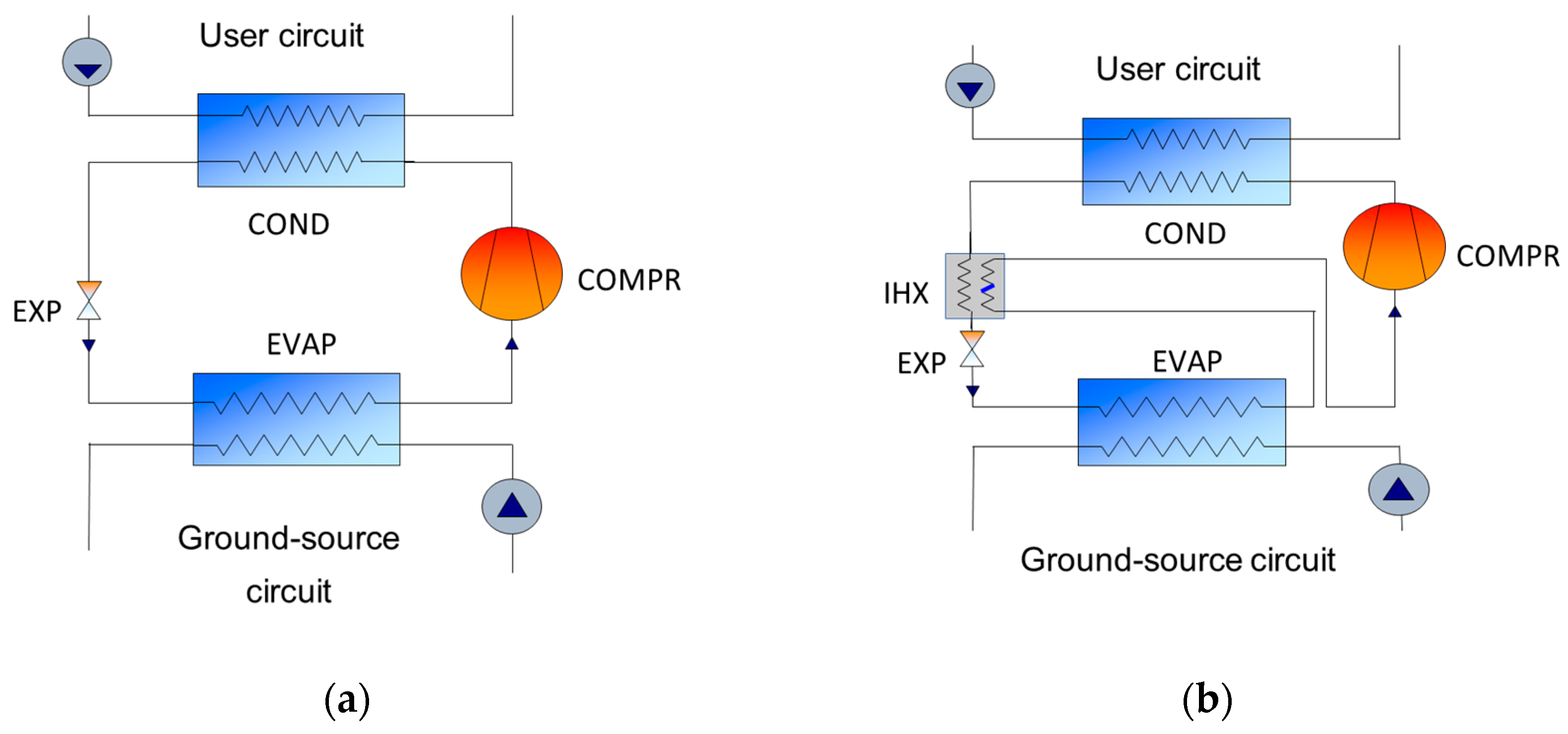
2.1.2. Internal Heat Exchanger

In the regenerative cycle, an internal heat exchanger (IHX) was added between the evaporator and the compressor. The purpose of such component was to perform the superheating outside the evaporator, in order to increase evaporating pressure and therefore increase cycle efficiency. In refrigeration, such a component is installed in order to increase the subcooling and then increase the cooling capacity. This effect was less relevant in the present work since heat pumps were considered. A fixed temperature difference was considered between the inlet and outlet of the vapour side (5 K superheating was assumed), and, consequently, the liquid side outlet entering the expansion device was calculated. Temperature profiles were not checked since the temperature difference between the vapour and the liquid line is significant in real applications. Figure 6 shows the model of the internal heat exchanger.
[ncompr,in, nexp,in] = ihx(nev,out, ncond,out)
ncompr,in = fref(pev,sat, Tev,sat + ΔTsh)
qihx = hcompr,in − hev,out
nexp,in = fref(pcond,sat, hcond,out − qihx)

2.1.3. Expansion Device

The expansion device was modelled as a simple isenthalpic pressure loss, which calculated the thermodynamic state at the outlet with inlet state and outlet pressure as inputs.
nout = exp_dev(nin, pout) = fref(hin, pout)

2.1.4. Compressor

Particular attention was paid to the modelling of the compressor due to its strong influence on the energetic analysis. To date, various models were reported to simulate the compressor depending on the assumptions made by the authors. Most of the published papers reported energetic analysis to compare several fluids used to simulate an ideal compressor with a constant isentropic efficiency equal to 1 [8,11,17]. Bobbo et al. [22] used manufacturer compressor maps to calculate the isentropic efficiency as a function of condensing and evaporating temperatures. Shen and Ally et al. [28] calculated the isentropic efficiency from manufacturer compressor maps, extending the application to refrigerants for which compressor maps were not available through a similarity criterion based on saturation pressures. The compression thermodynamic path (synthetized by the isentropic efficiency) influenced the temperature at the compressor outlet and the work performed by the compressor, thus strongly affecting the COP of the cycle. This implied that the hierarchy of the fluids in terms of energetic performance could change depending on the isentropic efficiency model applied. Thus, it was interesting to compare the effect of the various models to understand how they could influence the selection of the best alternative fluid. For this reason, several scenarios have been analysed based on isentropic efficiency. The first two (Scenarios A and B) assumed constant isentropic efficiency. Beyond the ideal case with isentropic efficiency equal to 1 (Scenario A), the assumption of constant isentropic efficiency for all the fluids considered corresponded to the case in which the compressor was optimised for each of the fluids considered. In other words, it was assumed that in optimising the compressor for a given fluid, the isentropic efficiency achievable was roughly the same as that of all the other fluids, and 0.7 (Scenario B) was considered a reasonable value in nominal working conditions. Equations (7)–(10) were used to model the compressor in Scenarios A and B.
[nout, Wcompr, ηis] = compr(nin, pout)
nout,is = fref(pout, sin)
Wcompr = (hout,is − hin)/ηis
nout = fref(pout, hin + Wcompr)
Additionally, in the previous assumption, the isentropic efficiency was assumed independently of the working conditions (the pressure ratio in particular), which is not true in reality. Then, three further scenarios, named C, D, and E, were studied, calculating the compressor-specific work using AHRI 540 (EN12900) 10-coefficient compressor maps [29]. Such maps consisted of 10 coefficient equations requiring 2 input parameters, condensing and evaporating temperatures, to calculate the power absorbed by the compressor and the mass flow rate. For the three scenarios, two different commercial compressor models were considered from the Bitzer selection software, which applied the AHRI maps:
  • 2CES-3Y: reciprocating compressor designed for R134a alternatives (compressor maps available for R134a, R1234yf, R1234ze(E), R450A, R513A, and R515B).
  • GSD60120: scroll compressor designed for R410A alternatives (compressor maps available for R410A, R32, R452B, and R454B).
Bitzer software provided a map of the performance of the selected compressors for each refrigerant that the machine is designed for and for a fixed value of superheating. It is worth noting that maps were available for all the pure compounds considered here (R134a, R1234yf, R1234ze(E), and R32). However, for some of the mixtures considered here, the coefficients were not available. In these cases, some reasonable assumptions have been made to apply the maps also to these fluids, as described below.
  • Scenario A: ideal compressor with constant isentropic efficiency equal to 1.
  • Scenario B: pseudo-ideal compressor with constant isentropic efficiency equal to 0.7.
  • Scenario C: AHRI maps were used as they were given, and the compressor work was calculated as a function of the evaporating and condensing temperatures. Compressor maps were given only for some of the analysed fluids, whereas for the newest on the market, mostly blends, compressor data were not available. In these cases, compressor maps of another fluid were considered as references. Table 3 reports the reference fluids considered. The choice was made considering the most similar fluid for which data were available for the aforementioned compressor models. In this context, three different criteria have been applied (note that a fluid for which a compressor map was available was considered a “reference fluid”, whereas an “unknown fluid” was a fluid for which a compressor map was not available):
    -
    the composition of the reference fluid was similar to that of the unknown fluid: for instance, R515B was the reference fluid for R515A;
    -
    substitutes for R134a: in case the unknown fluid was a blend, the reference fluid was the pure fluid with the higher concentration in the blend. For example, the R516A composition is R134a/R1234yf/R152a (8.5/77.5/14). Thus, R1234yf was taken as the compressor reference fluid.
    -
    substitutes for R410A: with the aim of using the same scroll compressor, if the unknown fluid was a blend, the reference fluid was assumed to be R454B, since it was the only fluid for which the compressor map was available and its thermodynamic properties (saturated pressure) were compatible with most of the alternative fluids considered.
Equations (11)–(14) were used to model the compressor in Scenario C:
[Pcompr, m] = map(Tsat,in, Tsat,in, ΔTsh)
Wcompr = Pcompr/m
nout = fref(pout, hin + Wcompr)
ηis = (hout,is − hin)/Wcompr
  • Scenario D: first, compressor maps were rearranged in order to obtain compressor isentropic efficiency maps as a function of condensing and evaporating pressures (instead of temperatures), for the refrigerants for which data were available. Then, only for the fluids with no available information about compressors, compressor maps of the baseline fluids, R134a and R410A, were considered as a reference. This solution was inspired by [29], assuming similar compressor behaviour for each fluid if the inlet pressure, the outlet pressures, and the superheating were the same, and considering a drop-in scenario. Equations (15)–(18) were used for Scenario D:
nout,is = fref(pout, sin)
ηis = map(pev, pcond, ΔTsh)
Wcompr = (hout,is − hin)/ηis
nout = fref(pout, hin + Wcompr)
  • Scenario E: the same rearrangement of the maps in terms of condensing and evaporating pressures as in scenario D was performed, but in this case considering the same fluids of Scenario C as reference fluids, instead of considering the baseline fluids (Table 3). Equations (15)–(18) are used also in this case.

2.2. Cycles Simulation

Both base and regenerative cycles have been simulated solving a series of consequential equations as shown in the flow chart of Figure 7. The system was solved iteratively by checking the convergence on the calculated saturation pressures in the evaporator and the condenser. The final outputs of the system were the coefficient of performance (COP) and the volumetric heating effect (VHE), calculated as:
COP = qcond/Wcompr
VHE = qcond∙ρev,out
If the choice of COP was straightforward, it is worth underlining the importance of the VHE as a performance indicator since it is useful to compare the size of heat pumps with the same heating capacity. Thus, the VHE has an impact on the design and the final cost of the system, which must be taken into account.
As boundary conditions, typical values for the ground source water temperature in different climatic and soil conditions in Europe [23] have been considered. These values have been coupled to typical values for the water temperatures at the user for different space heating terminals (from radiant systems to fan coils), as described below:
  • Ground-source water (or brine) temperatures (evaporator inlet): 0 °C, 3 °C, 7 °C, and 10 °C;
  • Water temperature difference between evaporator inlet and outlet: 3 °C;
  • User side water outlet temperatures (condenser outlet): 30 °C, 35 °C, 45 °C, and 55 °C;
  • Water temperature difference between condenser inlet and outlet: 5 °C.

3. Results and Discussion

Two thermodynamic cycles have been simulated considering several fluids as feasible substitutes for refrigerants R134a and R410A. In the following section, the results of such simulations are presented. Since the aim of the present work was comparing the fluid behaviour with several thermodynamic models, the following analysis was based on the relative performance indicator shown in Equations (21) and (22) and each refrigerant was compared to the high-GWP fluid to be substituted at the same boundary conditions, scenario, and thermodynamic cycle.
ΔCOP = (COPalternative − COPhighGWP)/COPhighGWP
ΔVHE = (VHEalternative − VHEhighGWP)/VHEhighGWP
where the subscript alternative refers to the new refrigerants, while high-GWP refers either to R134a or R410A. For reasons of brevity, the results have been presented only for the case of source temperature equal to 0/−3 °C (inlet/outlet) and user temperature equal to 30/35 °C (inlet/outlet).

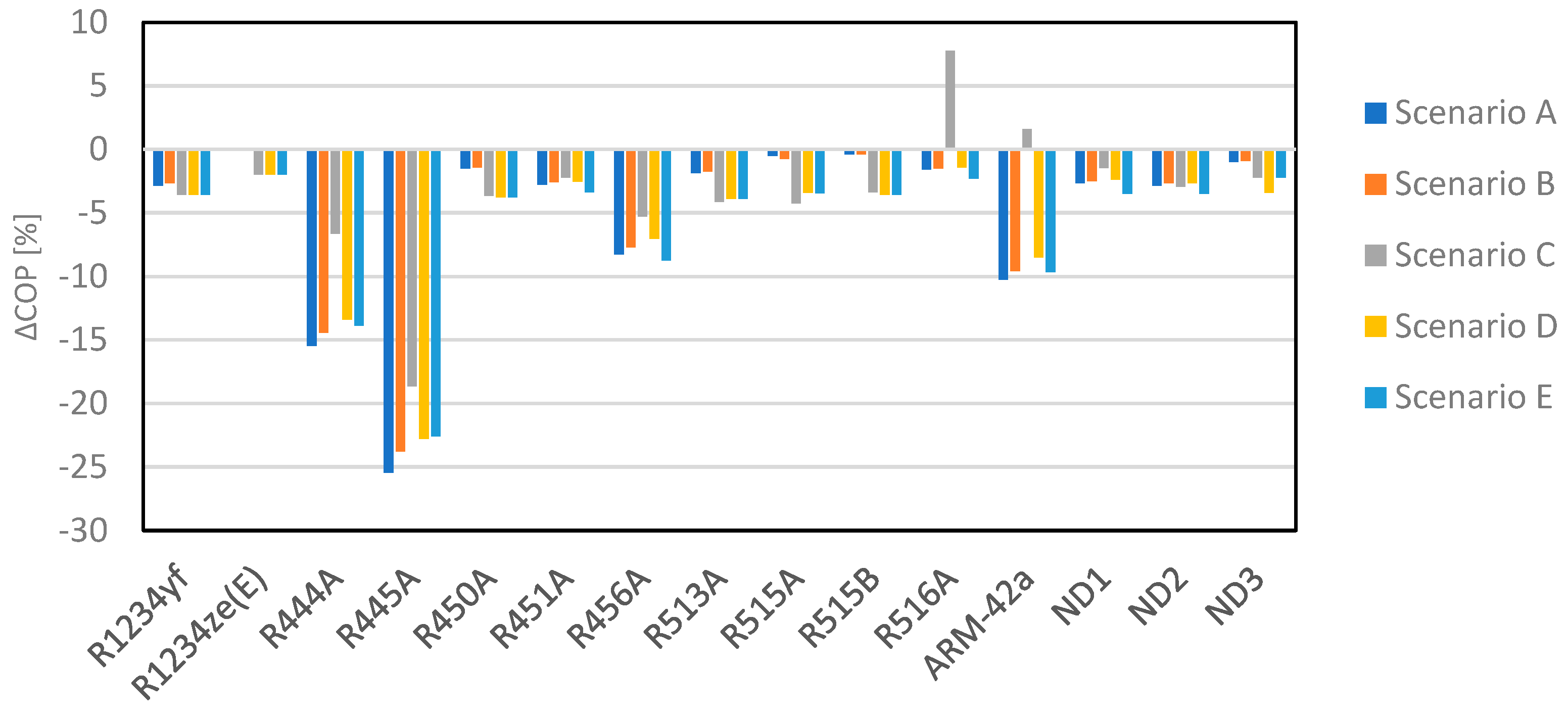
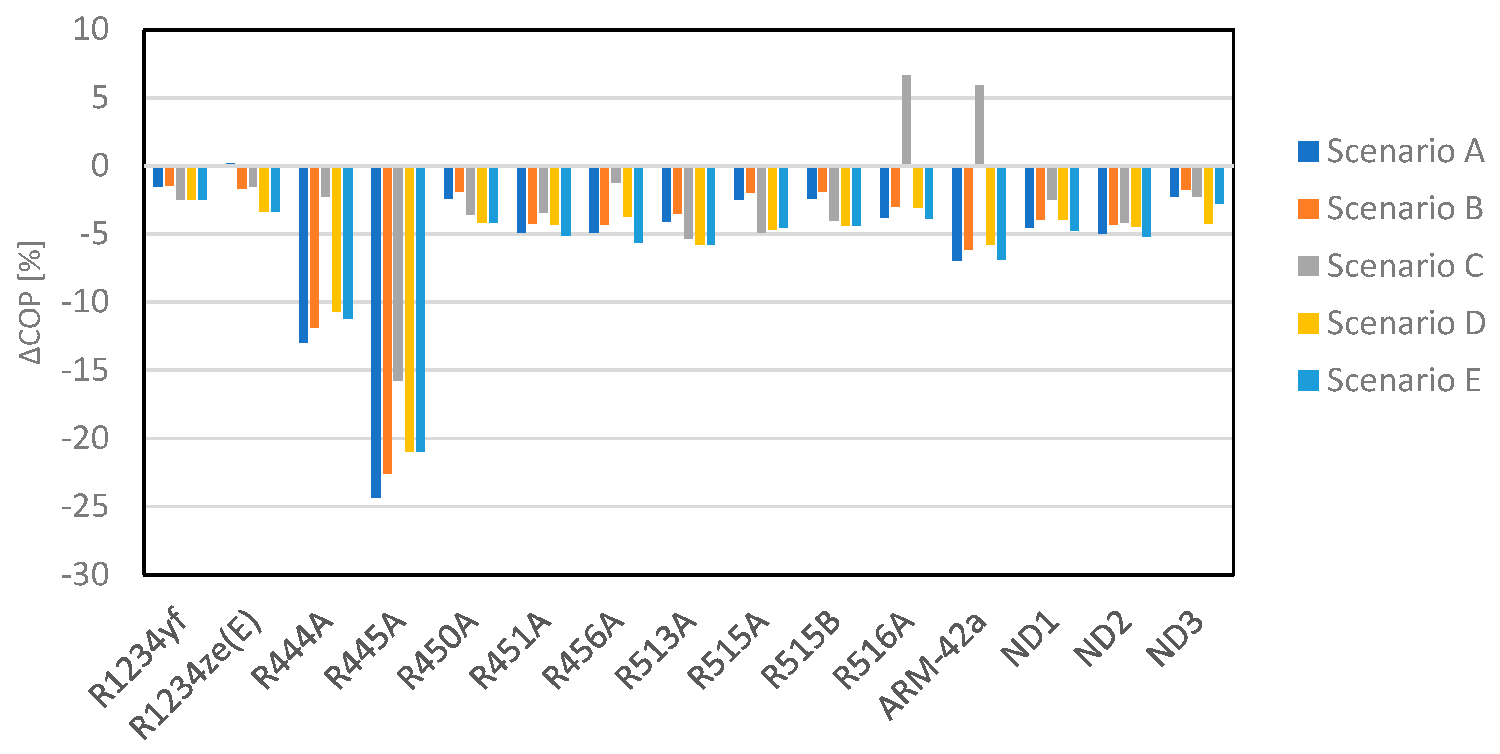
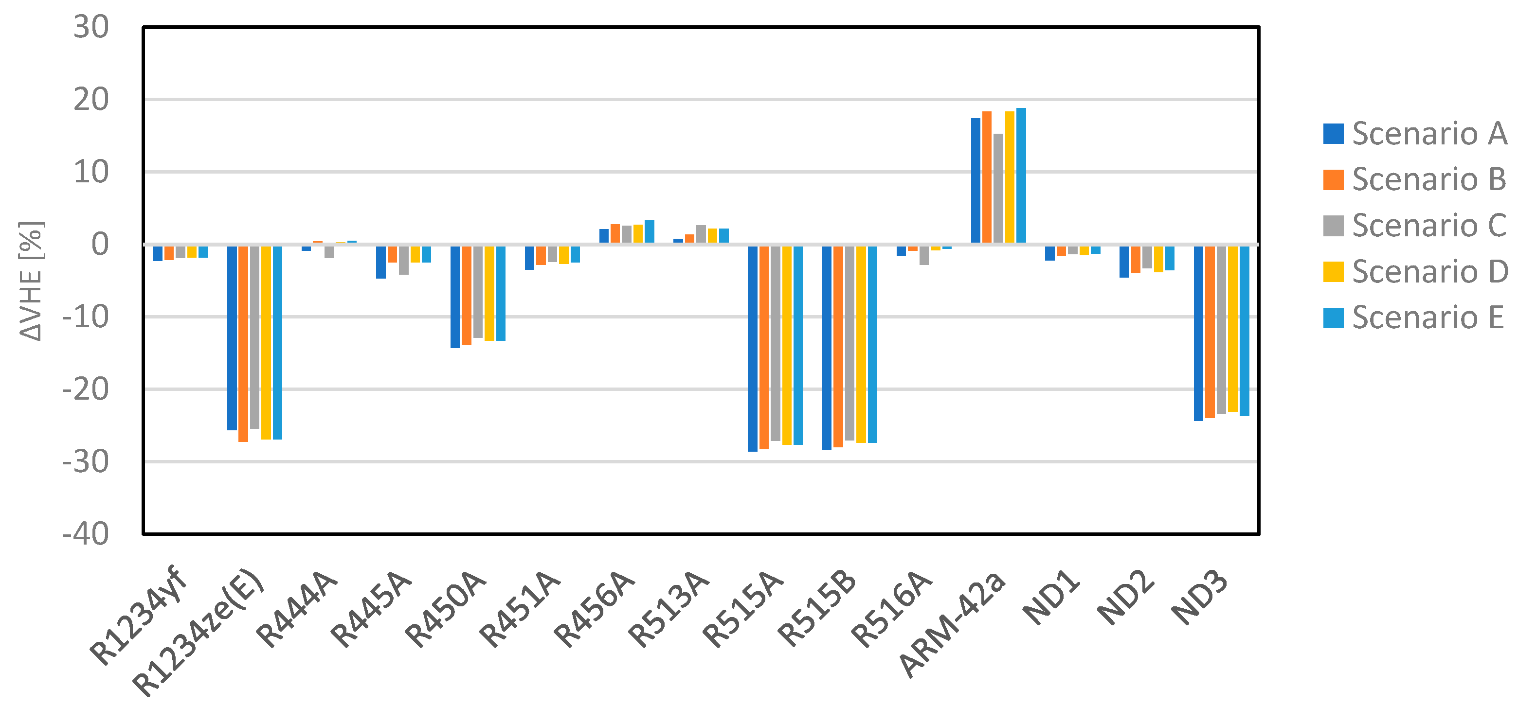
3.1. R134a and Its Alternatives

Simulation results are shown in Figure 8 and Figure 9 for the R134a substitutes, in terms of COP and VHE respectively, considering the base cycle. Figure 10 and Figure 11 are related to the regenerative cycle. On the y-axis, the relative COP (or VHE) differences between the considered fluid and the baseline fluid R134a are plotted. The same data have been reported in Tables S1–S4, respectively, of the Supporting Information.
A certain variability was noticed for each fluid among the considered scenarios in terms of both COP and VHE, even though for the last one it is lower. Such variability affected the performance ranking among fluids.
  • Base cycle: Scenarios A and B presented similar results in terms of fluids ranking. In these scenarios, R134a resulted in having the highest COP values, followed by R1234ze(E) and its blends. At the same time, R1234ze(E) and its blends, such as R515A, R515B, etc., presented VHE values from 23% to 25% lower than R134a.
As expected, the fluids, for which compressor data were available, presented almost the same results, with differences lower than 1%, for the real compressor Scenarios C, D, and E. Instead, great variability was noticed between Scenario C and the latter two, if the considered fluid had no compressor maps available. With Scenario C, R516A and ARM-42a presented COP values higher than R134a (6.5% and 1.7% respectively). Scenarios D and E presented similar results and showed R516A, R1234ze(E), ND1, ND2, and ND3 as favourite alternatives to R134a, but with a COP reduction higher than 3.5%. Among this last set of fluids, only R1234ze(E) had compressor maps available. VHE seemed to be less sensitive to the modification of the scenarios, with the exception of Scenario C for R516A and ARM-42a.
  • Regenerative cycle: the relative COP and VHE differences among alternative refrigerants and R134a presented the same trend as the base cycle. For the whole set of alternatives, except for ARM-42a, R445A, and R456A, the installation of an internal heat exchanger resulted in reducing the difference between the performance of the alternative fluid and that of R134a.
The COP variability noticed among the scenarios could be explained by the methodology applied to calculate the compressor isentropic efficiency. Figures S1–S3 (see Supporting Information) show the isentropic efficiency trend for R134a alternatives in Scenarios C, D and E respectively (in Scenarios A and B, a constant value of isentropic efficiency was assumed). In Scenario C, ARM-42a and R516A presented ηis values from 5% to 10% higher than the set of fluids for which compressor data were available, and this was reflected in the COP results. In Scenarios D and E, instead, the ηis results were similar in trends and absolute values.

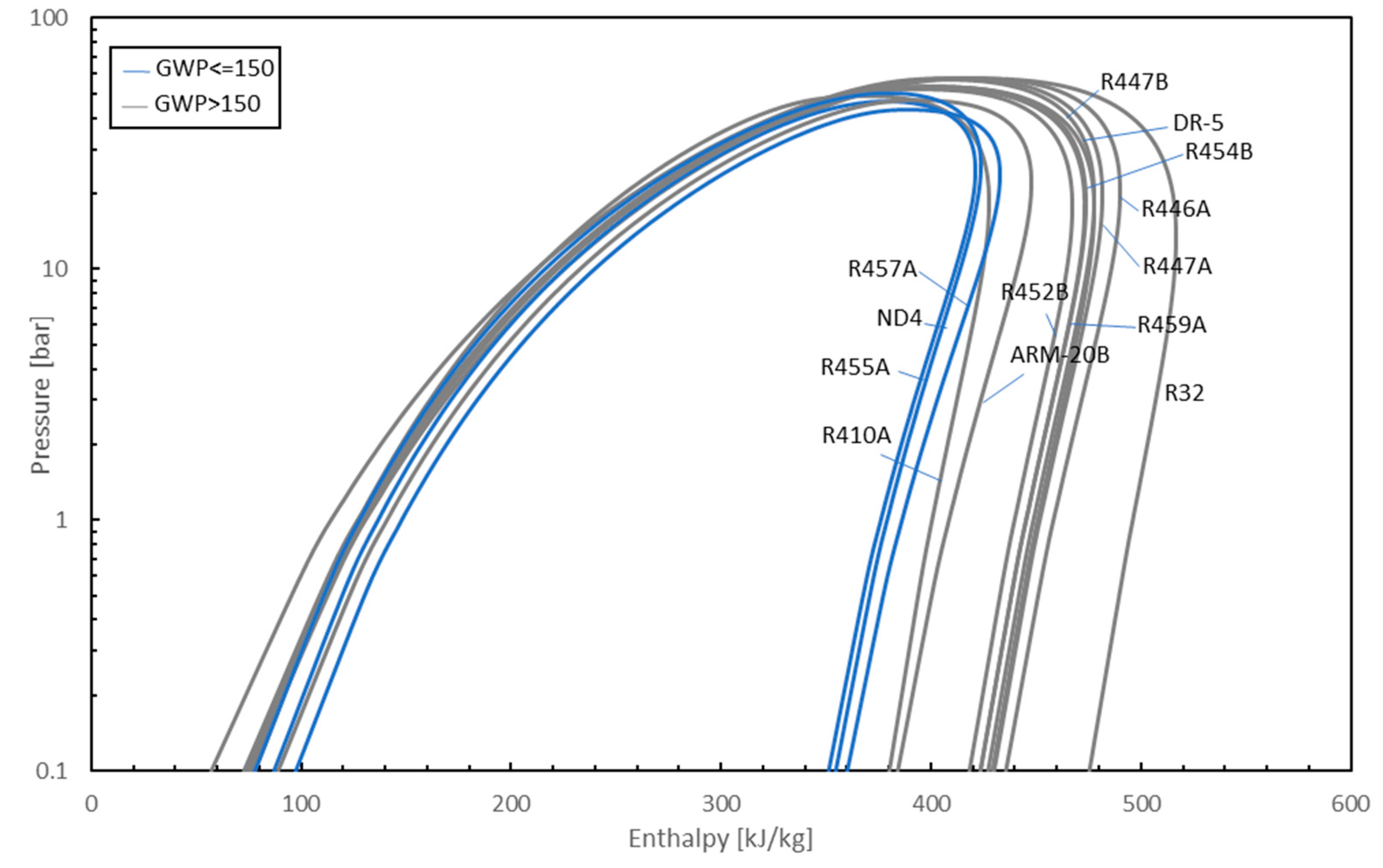
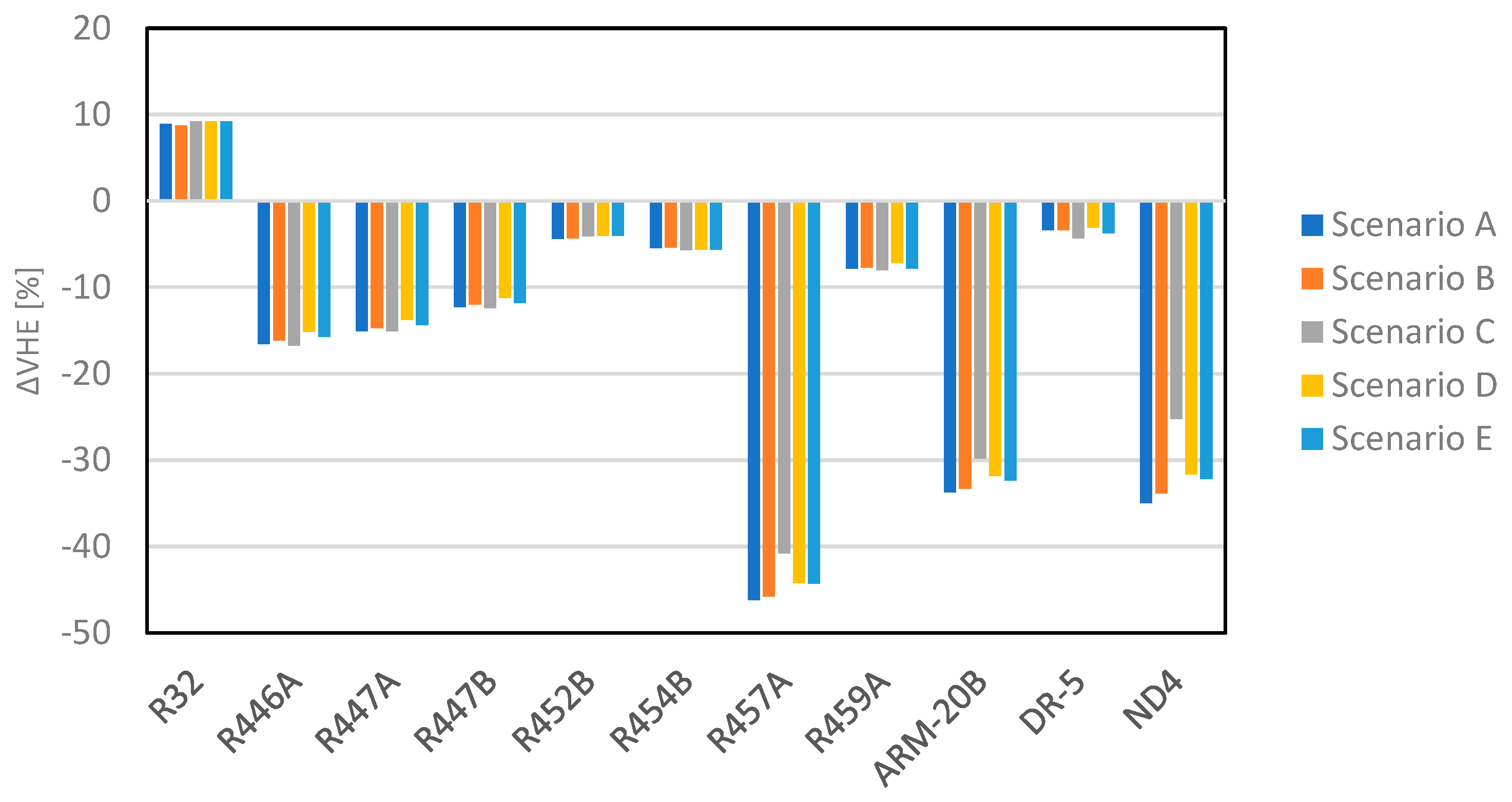
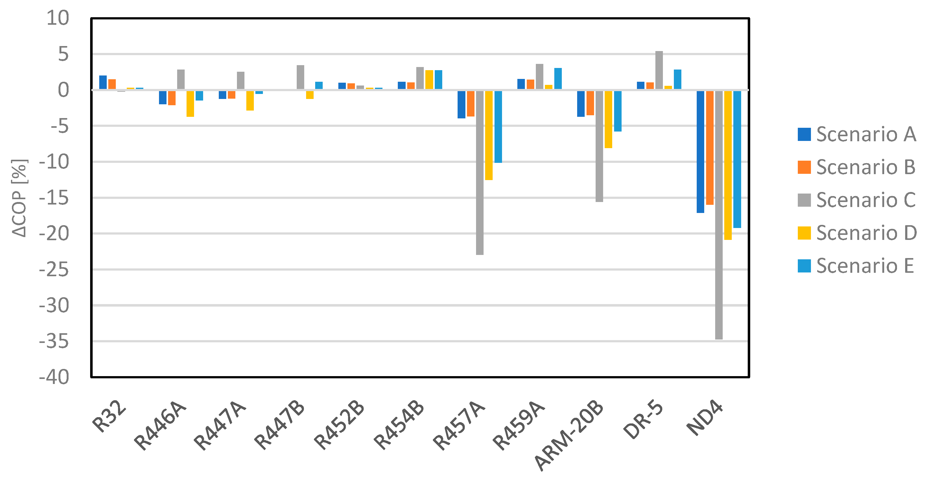
3.2. R410A and Its Alternatives

As for R134a substitutes, Figure 12 and Figure 13 show the simulation results for R410A substitutes, in terms of COP and VHE respectively, considering the base cycle. Figure 14 and Figure 15 are related to the regenerative cycle. The same data have been reported in Tables S5–S8, respectively, of the Supporting Information.
  • Base cycle: similar fluid ranking was noticed in Scenarios A and B. In such scenarios, R32 performed better than the other fluids, with an increase of 1.5% in COP and 9.9% in VHE with respect to R410A. DR-5 and R454B showed almost the same results as R410A in terms of COP (differences lower than 0.8%). In Scenario C, DR-5 and R454B showed the highest COP values (+2.9% and +0.13% with respect to R410A), but also a reduction of 7.6% and 11.8% in terms of VHE with respect to the baseline fluid. R32 had a COP reduction lower than 0.1% with respect to R410A. Scenarios D and E showed similar results among fluids, but no difference in fluid performance ranking with respect to scenarios A and B. In Scenario E, R32, R454B, and also DR-5 presented COP values similar to R410A with a relative difference lower than 0.5%. A lower sensibility to the chosen scenario was noticed on VHE.
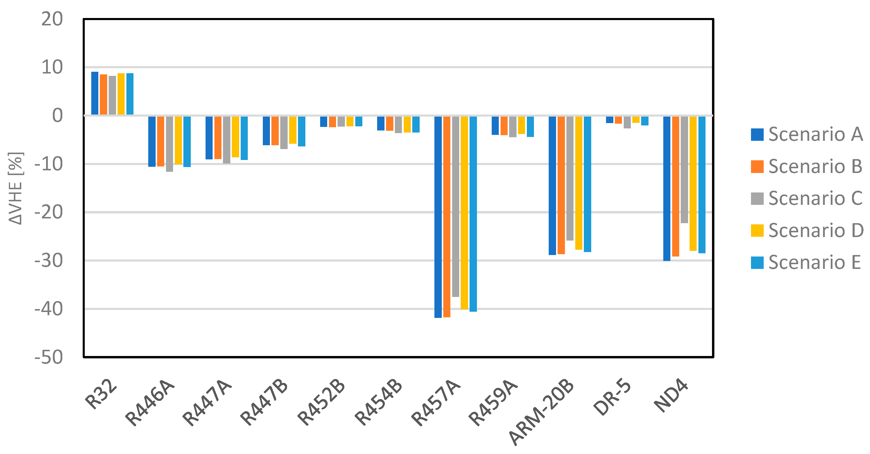
  • Regenerative cycle: the relative COP and VHE differences among R410A and its potential substitutes presented the same trend of the base cycle. With Scenarios A and B, the modification of the base cycle asserted a greater benefit for R459A, DR-5, R454B, and R452B performance in terms of COP with respect to R410A. Instead, in scenarios C, D, and E, the COP difference between R410A and its alternatives decreased, with respect to the base cycle, for all the alternatives. In particular, in Scenario C, R457A, ARM-20B, and ND4 were the only alternatives with COP values lower than R410A. No significant differences were noticed between the base and regenerative cycles in terms of the relative VHE difference between R410A and its alternatives.
Such results may find an explanation for the compressor isentropic efficiency calculation (see Figures S4–S6 for Supporting Information), as seen for R134a. Important differences could be noticed for Scenario C, which were reflected in the COP calculation with the advantage of DR-5 and R459A and the disadvantage of ARM-20B, R457A and ND4. A lower variability was then noticed for Scenarios D and E.

4. Sensitivity Analysis

In order to better explain the previous results, a sensitivity analysis of the thermodynamic model to the isentropic efficiency has been conducted. Such analysis was based on Scenario B and the base cycle since the isentropic efficiency was set as a constant and not calculated. Equation (23) has been considered and explained in the Supporting Information.
dCOP d η i s = h o u t , e v h o u t , c o n d h o u t , c o m r , i s h o u t , e v
From Equation (23), the COP was sensitive to isentropic efficiency through a factor dependent only on the fluid and the boundary conditions. Figures S7 and S8 (see Supporting Information) show the calculated sensitivity coefficients for the R134a and R410A substitutes, respectively, for several user outlet temperatures and for a source temperature of 0/−3 °C (inlet/outlet). The influence of isentropic efficiency on COP was greater at higher user outlet temperatures (and consequently higher condensing pressure). In any case, such influence was relevant. For instance, considering a user temperature of 30/35 °C (inlet/outlet) and a source temperature of 0/−3 °C (inlet/outlet), a change in the isentropic efficiency from 0.60 to 0.65 caused a COP increase of 0.182 for R134a and 0.177 for R410A. Hence, this difference was capable of modifying the performance ranking and altering the choice of the best alternative refrigerant.

5. Conclusions

The present paper aimed to individuate interesting low-GWP alternatives to R134a and R410A and, at the same time, to discuss the methodology of such analysis. An energetic analysis has been conducted on two sets of potential substitutes for R134a and R410A considering two thermodynamic cycles: a base cycle and a regenerative cycle. Five scenarios have been studied focusing on the evaluation of the compression isentropic efficiency: two scenarios with constant isentropic efficiency equal to 1 (Scenario A) and equal to 0.7 (Scenario B), and three scenarios (C, D, and E) with variable isentropic efficiency, on the base of compressor maps given by manufacturers, as reported in AHRI 540 (EN 12900). In particular, a scroll compressor has been considered for R410A substitutes, and a reciprocating compressor has been taken into account for R134a substitutes. In Scenario C, the compressor maps have been implemented as they were given, so that the isentropic efficiency was a function of fluid, evaporating temperature, condensing temperature, and superheating at the compressor inlet. Since not all the simulated fluids had compressor maps available, being mostly mixtures new on the market, a similarity criterion was applied to assign the compressor maps available for a known refrigerant to such fluids. In Scenarios D and E, the compressor maps of the available refrigerants were refitted to calculate isentropic efficiency as a function of condensing and evaporating pressures, instead of temperatures. Scenarios D and E differed from each other when fluids with no compressor available were involved: in the former scenario, compressor maps of the baseline fluids (R134a and R410A) were considered, whereas, in the latter scenario, the same similarity criterion as Scenario C was used to select the compressor maps. The comparison among the alternative fluids and scenarios was based on the increase (or decrease) in the coefficient of performance (COP) and the volumetric heating effect (VHE) with respect to R134a and R410A.
As a relevant influence was observed for compression isentropic efficiency on COP values, a sensibility analysis was conducted to study the influence of such parameters on the COP. Considering the thermodynamic model applied in this work, the sensibility coefficient dCOP/(dη_is) depended on the fluids and the boundary conditions of the simulation. This coefficient was greater for lower differences between condensing and evaporation pressures. For instance, a change in the isentropic efficiency from 0.60 to 0.65 caused an increase of 0.182 in the COP for R134a and 0.177 for R410A, considering 0/−3 °C as inlet/outlet source temperatures and 30/35 °C as inlet/outlet user temperatures, whereas the increase was about 0.112 for R134a and 0.106 for R410A when moving to inlet/outlet user temperatures of 50/55 °C.
It was noticed that Scenarios A, B, D, and E had similar rankings among the alternative fluids in terms of relative values for both COP and VHE with respect to the R134a and R410A. Instead, Scenario C showed several exceptions enlightening some fluids as the best- or worst-performing ones with relative differences higher than expected. It is worth noting that such exceptions regarded those refrigerants for which no compressor maps were available and for which a similarity criterion was applied: thus, the assumptions made for Scenario C were probably less reliable than those for the other scenarios. Examples of this were R516A and ARM-42a as R134a alternatives, which presented isentropic efficiencies from 5% to 10% higher than the average of the set, or ARM-20B, R457A, and ND4 as R410A alternatives which showed isentropic efficiencies up to 30% lower than the average of the set. Thus, some critical issues arose when a similarity criterion was based on refrigerants composition and the calculation of isentropic efficiency was based on evaporation and condensation temperatures, whereas a good agreement was noticed when isentropic efficiency was calculated from evaporation and condensation pressures even though a similarity criterion based on refrigerants composition was applied. In synthesis, the assumption of a constant isentropic efficiency was acceptable when different fluids were compared to define their performance ranking. If one’s purpose is to evaluate the absolute performance of the refrigerants depending on the boundary conditions, scenarios D or E were more suitable, since these represented more realistically the fluid behaviour, also in the case of fluids for which no compressor data were available. Scenario C was less reliable in representing the real behaviour of fluid not represented by the manufacturer maps. On the basis of these observations, refrigerants such as R1234ze(E), R515A, R515B, and R516A were the most promising R134a alternatives if the base cycle was considered, and the zeotropic mixtures R450A and ND3 could be included in these if the regenerative cycle was considered. Regarding R410A alternatives, R32, R454B, and DR-5 were the most promising fluids, and R459A could be included if the regenerative cycle was considered.
Further research will be carried out including new promising refrigerants once their equations of state are available, and the compressor maps will be updated once these will be available for the refrigerants considered in the present work.

Supplementary Materials

The following supporting information can be downloaded at: https://www.mdpi.com/article/10.3390/en16093757/s1.

Author Contributions

Conceptualization, D.M. (Davide Menegazzo) and S.B.; methodology, D.M. (Davide Menegazzo) and S.B.; investigation, D.M. (Davide Menegazzo), S.B., A.B., L.F., F.P., A.T., M.D.C., L.C., G.M., D.M. (Dimitris Mendrinos); writing, D.M. (Davide Menegazzo); supervision, A.B., L.F. and S.B.; project administration, A.B., L.F., S.B., M.D.C., L.C., F.P., A.T., D.M. (Dimitris Mendrinos), G.M. All authors have read and agreed to the published version of the manuscript.

Funding

This work has been financially supported by the EU project GEO4CIVHIC, which is gratefully acknowledged by the authors. The project has received funding from the European Union’s Horizon 2020 research and innovation program under grant agreement No. 792355. Energies 16 03757 i001

Institutional Review Board Statement

Not applicable.

Informed Consent Statement

Not applicable.

Data Availability Statement

Not applicable.

Conflicts of Interest

The authors declare no conflict of interest.

References

  1. Nowak, T.; Westring, P. European Heat Pump Market and Statistics Report. In The European Heat Pump Association; AISBL (EHPA): Brussels, Belgium, 2018. [Google Scholar]
  2. United Nations. Paris agreement. In Proceedings of the Conference of the Parties to the United Nations Framework Convention on Climate Change, Paris, France, 30 November–12 December 2015. [Google Scholar]
  3. Menegazzo, D.; Lombardo, G.; Bobbo, S.; De Carli, M.; Fedele, L. State of the Art, Perspective and Obstacles of Ground-Source Heat Pump Technology in the European Building Sector: A Review. Energies 2022, 15, 2685. [Google Scholar] [CrossRef]
  4. Council, E. Directive 2010/31/EU of the European Parliament and of the Council of 19 May 2010 on the energy performances of buildings. Off. J. Eur. Union 2010, 153, 13–35. [Google Scholar]
  5. Directive (EU) 2018/844 of the European Parliament and of the Council of 30 May 2018 amending Directive 2010/31/EU on the Energy Performance of Buildings and Directive 2012/27/EU on Energy Efficiency. Available online: https://eur-lex.europa.eu/legal-content/EN/TXT/PDF/?uri=CELEX:32018L0844&from=EN (accessed on 9 December 2020).
  6. Sanner, B.; Dumas, P.; Gavriliuc, R.; Zeghici, R. The use of geothermal energy for buildings refurbishment in Europe-technologies, success stories and perspectives. Rev. Romana Ing. Civ. 2013, 4, 183. [Google Scholar]
  7. Directive (EU) 2014/517 of the European Parliament and of the Council of 16 April 2014 on fluorinated greenhouse gases and repealing Regulation (EC) 2006/842. Available online: https://www.eea.europa.eu/policy-documents/regulation-eu-no-517-2014 (accessed on 19 April 2023).
  8. Mota-Babiloni, A. Analysis of Low Global Warming Potential Fluoride Working Fluids in Vapour Compression Systems. Experimental Evaluation of Commercial Refrigeration Alternatives. Ph.D. Thesis, Jaume I University, Castellón de la Plana, Spain, 2016. [Google Scholar]
  9. Bobbo, S.; Di Nicola, G.; Zilio, C.; Brown, J.S.; Fedele, L. Low GWP halocarbon refrigerants: A review of thermophysical properties. Int. J. Refrig. 2018, 90, 181–201. [Google Scholar] [CrossRef]
  10. Makhnatch, P.; Khodabandeha, R. The role of environmental metrics (GWP, TEWI, LCCP) in the selection of low GWP refrigerant. Energy Procedia 2014, 61, 2460–2463. [Google Scholar] [CrossRef]
  11. Mota-Babiloni, A.; Navarro-Esbrı, J.; Barragan-Cervera, A.; Moles, F.; Peris, B. Analysis based on EU Regulation No 517/2014 of new HFC/HFO mixtures as alternatives of high GWP refrigerants in refrigeration and HVAC systems. Int. J. Refrig. 2015, 52, 21–31. [Google Scholar] [CrossRef]
  12. Thu, K.; Takezato, K.; Takata, N.; Miyazaki, T.; Higashi, Y. Drop-in experiments and exergy assessment of HFC-32/HFO-1234yf/R744 mixture with GWP below 150 for domestic heat pumps. Int. J. Refrig. 2021, 121, 289–301. [Google Scholar] [CrossRef]
  13. Lee, Y.; Kang, D.; Jung, D. Performance of virtually non-flammable azeotropic HFO1234yf/HFC134a mixture for HFC134a applications. Int. J. Refrig. 2013, 36, 1203–1207. [Google Scholar] [CrossRef]
  14. Llopis, R.; Sánchez, D.; Cabello, R.; Catalán-Gil, J.; Nebot-Andrés, L. Experimental analysis of R-450A and R-513A as replacements of R-134a and R-507A in a medium temperature commercial refrigeration system. Int. J. Refrig. 2017, 84, 52–66. [Google Scholar] [CrossRef]
  15. Aprea, C.; Greco, A.; Maiorino, A. Comparative performance analysis of HFO1234ze/HFC134a binary mixtures working as a drop-in of HFC134a in a domestic refrigerator. Int. J. Refrig. 2017, 82, 71–82. [Google Scholar] [CrossRef]
  16. Yang, Z.; Feng, B.; Ma, H.; Zhang, L.; Duan, C.; Liu, B.; Zhang, Y.; Chen, S.; Yang, Z. Analysis of lower GWP and flammable alternative refrigerants. Int. J. Refrig. 2021, 126, 12–22. [Google Scholar] [CrossRef]
  17. Heredia-Aricapa, Y.; Belman-Flores, J.; Mota-Babiloni, A.; Serrano-Arellano, J.; García-Pabón, J.J. Overview of low GWP mixtures for the replacement of HFC refrigerants: R134a, R404A and R410A. Int. J. Refrig. 2020, 111, 113–123. [Google Scholar] [CrossRef]
  18. Devecioğlu, A.G.; Oruç, V. Energetic performance analysis of R466A as an alternative to R410A in VRF systems. Eng. Sci. Technol. Int. J. 2020, 23, 1425–1433. [Google Scholar] [CrossRef]
  19. Godwin, D.; Ferenchiak, R. The implications of residential air conditioning refrigerant choice on future hydrofluorocarbon consumption in the United States. J. Integr. Environ. Sci. 2020, 17, 29–44. [Google Scholar] [CrossRef] [PubMed]
  20. Kunz, O.; Klimeck, R.; Wagner, W.; Jaeschke, M. The GERG-2004 Wide-Range Equation of State for Natural Gases and Other Mixtures; U.S. Department of Energy Office of Scientific and Technical Information: Washington, DC, USA, 2007.
  21. Bertsch, S.; Groll, E.A. Two-stage air-source heat pump for residential heating and cooling applications in northern U.S. climates. IJR 2008, 31, 1282–1292. [Google Scholar] [CrossRef]
  22. Bobbo, S.; Fedele, L.; Curcio, M.; Bet, A.; De Carli, M.; Emmi, G.; Poletto, F.; Tarabotti, A.; Mendrinos, D.; Mezzasalma, G.; et al. Energetic and Exergetic Analysis of Low Global Warming Potential Refrigerants as Substitutes for R410A in Ground Source Heat Pumps. Energies 2019, 12, 3538. [Google Scholar] [CrossRef]
  23. Aisyah, N.; Alhmaid, M.I.; Nasruddin, S.; Lubis, A.; Saito, K. Parametric study and multi-objective optimization of vapor compression heat pump system by using environmental friendly refrigerant. J. Adv. Res. Fluid Mech. Therm. Sci. 2019, 54, 44–56. [Google Scholar]
  24. GEO4CIVHIC—Most Easy, Efficient and Low Cost Geothermal Systems for Retrofitting Civil and Historical Buildings. Topic LCE-17-2017, Type of Action IA, Call H2020-LCE-2017-RES-IA. Available online: www.geo4civhic.eu (accessed on 19 April 2023).
  25. Van Rossum, G.; Drake, F.L., Jr. Python Reference Manual; Centrum voor Wiskunde en Informatica: Amsterdam, The Netherlands, 1995. [Google Scholar]
  26. Lemmon, E.; Bell, I.; Huber, M.; McLinden, M.O. NIST Standard Reference Database 23, “Reference Fluid Thermodynamic and Transport Properties (REFPROP), Version 10.0”; National Institute of Standards and Technology: Gaithersburg, MD, USA, 2018.
  27. ANSI/ASHRAE 34-2019; Designation and Safety Classification of Refrigerants. ASHRAE: Peachtree Corners, GA, USA, 2019.
  28. Shen, B.; Ally, M. Energy and Exergy Analysis of Low-Global Warming Potential Refrigerants as Replacement for R410A in Two-Speed Heat Pumps for Cold Climates. Energies 2020, 13, 5666. [Google Scholar] [CrossRef]
  29. EN 12900:2013; Refrigerant compressors—Rating Conditions, Tolerances and Presentation of Manufacturer’s Performance Data. Commission Regulation: Brussels, Belgium, 2013.
Figure 1. Comparison of the saturation curves for the studied alternatives for R134a.
Energies 16 03757 g001
Figure 2. Comparison of the saturation curves for the studied alternatives for R410A.
Energies 16 03757 g002
Figure 3. Simplified thermodynamic scheme of (a) base cycle and (b) regenerative cycle.
Energies 16 03757 g003
Figure 4. (a) Functional scheme of the heat exchanger. (b) Iterative process for the evaporator. (c) Iterative process for the condenser.
Energies 16 03757 g004
Figure 5. Demonstration of the method applied for checking the temperature profile agreements for (a) the evaporator and (b) the condenser.
Energies 16 03757 g005
Figure 6. Functional scheme of the internal heat exchanger.
Energies 16 03757 g006
Figure 7. Simulation flow chart for both base and regenerative cycle.
Energies 16 03757 g007
Figure 8. Relative comparison on COP for R134a alternatives with the base cycle [user temperature: 30 °C/35 °C (inlet/outlet), source temperature: −3 °C/0 °C].
Energies 16 03757 g008
Figure 9. Relative comparison on VHE for R134a alternatives with the base cycle [user temperature: 30 °C/35 °C (inlet/outlet), source temperature: −3 °C/0 °C].
Energies 16 03757 g009
Figure 10. Relative comparison on COP for R134a alternatives with the regenerative cycle [user temperature: 30 °C/35 °C (inlet/outlet), source temperature: −3 °C/0 °C].
Energies 16 03757 g010
Figure 11. Relative comparison on VHE for R134a alternatives with the regenerative cycle [user temperature: 30 °C/35 °C (inlet/outlet), source temperature: −3 °C/0 °C].
Energies 16 03757 g011
Figure 12. Relative comparison on COP for R410A alternatives with the base cycle [user temperature: 30 °C/35 °C (inlet/outlet), source temperature: −3 °C/0 °C].
Energies 16 03757 g012
Figure 13. Relative comparison on VHE for R410A alternatives with the base cycle [user temperature: 30 °C/35 °C (inlet/outlet), source temperature: −3 °C/0 °C].
Energies 16 03757 g013
Figure 14. Relative comparison on COP for R410A alternatives with the regenerative cycle [user temperature: 30 °C/35 °C (inlet/outlet), source temperature: −3 °C/0 °C].
Energies 16 03757 g014
Figure 15. Relative comparison on VHE for R410A alternatives with the regenerative cycle [user temperature: 30 °C/35 °C (inlet/outlet), source temperature: −3 °C/0 °C].
Energies 16 03757 g015
Table 1. Studied substitutes for R134a.
FluidCompositionGWP100Tcrit
[°C]
Pcrit
[bar]
Tglide
[K]
ASHRAE Safety Class [27]
R134a 1430101.0640.59 A1
R1234yf 494.733.82 A2L
R1234ze(E) 7109.3636.35 A2L
R444AR152a/R32/R1234ze(E) (5/12/83)91106.3644.789.5A2L
R445AR134a/R1234ze(E)/CO2 (9/85/6)135106.0445.4422A2L
R450AR134a/R1234ze(E) 42/58605104.4738.220.65A2L
R451AR134a/R1234yf (10.2/89.8)14994.3634.430.05A2L
R456AR32/R134a/R1234ze(E) 6/45/49687102.6641.754.57A2L
R513AR134a/R1234yf (44/56)63194.7836.32 A1
R515AR1234ze(E)/R227ea (88/12)393108.6135.66 A1
R515BR1234ze(E)/R227ea (91.1/8.9)293108.8835.84 A1
R516AR134a/R1234yf/R152a (8.5/77.5/14)14296.6436.15 A2L
ARM-42aR152a/R134a/R1234yf (11/7/82)6493.739.044.9A2L
ND1 [12]R134a/R1234yf (15/85)21894.2834.710.06A2L
ND2 [12]R134a/R1234yf (5/95)7594.5134.120.04A2L
ND3 [14]R134a/R1234ze(E) (10/90)14994.3734.420.4A2L
Table 2. Studied substitutes for R410A.
FluidCompositionGWP100Tcrit
[°C]
Pcrit
[bar]
Tglide
[K]
ASHRAE Safety Class [26]
R410AR32/R125 (50/50)208871.3449.010.12A1
R32 67578.1157.820A2L
R446AR32/R600/R1234ze(E) (29/3/68)47085.9557.254.47A2L
R447AR32/R125/R1234ze(E) (68/3.5/28.5)58385.357.114.08A2L
R447BR32/R125/R1234ze(E) (68/8/24)71083.5556.443.48A2L
R452BR32/R125/R1234yf (67/7/26)67777.0552.21.17A2L
R454BR32/R1234yf (68.9/31.1)46678.1052.671.33A2L
R457AR32/R1234yf/R152a (18/70/12)13990.0543.086.67A2L
R459AR32/R1234yf/R1234ze(E) (68/26/6)46079.5553.61.88A2L
ARM-20BR32/R1234yf/R152a (35/55/10)25185.2547.215.76A2L
DR-5R32/R1234yf (72.5/27.5)49078.0253.31.09A2L
ND4 [11]R32/R1234yf/CO2 (22/72/6)15184.9549.814.19A2L
Table 3. Reference fluids for the compressor maps.
Compressor Reference Fluid Compressor Reference Fluid
Simulated FluidsScenarios C and EScenario DSimulated FluidsScenarios C and EScenario D
R134aR134aR134aR410AR410AR410A
R1234yfR1234yfR1234yfR32R32R32
R1234ze(E)R1234ze(E)R1234ze(E)R446AR454BR410A
R444AR1234ze(E)R134aR447AR454BR410A
R445AR1234ze(E)R134aR447BR454BR410A
R450AR450AR450AR452BR452BR452B
R451AR1234ze(E)R134aR454BR454BR454B
R456AR450AR134aR457AR454BR410A
R513AR513AR513AR459AR454BR410A
R515AR515BR134aARM-20BR454BR410A
R515BR515BR515BDR-5R454BR410A
R516AR1234yfR134aND4R454BR410A
ARM-42aR1234yfR134a
ND1R1234yfR134a
ND2R1234yfR134a
ND3R1234ze(E)R134a
Disclaimer/Publisher’s Note: The statements, opinions and data contained in all publications are solely those of the individual author(s) and contributor(s) and not of MDPI and/or the editor(s). MDPI and/or the editor(s) disclaim responsibility for any injury to people or property resulting from any ideas, methods, instructions or products referred to in the content.

