
CFD-Based Sensitivity-Analysis and Performance Investigation of a Hydronic Road-Heating System

1
Institute of New Energy Systems, Technische Hochschule Ingolstadt, Esplanade 10, 85049 Ingolstadt, Germany
2
Department of Chemical Sciences, University of Padova, Via Marzolo 1, 35141 Padova, Italy
3
Technical Infrastructure Planning, I/P2-434 Audi AG, 85045 Ingolstadt, Germany
*
Authors to whom correspondence should be addressed.
Energies 2023, 16(5), 2173; https://doi.org/10.3390/en16052173
Submission received: 21 December 2022
/
Revised: 4 February 2023
/
Accepted: 8 February 2023
/
Published: 23 February 2023
(This article belongs to the Special Issue Modelling of Energy-Efficient Industrial and Environmental Processes Using Computational Fluid Dynamics (CFD))
Abstract
:To minimize the impact of snowfall and ice formation on safety of transportation, salt is sprinkled on the asphalt every winter. However, the use of salt has economical as well as ecological disadvantages. To resolve these problems, road heating systems are used in the northern regions of Europe and America. Despite their widespread usage, considerable potential of the operational optimization is evident. The current systems are controlled under predefined weather conditions such as start of operation at 5 °C air temperature, even when snowfall is absent. Consequently, loss of energy input to heat the system is caused. To avoid unnecessary financial and energetic expense, this study presents CFD-based performance investigation as a basis for a novel predictive controller to increase the operational efficiency of hydronic road heating systems (HRS). The simulation model was developed based on a real operational HRS located in Ingolstadt and composed of bridges and ramps for a total surface of 1989 m2. Climate data of the years 2019–2020 from local weather stations were implemented in the simulation model for performance prediction on extreme climate conditions. This investigation identified that up to 70% of operational hours in terms of energy input can be saved by using a hypothetical predictive controller, thus making the HRS a more economically efficient and environmentally attractive alternate to conventional de-icing techniques.
1. Introduction
Unsafe driving conditions can be created by snow accumulation and ice formation on road surfaces. The typical method to have free road surfaces is to sprinkle salts and sand as part of winter maintenance. The use of salts and sand has three main goals: anti-compaction of snow, de-icing, and anti-icing of the surface of the roads [1]. The anti-icing agents are used to prevent the wet roads from freezing, the de-icing products are used to melt the existing ice/snow on the road surface, and, finally, the anti-compaction processes are phenomena for preventing the snow from compacting into a hard crust [2]. However, use of salts and sands can result in ground and surface water pollution [3] as well as in causing the corrosion of road infrastructure and vehicles [4]. Additionally, the usage of the combination of salts and sand has certain temperature limitations. The Scandinavian countries follow a lower limitation of −8 °C at the road surface for using the salt and sand mixture [5]. A more environmentally friendly method for road maintenance to avoid unsafe winter roads is to use strategies based on thermal analysis of the involved systems. The thermal approach involves the transfer of heat to warm the road surface to melt the ice and snow. The method is valid not only for ice/snow prevention but also for friction control [6].
Generally, hydronic road-heating systems (HRSs) include a network of pipes, which are embedded in the pavement of the road. Thermal energy is transferred into the road/pavement by circulation of warm fluid in the pipes. Among the types of heat, the most used are waste heat from industrial processes, heat from electric resistance, and geothermal heat. Usually, renewable energy sources are preferred in order to minimize the impact of HRSs [7]. Temperature measurements of the heat-transfer fluid in the pipe network are crucial to regulate the amount of heat flux transferred to the road/pavement along the surface area of the pipe and thereby to determine the working conditions on the surface. HRSs avoid the formation of unsafe conditions on road surfaces, which can be caused by water condensation. Thus, the physical–chemical parameters related to the condensation process need to be investigated with the aim to reduce the energy consumption required by the HRSs [8].
Special consideration must be applied to the near real-time energy demands, so that a control system is required to correlate the HRSs to the local energy sources, such as a geothermal heat pump [7]. Several control systems have been suggested. Li et al. [9] studied two types of controllers: a simple ON/OFF controller working at a constant value of thermal energy to transfer, and a dynamic controller with the possibility to vary the amount of heat to use. The variable warming system was applied to a bridge and was characterized by an inverse heat-conduction process along the thickness of the bridge. Both controllers succeeded in maintaining the bridge surface at a temperature higher than 0.5 °C. However, comparing the two types of controllers, the system working at a constant heat value (206 W/m2) consumed approximately 34% more energy than the dynamic heating system (maximum required heat power was ca. 150 W/m2). A different scenario was suggested by Pahud [10,11], who considered the air temperature with respect to regulating the HRS. The system was set to heat only when the air temperature was between +4 °C and −8 °C. Indeed, below −8 °C the amount of water vapor in the air is very low and the probability of ice formation at the road surface is almost negligible [12]. Another approach were the simulation models suggested by Abbasi [13], who considered two situations to activate the HRS: in the first one, the surface temperature is lower than 0 °C, while in the second on the surface temperature is lower than both 0 °C and the dew-point temperature. Simulations showed that the controller also considering the dew-point temperature allowed to save 10 times the annual required energy for hydronic road heating. Mirzanamadi et al. [14] selected the type of controller based on a surface temperature below both 0 °C and the dew-point temperature and defined a temperature threshold between +0.1 °C and +1.6 °C as both the freezing temperature and the dew-point for pre-heating the road surface. The addition of the temperature threshold and of the pre-heating process was very efficient in terms of decrement of slippery conditions at road surfaces [12].
The focus of the present paper is to describe the development of an optimized control algorithm for a rigorous utilization of the required energy for de-icing and de-snowing of road surfaces. The algorithm is based on actual/forecasted weather conditions and suggests a valid improvement to the real system of the Ingolstadt case study, which is automatically activated when ambient temperature falls below 5 °C, even if there are negligible risks of snowfall/ice formation. On-site weather stations and weather forecasts from the German Weather Service are to be fed into the controller via an internet connection. The controller algorithm will process the incoming data feed and set the heating system according to the situational requirements instead of predefined ON/OFF logic.
2. Methodology
In this paper, a real operating hydronic road-heating system located in the city of Ingolstadt in the southern part of Germany was used as case study to develop a simulation model. The model has the final aim to optimize the operational conditions in terms of energy cost and environmental sustainability. A CFD investigation provides the basis to develop a novel control algorithm to regulate the existing and new HRS. First of all, the geometric morphology and the numerical dimensions of the Ingolstadt HRS were used to draw the system. Then the drawing was imported into the CFD platform. Two main parameters were analyzed, i.e., the temperature of the asphalt on the road surface and the time interval required to reach and maintain an average temperature of 3 °C at the asphalt surface. The simulations were carried out considering three weather conditions, i.e., when the temperature of the air is −6 °C, −4 °C, and −2 °C. Additionally, the model was used in three different scenarios, i.e., when the initial temperature of the asphalt is 3 °C, 0 °C, and −3 °C with snowfall. The results of the simulation model were correlated to the experimental data to compare the theory with the reality. To reduce the uncertainty, the base CFD model was optimized with the implementation of more precise boundary conditions and a calibration process. Validation of the model was obtained for a wide range of parameters. Finally, a prototype of a predictive controller for the HRS was developed and tested on-site for performance analysis. It is evident that working parameters need to be tailored for the specific heating applications. CFD offers an efficient tool to improve the overall performances of the system, i.e., lower power consumption with higher heating capacity.
3. Structure of the Ingolstadt HRS
The Ingolstadt HRS consists of three bridges and corresponding connecting ramps. The system was built in 2017 for entry and exit automotive traffic management of a parking space with an overall thermally activated surface area of 1989 m2. The system is located in the north-western district of the city with location coordinates of N 48.79512, E 11.40415. Figure 1 shows an aerial view of the parking space with the three thermally activated bridges. The detailed technical specifications of the system are described in the following sections. Additional information is reported in Ahmed et al. [15].
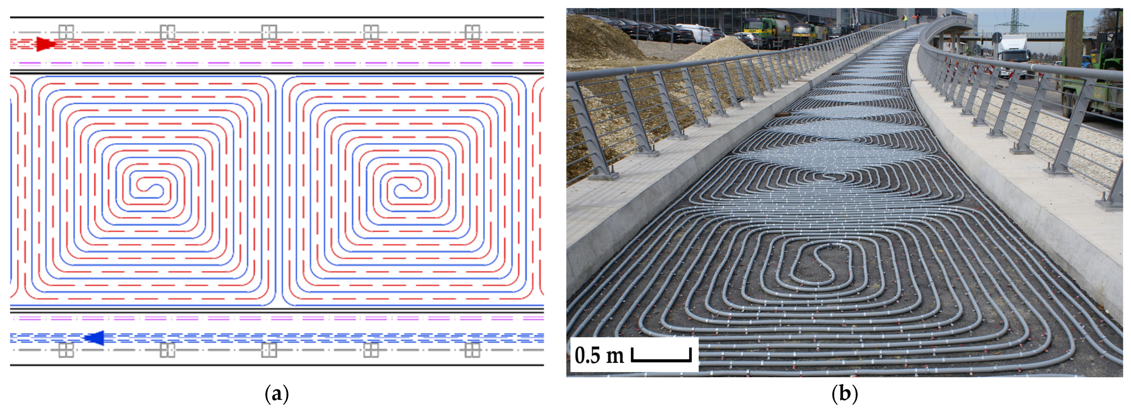
Ingolstadt HRS consists of a total of 144 heating circuits embedded in asphalt. A distribution box is located every six heating circuits to maintain a uniform flow rate of the heat-transfer fluid and temperature inside the pipe system. Twenty-four boxes with a heat capacity of 500 kW distribute the heating from a nearby industrial installation to the pipe system. To cover extreme winter events, an additional heat pump with a total heating capacity of 300 kW is also integrated. Heating circuits are made of aluminum-coated PE-Xa SDR11 pipe registers. The laying pattern of the pipe registers is illustrated in Figure 2.
Table 1 shows the length of bridge and connecting ramps for all sections of the HRS and details of heating circuits embedded in each part. Each heating circuit activates an area of ca. 14 m2.
The structure of the road consists of three layers of MA 8S-type asphalt. The bottom layer is mastic asphalt installed above a stone and gravel foundation, which is concrete in the case of the bridges. It has a thickness of 3 cm. On this layer, the heating pipe circuit is laid down in patterns and fixed using screws and clamps. This heating circuit is embedded in a second layer of asphalt with a thickness of ca. 4 cm. The top layer consists of 3 cm of rolled asphalt so that the total thickness of the asphalt layer is ca. 10 cm. Figure 3 shows a cross-section of the road with the embedded pipe arrangement.
The heating circuit consists of an oxygen-tight polyethylene PE-Xa SDR11-type pipe with a wall thickness of 2.4 mm and an internal diameter of 20 mm. The pipe has an aluminum coating with a thickness of 0.1 mm to increase the mechanical and physical–chemical stability. This metal–plastic composite pipe has operating temperatures between −40 °C and +95 °C and is temperature-resistant to up to the 250 °C it is exposed to during the installation of asphalt. It is very stable to notching and stress cracking. The geometric pattern of the heating circuit is characterized by a laying distance of 10 cm between the pipes.
The heat-transfer medium inside the pipe system is Coracon Geko AF-8. This fluid contains 14.6% of denatured ethanol (100% made from plants), it is completely biodegradable, and it has a significantly lower viscosity compared to heat-transfer fluids containing glycol (up to −58%). The frost protection is adjusted to −8 °C while the flash point is 42 °C. The three sections of the Ingolstadt HRS are filled with a total of 9470 L of Geko AF-8.
A series of sensors are installed on-site to determine the climate conditions of the air (wind speed and direction, relative humidity, pressure, temperature) and process operations of the heat-transfer fluid. The data are acquired every 10 min and stored in a central control unit.
In order to monitor the surface temperature, IRS31 pro-UMB intelligent passive road-surface sensors were installed. These sensors can measure the temperatures between −40 °C to +80 °C with an accuracy of ±0.2 °C. Furthermore, the accuracy is increased to ±0.1 °C for the temperature range between −20 °C to +20 °C. Figure 4 shows the installed sensor in sector exit North.
An average value of the gathered data is automatically computed by the central control station. The estimated error caused during transfer of data from the sensors to the central control station is automatically calculated and adjusted with the data measured by the control unit.
Operational data of the heating system are collected, which include the mass flow rate of the ecological heat-transfer fluid and the outlet and inlet temperature. Several pressure sensors are located along the local heating pipes, to regulate and maintain adequate operational conditions. The Ingolstadt HRS is automatically activated as soon as the ambient temperature falls below 5 °C and then reaches a thermal stabilization, irrespective of precipitation. Thus, the system is heating even if there are negligible risks of snowfall, snow accumulation, or ice-formation. On the contrary, as illustrated in the following sections, the optimized system operates only under the condition that there is high risk of snowfall/ice-formation and accumulation. The developed optimized control algorithm allows to reduce energy costs.
4. Computational Simulation Model
Three major stages are considered to develop the CFD simulation model for sensitivity analysis and performance investigation of the HRS under operational conditions: firstly, the design of the geometry of the heating circuit via computer-aided design (CAD) software, then, the choice and implementation of the physical models and solvers, and finally, the mesh generation.
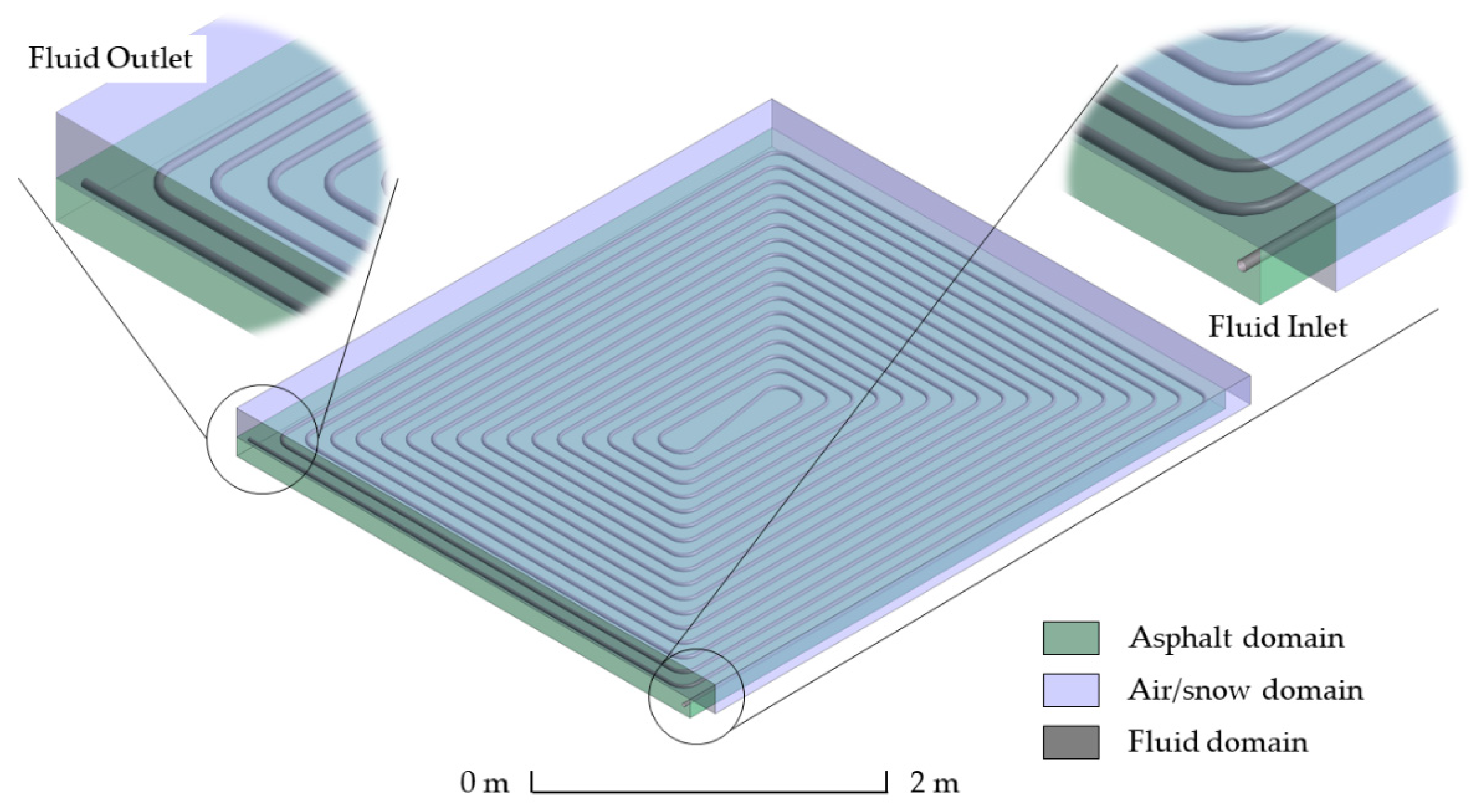
The 3D-CAD drawing for CFD simulations was created using the commercial software ANSYS Design Modeler. Geometric dimensions and material parameters of the heating circuit were modelled using an asphalt domain with a length of 3.8 m and a width of 3.4 m, i.e., an area of actual heating circuits of ca. 13 m2. The air domain—i.e., air flowing above the asphalt surface—had a height of 15 cm. The fluid domain—i.e., the actual pipes made up of PE-Xa with aluminum coating—was designed inside the asphalt domain as shown in Figure 5. All dimensions of the pipe component such as distance between the tubes, bending radius, number of turns, and depth inside the asphalt were used without down-scaling.
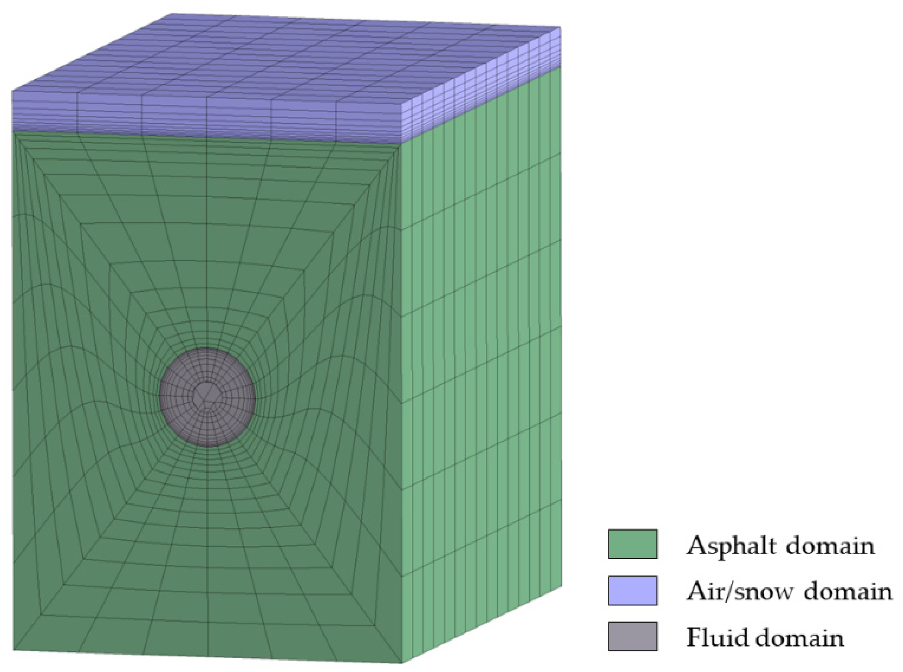
The commercial software ANSYS Mesher was used to generate a mesh of the model volumes and surfaces. Hexahedral meshing was implemented for this analysis as, in comparison to the typical tetrahedral mesh, the hexahedral mesh provides higher solution accuracy, numerical stability, and less diffusivity. Hexahedron-shaped element layers were generated to create the mesh of the asphalt volume. A grid was generated for the asphalt volume of 1.9 m3. For the wall boundaries, i.e., the asphalt around the tubes of the pipe system, the geometry was split into four sweepable parts. Sub-divisions were defined alongside each edge of sweepable parts. Furthermore, inflation layers with a growth rate of 1.5 per layer and first-layer thickness of 0.02 mm were defined in the direction of pipes and on the surface of the asphalt in the air domain, as visible in Figure 6. The surface mesh was swept through the geometry with 15 subdivisions. This created an almost pure hexahedral mesh.
The simulation model contains a total of 3.4 × 10⁶ nodes and 4 × 10⁶ elements. Quality and type of mesh discretization of the three different domains are decisive for model accuracy. Furthermore, the computational simulation speed is inversely proportional to the complexity of the mesh. To not exceed the requirements of high calculation capacity and memory resources, a balance between simulation speed and accuracy was analyzed. Using the base and calibrated model, several initial variants of meshes were simulated. These included coarse, medium-quality, high-quality, and finest-quality meshes. Analysis showed that the error between simulation and measured data for high-quality and finest-quality mesh was extremely low. However, the time required, i.e., computational power consumption, was approx. 25% higher for finest-quality mesh compared to medium-quality mesh. A compromise was achieved using several mesh resolutions in the different model domains. In this respect, the number of cells was limited to four million and varying-size cells were specifically created in different volumes and on surfaces.
The mesh was imported into the commercial software ANSYS Fluent. Simulation was set up using energy equation and laminar-type model. Regarding the CFD simulations, the solar radiation and respective heat transfer were considered. ANSYS Fluent provides several radiation models, which allow to include radiation, with or without a participating medium, in heat-transfer simulations. In addition, a solar load model can be used to include the effects of solar radiation in the simulations. The Rosseland radiation model [16] is suggested as implementation alongside solar ray tracing. Indeed, in comparison to the other radiation models, the Rosseland model is faster, requires less memory, and can be used for optically thick media, such as the current HRS. For the Rosseland model the pressure-based solver was used. Actual longitude and latitude of the HRS site in Ingolstadt were defined for solar calculator. Table 2 shows the properties of materials from ANSYS database [17] used for simulation.
To model the heat transfer, two coupled-wall type interfaces were created: the fluid–solid interface between pipe tube and asphalt and the fluid–solid interface between asphalt surface and air/snow layer on asphalt.
The Green–Gauss cell-based gradient was used as solution method and second-order upwind spatial discretization was implemented for momentum, energy, turbulent kinetic energy, dissipation rate, and intermittency.
The main assumptions applied to the computational simulation model are the following:
- A fully developed velocity profile is in the pipe volume;
- A constant average mean velocity is along the pipe volume;
- Components of fluid velocity which are normal to the axis of pipe are assumed negligible;
- Heat transfer from the fluid in the pipe to the outside occurs only in radial direction;
- All three layers of asphalt are modelled as one domain with pipe profiles embedded;
- Heat transfer to the bottom and sides of the asphalt domain is negligible because of the thermal insulation.
In order to analyze the temperature distribution profile for heat-transfer processes inside the pipe, the partial differential equation (PDE) in the cylindrical coordinate system can be written as follows [18]:
where (Kelvin) is the temperature of the coolant at a given part of the pipe, kf is the thermal conductivity of the ethanol-based fluid (0.5 W/m·K), ρw is its density (975 kg/m3), cp is its heat capacity (3891 J/kg·K), vs (m/s) is its velocity, and Qw is the induced heat source though the pipe wall. Similarly, the heat transfer through asphalt can be described as follows [18]:
where ρa is the asphalt density (2120 kg/m3), is the heat capacity (920 J/kg·K), Ta (Kelvin) is the temperature, ka is the thermal conductivity (0.7 W/m·K), and Qw is the induced heat source due to heat transfer in HRS [18].
5. Results and Discussion
5.1. Model Calibration and Validation
The process of calibration and validation of the simulation model determines if the computational simulation agrees with the physical reality. It demonstrates the accuracy of CFD code, so that it may be used with the credence that credible results will be extracted using sensitivity analysis. This section presents the validation of the model by comparing the asphalt surface temperature obtained with the model and the on-site temperature sensors. The respective weather and operational data from these time slots were implemented into the CFD model and computational value of asphalt surface temperature were obtained. Table 3 presents the weather conditions registered from October 2019 to April 2020 in terms of air temperature and wind speed, together with the operational parameter of the HRS in terms of fluid inlet temperature and asphalt surface temperature. The Ingolstadt HRS is activated when the ambient temperature falls below 5 °C. Then the system reaches a thermal stabilization. Therefore, for each case in Table 3, the asphalt surface temperature is the equilibrium surface temperature obtained from the sensors located along the HRS and contains the most critical data points of the entire season such as highest and lowest wind speeds. In the last two columns of Table 3 the results from the CFD simulations are presented using the starting (base) and optimized (final) model (see next sections for the explanation of the two models) to calculate the asphalt surface temperature.
For the simulation process, the respective values of solar radiation and irradiation were obtained from the Baumannshof–Manching weather station (Station ID 15632) operated by the German Weather Service [19]. The station is located approximately 10 km south of Ingolstadt city. These climate data are open source. The respective radiation values were integrated into the computational model for validation and verification purposes. Average asphalt surface temperature deviated strongly from measured data in the first model, i.e., base model. The base model was then calibrated to narrow the error range between values. The major design modifications were as follows:
- Height of fluid domain above asphalt was increased to 25 cm from the initial value of 2.5 cm used in the base model;
- The inlet of the fluid domain was extended by 25 cm before the start of the asphalt domain, while in the base model it was coincident with the asphalt.
Thus, the velocity profile required an initial distance to fully develop and results from the base model were obtained with ±6% error. To avoid these effects, the inlet of the fluid domain was sufficiently extended so that the velocity profile is fully developed when the asphalt-fluid interface begins. It reduced the error percentage to ±2%. Figure 7 shows the comparison between the asphalt surface temperatures obtained measuring the HRS in Ingolstadt and using the final calibrated CFD model.
5.2. Scenarios to Reach an Asphalt Surface Temperature of 3 °C
At the Ingolstadt HRS an asphalt surface temperature of 3 °C is considered the numerical value to activate the heating system inside the pipe circuits. Therefore, this value was implemented in the CFD models and the period of time required to reach the average asphalt surface temperature of 3 °C under specific weather conditions was calculated in the CFD simulations. The calculated time period was used to set the start of the operation of the HRS to before the predicted forecast of snowfall/ice formation were known based on weather conditions.
Since the weather conditions significantly influence the time period required to reach and maintain the average temperature of 3 °C on the asphalt surface, a sensitivity analysis was performed to determine the effect of the theoretically worst weather conditions. The analysis was made by varying the parameter of the real air temperature and the initialization conditions. Figure 8 shows the temperature contours on the asphalt surface in case of snowfall/ice formation forecast implemented in the CFD model.
For all simulations, mass flow rate and inlet temperature of the heat-transfer fluid were fixed at 8.53 × 10⁻³ kg/s and 22.5 °C, respectively. The velocity-inlet type boundary condition was used as heat-transfer fluid; thus, the mass flow rate of 8.53 × 10⁻³ kg/s corresponded to 0.27 m/s inlet velocity. The velocity of wind was fixed at 10 m/s. For this study, the weather conditions on 4 December 2019 at 11:00 AM were selected, because during December climate conditions are comparatively colder with lower temperatures as well as lower-than-average values of direct and diffuse solar irradiation. Historical data from the Baumannshof–Manching weather station shows direct solar irradiation of 500 W/m2 and diffuse solar irradiation of 350 W/m2. For the solar load calculator, a fair-weather condition was implemented with a sunshine factor of 1. The sunshine factor is a useful indicator for the computed incident load that accounts for a reduction in direct solar irradiance that can penetrate because of shielding due to cloud cover or similar events. A sunshine factor of 1 refers to the theoretical maximum solar irradiation. The HRS is initially turned off, i.e., there is no circulation of heat-transfer fluid inside the pipe circuits. The term initialization at a specific temperature is used in the present paper to indicate that the temperature of the asphalt domain including pipe tubes is set at that temperature at the beginning of the CFD simulation process, i.e., when the HRS has started operations. In the following, three scenarios are presented as case studies, i.e., with initialization at 3 °C, 0 °C, and −3 °C with snowfall. The time interval required to reach and maintain the average temperature of 3 °C on the surface of the asphalt is calculated at each initialization condition when the ambient air temperature is −6 °C, −4 °C, and −2 °C.
5.2.1. Initialization at 3 °C
The analysis of the temperature values obtained from the sensors installed on-site suggests that under usual weather conditions, the average asphalt surface temperature is most frequently between 3 °C and 6 °C before the HRS starts to work. Figure 9 shows the time interval required to reach and maintain a temperature of 3 °C on the surface of the asphalt when the initialization is set at 3 °C.
The profiles in Figure 9 suggest that to be operational the HRS requires only 41.200 s, i.e., approx. 11 h and 27 min before forecasted snowfall or ice formation at an ambient temperature of −6 °C.
5.2.2. Initialization at 0 °C
According to the field data of the sensors, an average asphalt surface temperature between 0 and 3 °C occurs less than 15 times a year. This situation normally does not occur at the Ingolstadt bridges and ramp structures as the HRS automatically starts operation at an air temperature of 5 °C. However, sudden changes in climate conditions or section-malfunctions can cause such start-of-the-operation conditions. Figure 10 shows the time required to reach and maintain an average temperature of 3 °C on the asphalt surface with a 0 °C initialization boundary condition.
At an air temperature of −6 °C to be operational the HRS requires only 44.150 s, i.e., approx. 12 h and 16 min before forecasted snowfall or ice formation. After that, the HRS maintains a higher temperature on the surface even under such constant weather conditions.
5.2.3. Initialization at −3 °C with Snowfall
The case of initialization at −3 °C with snowfall is a complex scenario because the temperature of the asphalt itself is below freezing point and snowfall is simulated. Since the start of operation of the HRS, i.e., 4 years ago, this situation with asphalt temperature below zero has not occurred at the Ingolstadt structures. Theoretically, this scenario is the worst start-of-operation condition, yet it is the basis for programming a predictive controller. Generally, snow falls at a rate of 10 cm/hour and snowflake temperature is −3 °C.
In this scenario, the required time interval is basically the design time period for the controller to start the operation beforehand and to reach the 3 °C surface temperature to avoid any possible accumulation of snow on the surface or ice formation.
Under these extreme weather conditions, the system needs only approximately 14 h and 21 min to reach and maintain the target surface temperature, as shown in Figure 11. A summary of all three cases is presented in Figure 12.
The measured data during year 2020 show that the HRS was operational for 2387 h, which includes the operational hours when there was no risk of snowfall/ice formation. The present study is used as basis to develop a control algorithm for HRS where the system would be operational only when required. Heat input and operational conditions will be controlled intelligently based on live weather forecast. The aims of the predictive controller could for example be:
- Maintain surface temperature of 3 °C when relative humidity is above 75%;
- Sink surface temperature as far as desired when the surface is dry (optionally);
- Increase energy input in case of announced precipitation forecasts at temperatures below 0 °C.
Therefore, the controller should keep the asphalt surface dry at the lowest possible temperature to save heating energy. On the other side, based on the weather forecast, it should raise the surface temperature early and high enough to prevent the formation of frost and ice and to melt snow as quickly as possible.
The measured meteorological phenomena from the year 2020 show that there were no precipitations or risks of precipitation for ca. 70% of the operational time. Nevertheless, the system was working, because the ambient temperature was 5 °C or lower. With the hypothetical controller as presented in this study, the HRS would have been operational for only 696 h in the year 2020. This result indicates that the use of the predictive controller would sufficiently decrease the overall energy consumption and, as evident from computational simulation scenarios, targeted average temperature of the asphalt would also be achieved. Figure 13 shows a possible layout of a predictive controller for optimized control of HRSs. The predictive controller is to be programmed so that only at times where there is a sufficient risk of asphalt temperature dropping below 3 °C, the system becomes operational and regulates the mass flow rate and inlet flow temperatures. The inlet conditions are dynamically changed based on live weather data via internet access. As shown in the layout, the system also has a buffer in order to cover more extreme climate events for which the designed heating capacity is not enough.
6. Conclusions
In this study a basis for an operational strategy for controlling road heating systems is presented. Instead of the typical control logic, which operates on pre-defined weather conditions, a CFD model and analysis and a performance-based hypothetical layout of a novel predictive controller is presented. The controller has access to the climate data every 10 min and operates on the basis of the weather forecast. In order to maintain an average temperature of 3 °C on the surface of the asphalt, the time intervals required to start and pre-heat the asphalt are calculated using the CFD sensitivity analysis. It is concluded that under the worst-case-scenario, the asphalt domain would need approximately 15 h of preheating operation to reach and maintain the target temperature of the asphalt surface to avoid snow/ice accumulation.
Moreover, it is suggested based on this study that control logic should be used to develop a physical controller prototype. The integrated experimentation of such a predictive controller with HRS would quantify the cost saving in terms of accumulated energy consumption as compared to typical controllers. Further investigations in this direction are under progress and object of a future publication.
Author Contributions
Introduction and conceptualization: A.A. and F.C.; methodology: A.A. and F.C.; software: A.A.; model calibration: A.A.; formal analysis: A.A.; investigation: A.A.; resources: A.A. and M.S.-W.; data curation: A.A. and M.S.-W.; writing—original draft preparation: A.A.; writing—review and editing: A.A., F.C., M.S.-W. and M.G.; visualization: A.A.; supervision: M.G.; project administration: A.A. and M.G.; funding acquisition: M.G. All authors have read and agreed to the published version of the manuscript.
Funding
This work has been supported by the German Federal Ministry of Economics and Climate Protection within the framework of the central innovation program for small and medium-sized enterprises (Zentrales Innovationsprogramm Mittelstand ZIM) under grant code ZF 4017409RH8.
Data Availability Statement
Not applicable. The computational simulation and measurement data reported in this investigation is not openly accessible and is confidential property of the Institute of new Energy Systems at Technische Hochschule Ingolstadt and Audi AG.
Acknowledgments
The authors are thankful to the Audi AG, Dibauco GmbH, OAG mbH and IB-eat for their support and cooperation during this research work.
Conflicts of Interest
The authors declare no conflict of interest. The funders had no role in the design of the study; in the collection, Analyses, or interpretation of data; in the writing of the manuscript; or in the decision to publish the results.
References
- Vignisdottir, H.R.; Booto, G.K.; Bohne, R.A.; Ebrahimi, B.; Brattebø, H.; Wallbaum, H. Life Cycle assessment of Anti-and De-icing Operations in Norway. CIB World Build. Congr. 2016, IV, 441–454. [Google Scholar]
- Wåhlin, J.; Klein-Paste, A. A salty safety solution. Phys. World 2017, 30, 27–30. [Google Scholar] [CrossRef]
- Asensio, E.; Ferreira, V.J.; Gil, G.; García-Armingol, T.; López-Sabirón, A.M.; Ferreira, G. Accumulation of De-Icing Salt and Leaching in Spanish Soils Surrounding Roadways. Int. J. Environ. Res. Public Health 2017, 14, 1498. [Google Scholar] [CrossRef] [PubMed] [Green Version]
- Anuar, L.; Amrin, A.; Mohammad, R.; Ourdjini, A. Vehicle accelerated corrosion test procedures for automotive in Malaysia. MATEC Web Conf. 2016, 90, 1040. [Google Scholar] [CrossRef] [Green Version]
- Norem, H. Selection of Strategies for Winter Maintenance of Roads Based on Climatic Parameters. J. Cold Reg. Eng. 2009, 23, 113–135. [Google Scholar] [CrossRef]
- Lysbakken., K.R. Salting of Winter Roads: The Quantity of Salt on Road Surfaces after Application. Ph.D. Dissertation, NTNU Norwegian University of Science and Technology, Trondheim, Norway, 2013. [Google Scholar]
- Johnsson, J.; Adl-Zarrabi, B. Modeling the thermal performance of low temperature hydronic heated pavements. Cold Reg. Sci. Technol. 2019, 161, 81–90. [Google Scholar] [CrossRef]
- Johnsson, J. Winter Road Maintenance Using Renewable Thermal Energy; Chalmers University of Technology: Gothenburg, Sweden, 2017; Available online: https://trid.trb.org/view/1652273 (accessed on 9 September 2022).
- Li, K.; Hong., N. Dynamic heat load calculation of a bridge anti-icing system. Appl. Therm. Eng. 2018, 128, 198–203. [Google Scholar] [CrossRef]
- Pahud., D. Simulation Tool for the System Design of Bridge Heating for Ice Prevention with Solar Heat Stored in a Seasonal Ground Duct Store, User Manual; Scuola Universitaria Professionale della Svizzera Italiana: Lugano, Switzerland, 2008. [Google Scholar]
- Pahud., D. Stockage Saisonnier Solaire pour le Dégivrage d’un Pont; Rapport Final; Office Fédéral de l’Énergie: Bern, Switzerland, 2007. (In French)
- Mirzanamadi, R.; Hagentoft, C.-E.; Johansson, P. An analysis of hydronic heating pavement to optimize the required energy for anti-icing. Appl. Therm. Eng. 2018, 144, 278–290. [Google Scholar] [CrossRef]
- Abbasi., M. Non-Skid Winter Road, Investigation of Deicing System by Considering Different Road Profiles; Chalmers University of Technology: Gothenburg, Sweden, 2013. [Google Scholar]
- Mirzanamadi, R.; Hagentoft., C.-E.; Johansson., P. Hydronic heating pavement with low temperature: The effect of pre-heating and fluid temperature on anti-icing performance. In Proceedings of the 9th International Cold Climate Conference (HVAC), Kiruna, Sweden, 12–15 March 2018. [Google Scholar]
- Ahmed, A.; Conti, F.; Bayer, P.; Goldbrunner, M. Hydronic Road-Heating Systems: Environmental Performance and the Case of Ingolstadt Ramps. Environ. Clim. Technol. 2022, 26, 1044–1054. [Google Scholar] [CrossRef]
- Malek, M.; Izem, N.; Mohamed, M.S.; Seaid, M.; Wakrim, M. Numerical solution of Rosseland model for transient thermal radiation in non-grey optically thick media using enriched basis functions. Math. Comput. Simul. 2021, 180, 258–275. [Google Scholar] [CrossRef]
- Ashby, M. Material Property Data for Engineering Materials, 5th ed.; ANSYS Education Resources; Department of Engineering, University of Cambridge, ANSYS Inc.: Canonsburg, PA, USA, 2021. [Google Scholar]
- Liu, H.; Maghoul, P.; Holländer, H.M. Sensitivity analysis and optimum design of a hydronic snow melting system during snowfall. Phys. Chem. Earth, Parts A/B/C 2019, 113, 31–42. [Google Scholar] [CrossRef]
- Climate Data Center of German Weather Service DWD. Available online: https://opendata.dwd.de/climate_environment/CDC/ (accessed on 10 October 2022).
Figure 1.
Aerial view of Ingolstadt HRS.

Figure 2.
Schematics of the heating circuit: (a) computer-aided layout of the heating circuit showing pipes containing warm fluid (red) from the heat pump and cold fluid (blue) from the road surface; (b) installation pattern of the heating circuit on the intermediate layer of exit West ramp.
Figure 2.
Schematics of the heating circuit: (a) computer-aided layout of the heating circuit showing pipes containing warm fluid (red) from the heat pump and cold fluid (blue) from the road surface; (b) installation pattern of the heating circuit on the intermediate layer of exit West ramp.

Figure 3.
Cross-sectional layout of the road structure showing the three different asphalt layers.

Figure 4.
IRS31 pro-UMB intelligent passive road-surface temperature sensor. (a) Embedded sensor in the asphalt along the bridge section of entry North. (b) Overview of the passive temperature sensor.
Figure 4.
IRS31 pro-UMB intelligent passive road-surface temperature sensor. (a) Embedded sensor in the asphalt along the bridge section of entry North. (b) Overview of the passive temperature sensor.

Figure 5.
Three-dimensional CAD geometry developed in the CFD model for a single hydronic road-heating circuit and close-up of heating fluid outlet and inlet.
Figure 5.
Three-dimensional CAD geometry developed in the CFD model for a single hydronic road-heating circuit and close-up of heating fluid outlet and inlet.

Figure 6.
Close-up view of mesh in asphalt, heating fluid, and air domain.

Figure 7.
Comparison of asphalt surface temperatures obtained from the CFD simulation model (triangle) and from the on-site temperature sensors (square).
Figure 7.
Comparison of asphalt surface temperatures obtained from the CFD simulation model (triangle) and from the on-site temperature sensors (square).

Figure 8.
A 2D plot of the temperature distribution on the asphalt surface from case 5.2.1.

Figure 9.
Time interval required to reach and maintain an average temperature of 3 °C at the asphalt surface with initialization at 3 °C.
Figure 9.
Time interval required to reach and maintain an average temperature of 3 °C at the asphalt surface with initialization at 3 °C.

Figure 10.
Time interval required to reach and maintain an average temperature of 3 °C at the asphalt surface with initialization at 0 °C.
Figure 10.
Time interval required to reach and maintain an average temperature of 3 °C at the asphalt surface with initialization at 0 °C.

Figure 11.
Time interval required to reach and maintain the average temperature of 3 °C at the asphalt surface with initialization at −3 °C.
Figure 11.
Time interval required to reach and maintain the average temperature of 3 °C at the asphalt surface with initialization at −3 °C.

Figure 12.
Comparison of time interval required to reach and maintain the average temperature of 3 °C at the asphalt surface with all three initialization conditions.
Figure 12.
Comparison of time interval required to reach and maintain the average temperature of 3 °C at the asphalt surface with all three initialization conditions.

Figure 13.
Schematic layout of a predictive controller for hydronic road-heating systems.


Table 1.
Characteristics of the thermally activated bridges and ramps of each HRS section.
| Section | Part | Surface of the Part | Length of the Part | Heating Circuits | Total Pipe Length |
|---|---|---|---|---|---|
| m2 | m | No. | m | ||
| Entry North | Bridge | 526 | 150 | 36 | 5125 |
| Ramp | 163 | 46 | 12 | 1709 | |
| Exit North | Bridge | 503 | 144 | 36 | 4870 |
| Ramp | 231 | 66 | 18 | 2436 | |
| Exit West | Bridge | 417 | 119 | 30 | 4029 |
| Ramp | 149 | 42 | 12 | 1612 |
Table 2.
Material properties implemented in ANSYS Fluent for CFD simulations [17].
Table 2.
Material properties implemented in ANSYS Fluent for CFD simulations [17].
| Material Property | Unit | Asphalt | PE-Xa | Ethanol–Water Mixture (2:8) | Air | Snow |
|---|---|---|---|---|---|---|
| Density | kg/m3 | 2120 | 930 | 975 | 1.225 | 75 |
| Heat capacity | J/kg·K | 920 | 2100 | 3891 | 1006.43 | 2060 |
| Thermal conductivity | W/m·K | 0.7 | 0.35 | 0.5 | 0.0242 | 0.6 |
| Emission coeff. | - | 0.9 | - | - | - | - |
| Absorption coeff. | - | 0.88 | - | - | - | - |
| Viscosity | kg/m·s | - | - | 1.785 × 10⁻³ | 1.7894 × 10⁻⁵ | 1.003 × 10⁻³ |
Table 3.
Asphalt surface temperatures obtained from experimental on-site measurements (HRS equilibrium data) and starting (base) and optimized (final) CFD simulation model.
Table 3.
Asphalt surface temperatures obtained from experimental on-site measurements (HRS equilibrium data) and starting (base) and optimized (final) CFD simulation model.
| Serial No. | Date | Time | Air T | Wind Speed | Fluid Inlet T | Asphalt Surface T | ||
|---|---|---|---|---|---|---|---|---|
| HRS Eq. Data | CFD Base | CFD Final | ||||||
| YY.MM.DD | HH:MM | K | m/s | K | K | K | K | |
| 1 | 19.10.01 | 00:00 | 284.9 | 16.5 | 293.2 | 288.36 | 293.79 | 288.43 |
| 2 | 19.10.01 | 07:10 | 281.5 | 82.0 | 293.2 | 286.34 | 292.36 | 286.28 |
| 3 | 19.10.03 | 04:10 | 278.7 | 47.8 | 292.9 | 284.29 | 291.39 | 284.34 |
| 4 | 19.10.31 | 06:50 | 274.6 | 19.5 | 292.8 | 281.12 | 287.56 | 281.37 |
| 5 | 19.10.31 | 23:10 | 276.3 | 33.2 | 293.1 | 283.04 | 288.99 | 282.77 |
| 6 | 19.11.01 | 01:40 | 276.7 | 62.3 | 301.1 | 283.33 | 289.49 | 283.01 |
| 7 | 19.11.05 | 08:00 | 281.6 | 27.9 | 292.7 | 286.78 | 292.22 | 286.32 |
| 8 | 19.11.07 | 13:30 | 284.7 | 21.7 | 300.7 | 288.49 | 297.87 | 288.48 |
| 9 | 19.11.10 | 03:40 | 273.3 | 21.4 | 293.6 | 281.68 | 288.67 | 281.04 |
| 10 | 19.11.14 | 05:40 | 273.2 | 30.0 | 293.8 | 280.30 | 286.88 | 280.83 |
| 11 | 20.01.01 | 03:30 | 273.2 | 5.7 | 292.7 | 281.70 | 288.89 | 280.97 |
| 12 | 20.01.01 | 08:10 | 271.2 | 18.4 | 293.4 | 280.71 | 287.12 | 280.13 |
| 13 | 20.01.02 | 05:30 | 269.2 | 21.3 | 294.0 | 281.19 | 288.13 | 280.66 |
| 14 | 20.01.21 | 07:20 | 272.1 | 30.0 | 293.5 | 280.18 | 286.42 | 280.12 |
| 15 | 20.02.04 | 19:20 | 275.4 | 64.4 | 293.9 | 280.17 | 286.47 | 280.32 |
| 16 | 20.02.07 | 06:00 | 270.0 | 21.1 | 294.4 | 278.72 | 285.71 | 278.76 |
| 17 | 20.02.27 | 22:30 | 274.1 | 100.3 | 294.7 | 284.34 | 291.98 | 283.62 |
| 18 | 20.03.28 | 10:10 | 284.2 | 19.6 | 290.7 | 292.83 | 296.84 | 291.38 |
| 19 | 20.03.31 | 02:30 | 272.4 | 23.0 | 294.9 | 280.20 | 286.51 | 280.12 |
| 20 | 20.04.04 | 00:00 | 280.3 | 15.7 | 294.9 | 284.09 | 290.15 | 285.16 |
| 21 | 20.04.05 | 19:00 | 289.9 | 35.5 | 295.3 | 286.92 | 293.58 | 288.01 |
Disclaimer/Publisher’s Note: The statements, opinions and data contained in all publications are solely those of the individual author(s) and contributor(s) and not of MDPI and/or the editor(s). MDPI and/or the editor(s) disclaim responsibility for any injury to people or property resulting from any ideas, methods, instructions or products referred to in the content. |
© 2023 by the authors. Licensee MDPI, Basel, Switzerland. This article is an open access article distributed under the terms and conditions of the Creative Commons Attribution (CC BY) license (https://creativecommons.org/licenses/by/4.0/).
Share and Cite
MDPI and ACS Style
Ahmed, A.; Conti, F.; Schießl-Widera, M.; Goldbrunner, M. CFD-Based Sensitivity-Analysis and Performance Investigation of a Hydronic Road-Heating System. Energies 2023, 16, 2173. https://doi.org/10.3390/en16052173
AMA Style
Ahmed A, Conti F, Schießl-Widera M, Goldbrunner M. CFD-Based Sensitivity-Analysis and Performance Investigation of a Hydronic Road-Heating System. Energies. 2023; 16(5):2173. https://doi.org/10.3390/en16052173
Chicago/Turabian StyleAhmed, Arslan, Fosca Conti, Michael Schießl-Widera, and Markus Goldbrunner. 2023. "CFD-Based Sensitivity-Analysis and Performance Investigation of a Hydronic Road-Heating System" Energies 16, no. 5: 2173. https://doi.org/10.3390/en16052173
Note that from the first issue of 2016, this journal uses article numbers instead of page numbers. See further details here.