
A Novel Approach for Optimizing Building Energy Models Using Machine Learning Algorithms


Department of Mechanical and Civil Engineering, Florida Institute of Technology, Melbourne, FL 32901, USA
*
Author to whom correspondence should be addressed.
Energies 2023, 16(3), 1033; https://doi.org/10.3390/en16031033
Submission received: 11 November 2022
/
Revised: 20 December 2022
/
Accepted: 10 January 2023
/
Published: 17 January 2023
Abstract
:The current practice with building energy simulation software tools requires the manual entry of a large list of detailed inputs pertaining to the building characteristics, geographical region, schedule of operation, end users, occupancy, control aspects, and more. While these software tools allow the evaluation of the energy consumption of a building with various combinations of building parameters, with the manual information entry and considering the large number of parameters related to building design and operation, global optimization is extremely challenging. In the present paper, a novel approach is developed for the global optimization of building energy models (BEMs) using Python EnergyPlus. A Python-based script is developed to automate the data entry into the building energy modeling tool (EnergyPlus) and numerous possible designs that cover the desired ranges of multiple variables are simulated. The resulting datasets are then used to establish a surrogate BEM using an artificial neural network (ANN) which is optimized through two different approaches, including Bayesian optimization and a genetic algorithm. To demonstrate the proposed approach, a case study is performed for a building on the campus of the Florida Institute of Technology, located in Melbourne, FL, USA. Eight parameters are selected and 200 variations of them are supplied to EnergyPlus, and the produced results from the simulations are used to train an ANN-based surrogate model. The surrogate model achieved a maximum of 90% R2 through hyperparameter tuning. The two optimization approaches, including the genetic algorithm and the Bayesian method, were applied to the surrogate model, and the optimal designs achieved annual energy consumptions of 11.3 MWh and 12.7 MWh, respectively. It was shown that the approach presented bridges between the physics-based building energy models and the strong optimization tools available in Python, which can allow the achievement of global optimization in a computationally efficient fashion.
1. Introduction
More than 40% of all U.S. energy use and greenhouse gas (GHG) emissions are associated with the building sector [1]. Building energy efficiency is affected by numerous design and operation parameters, from building orientation, geometry, and materials to the type and control of the energy end users; all of these have an impact on the energy consumption of buildings at a given location. Building energy models (BEMs) have been instrumental in designing energy-efficient buildings as they allow the prediction of a building’s energy consumption when using various combinations of the parameters associated with the design and operation prior to the construction of the building. BEMs provide a strong tool to conduct parametric studies on the impact of implementing various energy efficiency measures (EEMs) on the energy performance of a building. However, since the data entry into these software tools is typically performed manually and considering the large number of variables involved in building energy performance, achieving a global optimal set of parameters that truly minimize or maximize a target objective function(s) is extremely challenging and computationally intensive. This has created barriers to the performing of wholistic optimization on BEMs and has constrained most BEM optimization works into limited parametric studies.
Studies are performed to find the optimal building design and control strategies that provide minimal energy consumption, cost, better thermal comfort, and better environmental impact [2]. The coupling of building energy simulation software tools and optimization tools has been also explored in several references. Many energy efficiency-related studies are conducted using evolutionary algorithms, and particularly the genetic algorithm (GA), given its ability to find global optima for multi-variable problems with non-linear objective functions. A study that addresses the bi-objective scheduling systems aiming to minimize electricity cost under time-of-use tariffs used a genetic algorithm, and this proved successful in achieving the study’s goals [3]. Similarly, warehouse energy management using a genetic algorithm is proposed to minimize energy consumption in warehouses in a study by Seval Ene et al. [4]. Ricardo Simões Santos et al. used genetic algorithms to minimize energy consumption in buildings by determining the best choices of household appliances [5].
Some researchers have performed optimizations using both simulation software, such as EnergyPlus, and TRNSYS and generic optimization software such as GenOpt and BeOpt. Karaguzel et al. used the GenOpt software in conjunction with EnergyPlus to determine optimal thermal insulation thickness for a building envelope, as well as for the glazing types [6]. In this article, the goal was to minimize the life cycle costs for building materials and operational energy consumption. A life cycle model was developed and integrated into the GenOpt software. Their model achieves a 33.3% reduction in energy consumption and 28.7% in life cycle cost over 25 years. Rabani et al. proposed a multi-objective optimization approach for automating the process of determining the optimal measures that lower building energy consumption and obtain a zero energy building performance while achieving proper thermal comfort. The study used a coupling of indoor climate and energy simulation software (IDA-ICE) and the GenOpt software [7]. Corbin et al. developed a predictive model control environment that integrates MATLAB and EnergyPlus to perform real-time optimization using a building automation system [8].
One method that can mitigate the computational cost associated with the optimization and simulation tool coupling mentioned above is the use of data-driven models, which are also called “surrogate models” or “meta-models”. This can be achieved by using a physics-based model to produce large datasets that can be used for training an artificial neural network (ANN) as the surrogate model [9]. Using prediction models such as surrogate models for modeling optimization proved to be far more computationally efficient than the direct use of the physics-based models for optimization purposes. However, developing this surrogate model is a challenging process as it requires a large amount of data that cover the proper variation ranges for the desired parameters [10]. In a study by Magnier and Haghighat [11], an ANN was integrated with a genetic algorithm (GA) and was aimed at minimizing the energy consumption and implementation costs for residential buildings. HVAC and building envelope parameters were optimized to achieve optimal energy efficiency. ANN-based optimization was proposed and was used in an experiment on a two-story building in Italy [12]. The study involved applications in building energy management and indoor climate control. A reinforced learning control strategy for building HVAC was developed using ANN to reduce energy costs and demand charges [13]. The model balances building needs with low electricity demand in the daytime to achieve its goals. Similarly, an ANN-based optimization approach is performed on a swimming pool heating system in Hong Kong by Li, Yantong, et al. [14]. The model’s objective is to maximize the thermal comfort ratio while reducing electricity consumption and life cycle costs. Li et al. [15] performed a co-simulation between EnergyPlus and MATLAB. The study used a biased RELU neural network model to predict and optimize temperature control strategies to minimize building energy consumption. An ANN-based prediction model for annual energy consumption forecasting and a thermal comfort index were developed with a multi-objective GA by Gossard et al. [16]. A multi-objective optimization model that combines an ANN with a GA was developed by Asadi et al. [17] to identify effective strategies for a building energy retrofit that can minimize building energy consumption and implementation costs while maximizing thermal comfort. Bamdad et al. [18] used a sampling strategy involving several surrogate models to perform building energy optimization. The given approach is compared to the traditional simulation-based optimization. The results show that the surrogate model-based optimization provided results faster and generated similar optimal solutions. It should be noted that ANN has been also used extensively for building energy forecasting as a surrogate model [19].
Lara et al. [20] compared two different calibration optimization approaches and determined the advantages and drawbacks of each. A brute-force approach and evolutionary optimization methods were applied to the calibration of a large educational building model located in northern Italy with a total design space consisting of about 72,000 EnergyPlus building models. Aijazi et al. [21] combined a surrogate model with multi-objective optimization to identify energy and cost-effective retrofits for residential buildings in two regions. The optimization result was a Pareto front, generated using a genetic algorithm in MATLAB’s global optimization toolbox. The optimization solved for the minimum of total energy consumption and the total retrofit cost, subject to an inequality. Aydin et al. [22] coupled a surrogate model with multi-objective optimization. A total of 105 simulations were performed for various values of the parameters. The resulting dataset was used to develop two surrogate models through a feedforward ANN to represent two objective functions for energy consumption and daylight autonomy. A multi-objective optimization using a genetic algorithm was applied, and the optimal results were obtained.
There have been significant research efforts on building performance optimization, as summarized above. The research results indicate how vital building design and operations optimization are to achieving optimal energy performance. However, there is still a need to investigate surrogate model-based optimization specifically for zero energy buildings. These buildings are specifically designed to achieve maximum efficiency and thus undergo rigorous modeling before construction and operation. The surrogate model approach can produce models with good accuracy and less computational time. The performance of the genetic algorithm-based optimization in this study is compared with one conducted using Bayesian optimization. The building design and control parameters are optimized to minimize total building electricity consumption.
The Florida Institute of Technology, located in Melbourne, FL [23], completed the construction of the new Alumni Center in October 2020 (Figure 1). This project was made possible through funding from the Florida Department of Agriculture and Consumer Services and multiple industry partners. The building is an example of a high-performance building with several interrelated subsystems employed to ensure its energy efficiency and net-zero energy capabilities. This building underwent a vigorous simulation and optimization process to achieve its current near-zero energy building standing [24]. However, given the excessively high computational cost, a global optimization process was not conducted prior to the building’s construction. In the present paper, a novel approach for the optimization of a BEM was developed and implemented for this building as a case study. For this purpose, the BEM for the building was developed in Open Studio (SDK version 3.1.0) and EnergyPlus (version 9.4.0), and the energy simulation was performed accordingly. A Python-based code was developed to automate the process of supplying the input parameters to EnergyPlus and to facilitate the optimization process. Two optimization approaches are employed, including the Bayesian approach and the genetic algorithms, and the results from each approach are presented and discussed. For the purpose of this case study, seven parameters, including both the design parameters (the wall and roof R-values, the window U-value, the window solar heat gain coefficient (SHGC), and the HVAC seer value,) and the operational parameters (the cooling setpoint and the light power density), are considered as variables and the total annual energy consumption of the building is considered as the objective function. Note that these parameters and the objective function are only selected for demonstration purposes and that the developed approach will facilitate the use of the desired parameters and objective functions by the end user. The findings are discussed in detail. The present study establishes a novel methodology for bridging the gap between physics-based BEM tools (i.e., EnergyPlus), data-driven surrogate models (i.e., ANN-based model), and advanced optimization algorithms and provides opportunities for the global optimization of building. The methodology can be also applied to different building-related solutions, such as building automation systems.
2. Building Energy Model
A building energy model for the building was developed first, with a 3D model using OpenStudio’s SketchUp plugin. This model was then further developed using the EnergyPlus application to add all the connected systems, including specific heat pumps, water heating systems, lighting systems, solar photovoltaic (PV) panels, and building envelope materials.
The baseline model for this investigation was a medium-sized office building (Figure 1) designed to operate as a zero energy building. This is a single-story building with an east-facing orientation. There are five offices and one conference room, making up three core thermal zones. The entire floor space is 3500 ft2 (334 m2). The conference room height is 16.2ft (4.94 m), while the rest of the building is at an overall height of 14.8 ft (4.51 m), with a glazing ratio of 7%.
2.1. Physics-Based Model: EnergyPlus
A baseline model consisting of all the building components was first established in EnergyPlus, This included building geometry and the materials used in different parts of the envelope and operating schedule, as well as end users such as lighting systems, the HVAC system, and the water-heating system. The additional BEM design inputs included the lighting controls, cooling, and heating setpoints, performed based on the occupancy schedules. The occupancy schedule was based on the school calendar for office work. There are three thermal zones served by individual heat pumps, each having its condenser unit (CU) and air handling unit (AHU). The 10 kW PV solar system, consisting of 30 panels that are installed on a canopy on the south side of the building, is modeled to determine the potential for on-site power generation; the system can generate a minimum of 11 MWh annually. The baseline model is a good representation of the building.
The building envelope materials were modeled in EnergyPlus to reflect the actual building envelope. The wall and roof are designed with total R-values of 10.1 and 31.49, respectively. Thirteen windows of three different types of coatings and thicknesses with Low-E double-glazed glasses are modeled. The windows have a 1.22 maximum U-factor—the heat transfer coefficient—and a solar heat gain coefficient (SHGC) of 0.4. Shadings are incorporated in the building to help block the direct sunlight that transmits through the glass in order to minimize the cooling load.
In normal operations, the HVAC system is scheduled to operate only during occupancy. The HVAC system is off during unoccupied hours, including nighttime, weekends, and holidays. Additionally, the conference room is scheduled to operate 3 h a week, during which the HVAC for the conference room is fully operating, and the lights are turned on. The three present air handling units can provide a maximum of 380 cfm of fresh air. The space occupancy is defined based on 6 persons in the offices and a maximum of 25 persons in the conference room. The results from the simulation of this baseline model show that the largest share of electricity is consumed for space cooling (36%), followed by the interior lighting and fans, with 23% and 21%, respectively. Table 1 shows the design parameters and their respective values as implemented for the baseline model.
It should be noted that the baseline EnergyPlus model is later supplied with numerous variations of a set of input parameters to produce a large dataset that will be used for establishing the surrogate model, as explained later.
2.2. Surrogate Model: Artificial Neural Network
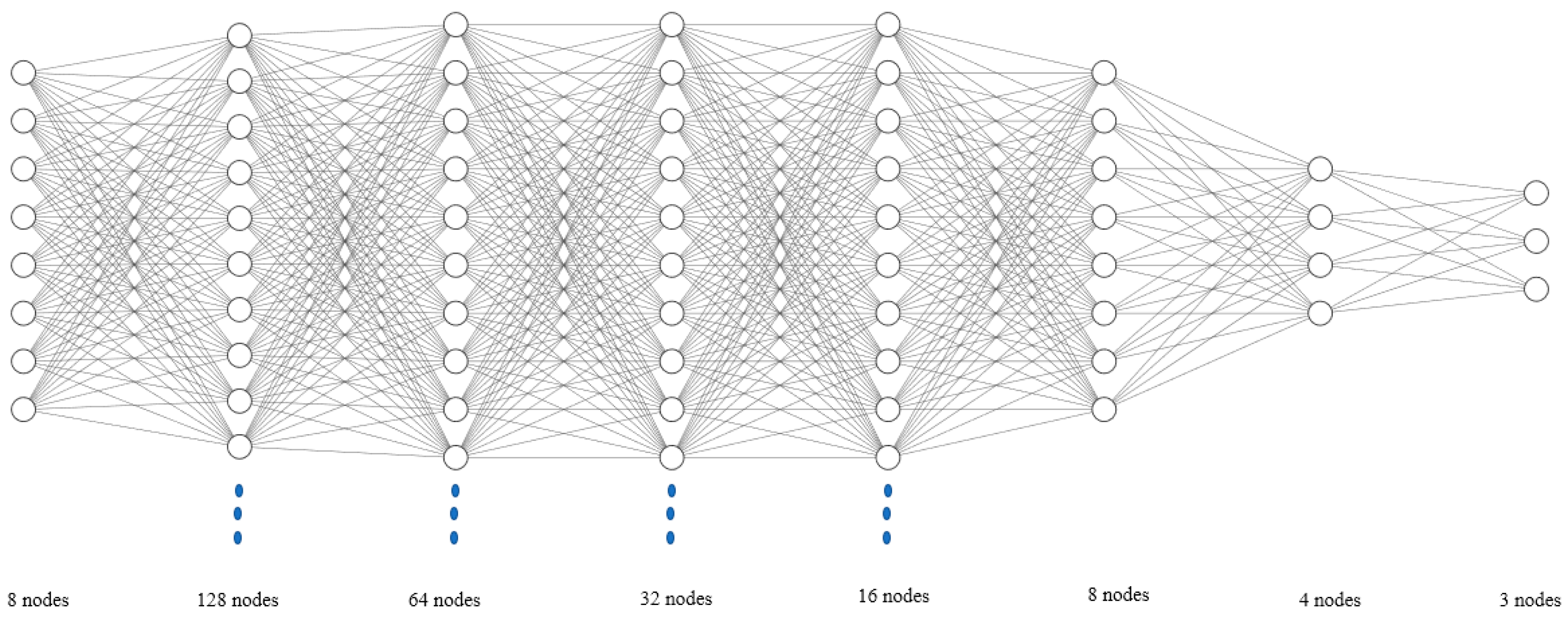
Artificial neural networks (ANNs) are mathematical mapping tools inspired by the human brain. The present study involves developing an ANN-based surrogate model. ANNs are made up of layers, as seen in Figure 2: an input layer, hidden layers, and an output layer. These layers consist of interconnected neurons. Each neuron has an associated weight and threshold. An individual neuron is activated if its output is above the specified threshold value; this sends data to the next layer. Otherwise, the data are not passed along to the next network layer. Different activation functions are used at each layer.
Individual neurons are similar to regression models, with input data, weights, a bias (or threshold), and an output. An example formula at the neuron level is shown below:
a: sum of weighted average; b: bias; w: weight; i: index.
An individual neuron computes the weighted averages of its input, and the sum is passed to an activation function which produces an output to pass along to the next layer. The output of one neuron becomes the input of the next neuron. Common activation functions include sigmoid, the exponential linear unit, the rectified exponential linear unit (ReLU), and many others. The output from each neuron can be found as:
where g is the activation function. The process of passing data from one layer to the next is what makes it a feedforward ANN.
The ANN calculates the input and output equations for each layer. Training a model involves evaluating its accuracy, which is performed by defining a cost (or loss) function. In most regression problems, the cost function is the mean squared error (MSE). The MSE can be found as:
i: sample index; : predicted outcome; y: actual value; m: total samples.
Finally, the weights and biases are updated through an iterative process to minimize the MSE and obtain an accurate model accordingly.
Figure 2 shows the schematic of the network structure that is used in this study. Six layers were used as they provided the best convergence. Additionally, two dropout layers at a rate of 0.2 were used to prevent overfitting.
A Python script was developed to automate the supply of 200 series of input data to EnergyPlus and to collect the simulation results accordingly. Eight parameters were selected and were varied within the specified ranges, as shown in Table 2.
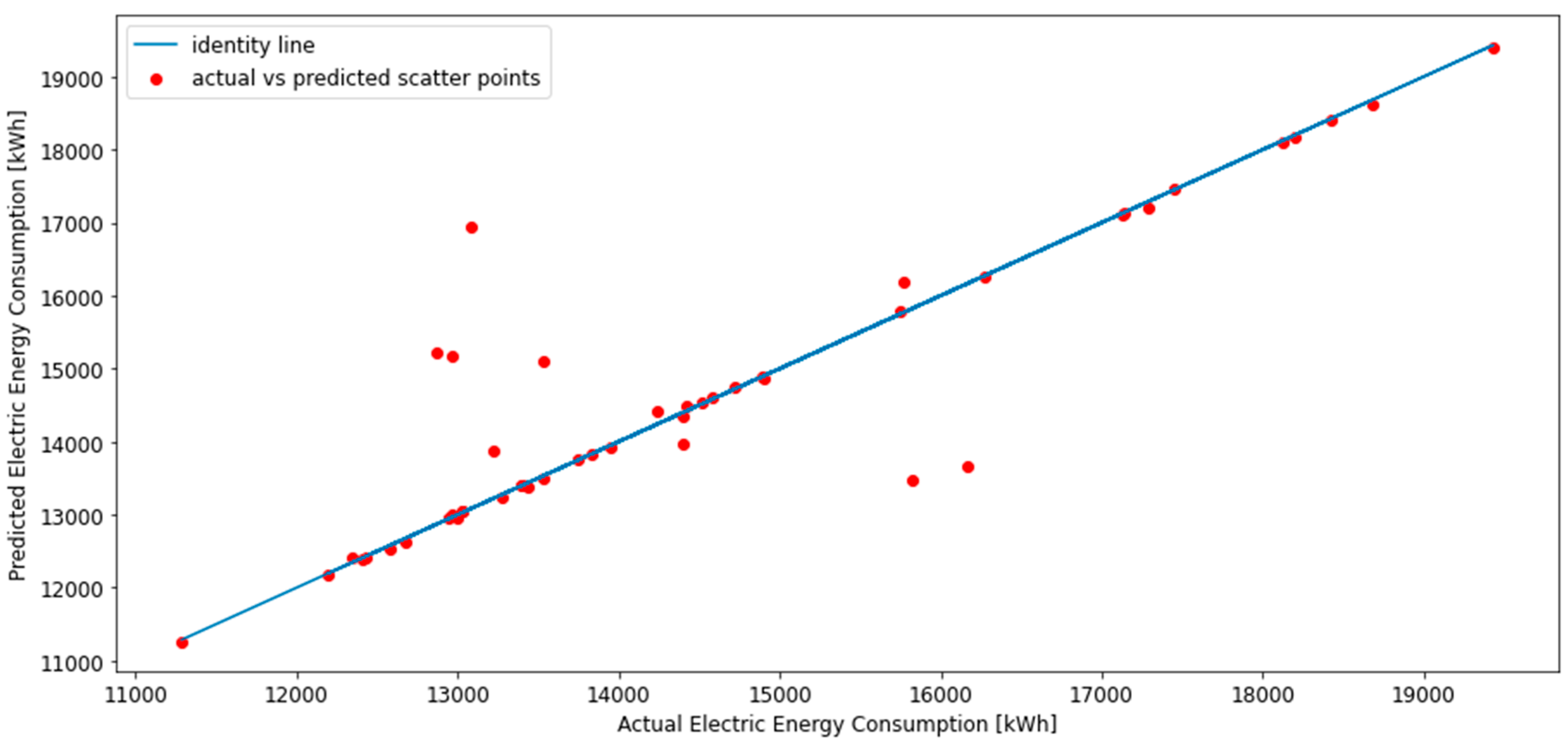
The generated data representing the design parameters and their respective annual energy consumption values were divided into a training dataset (80%) and a training and validation dataset (20%). Different design models were generated for the ANN training and testing using a Python automation script to generate 200 distinct models. An API was used to access EnergyPlus on a local machine and given several design inputs to simulate a new BEM; this is described further in Section 4. Five-fold cross-validation was used in this section to validate the performance of this model. The K-fold cross-validation did not show a significant difference from the initial model. The minimum loss values for the training and testing sets were found to have an RMSE of 0.075 for training and 1.153 for testing. The model performance is depicted in the correlation graph shown in Figure 3.
An R2 coefficient of determination was also used as a metric to measure the accuracy of the surrogate for the newly introduced data; the surrogate model achieved a maximum of 90% R2 by performing hyperparameter tuning. This is achieved by using random search and developing a hyperparameter search space for alpha for regularization strength, fit intercept, the solver to use in computational routines, and the normalization implementation. Model epochs and optimizer learning rates were also evaluated to find a model that performed well.
3. Building Energy Model Optimization
3.1. Optimization Approaches
The optimization variables used in this study are listed in Table 3. Two optimization approaches are used in this study to demonstrate how the developed framework allows the performance of optimization using available open-source programming tools such as Python and to show that it is highly achievable. The two approaches that are presented here include the genetic algorithm and the Bayesian algorithm, which are discussed in Section 3.1.1 and Section 3.1.2, respectively. Other optimization tools, such as particle swarm optimization, ant colony optimization, differential evolution, and the stochastic algorithm can also be implemented within a Python programming environment. The minimization function approach taken in this study is presented in Equation 4, as shown below.
Equation (4) constrained to Table 1.
3.1.1. Genetic Algorithm Framework
A genetic algorithm is an optimization algorithm, inspired by natural evolution, which can be used for the global minimization of objective functions [25]. The genetic algorithm has proved to be very effective for solving various engineering problems involving constrained, multi-variable optimizations with non-linear objective functions [26].
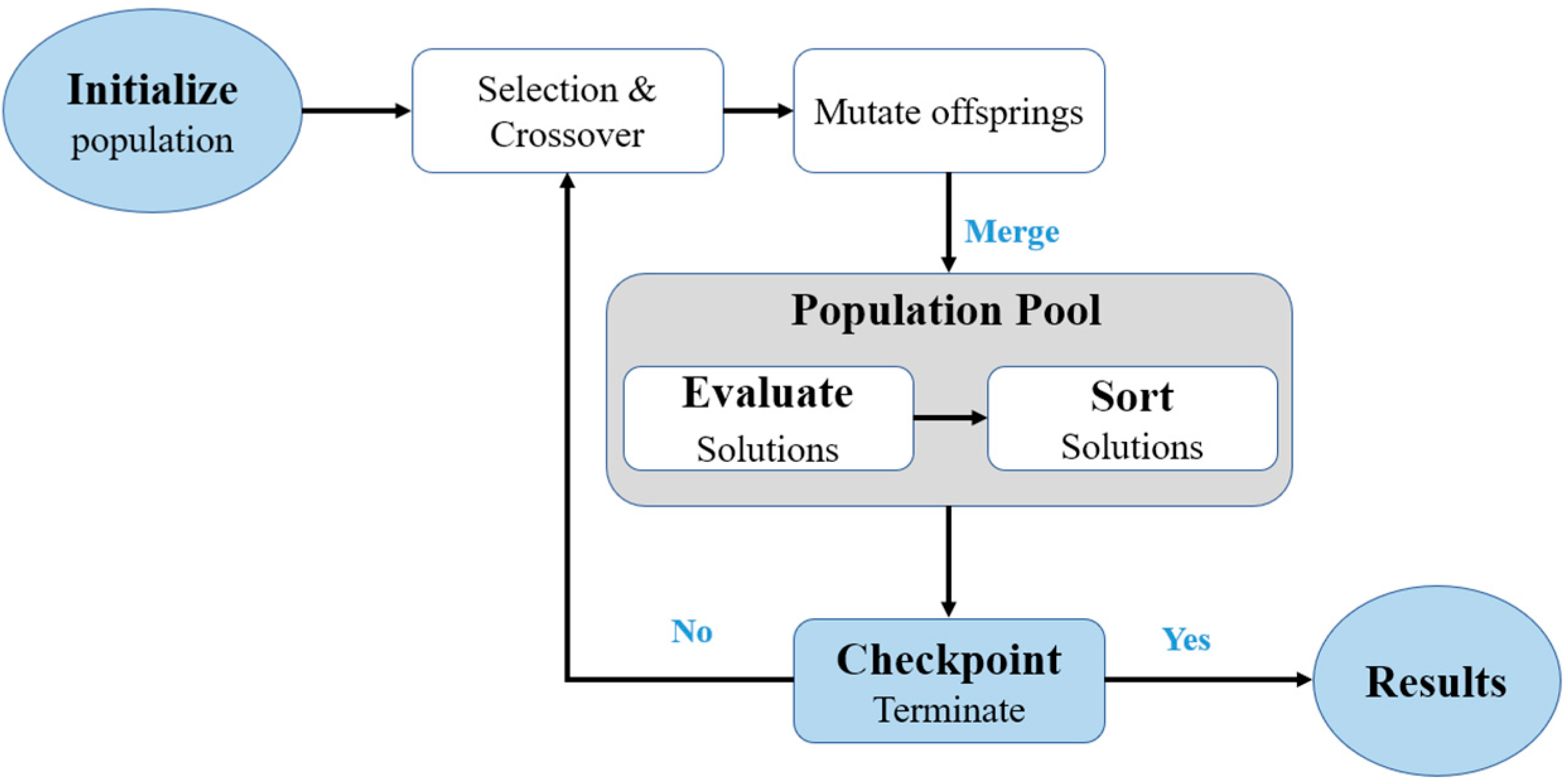
Genetic optimization lies in the classification of algorithms known as evolutionary algorithms (EAs). Unlike traditional algorithm methods, the EAs are not static but dynamic, which means that they evolve. The evolutional optimization approach is appropriate for this study, given the relatively large number of variables and the non-linear nature of the objective function (i.e., annual building energy consumption). The flow chart shown in Figure 4 summarizes the steps through which the genetic algorithm is being implemented. It begins by initializing a population: the first generation, from randomly chosen individuals (i.e., random combinations of optimization variables). Members are selected from the first generation. These members depict chromosomes containing a certain number of genes (optimization variables). A new generation is created by reproduction, which involves a crossover (mating) from the member solutions. A random change, like a gene mutation, is involved in creating a new generation. The process continues until a termination criterion is met: either enough best solutions are found or a defined maximum number of generations is reached.
The optimization process was carried out in five steps. The first step was population initialization, which was achieved by producing 50 different outputs from the surrogate model and saving the corresponding values for each design variable.
The second step is candidate selection. The selection process involves taking candidates from the population in the mating pool. Based on the previously calculated energy consumption value, a threshold (a lower energy consumption than previously calculated) is used to select the best individuals. From the selected subset, the parents are prepared for mating. Selecting the parents to be used in mating is performed using the roulette wheel selection, which is an efficient way of selecting candidates by giving a higher probability of selection to the parents that have a lower energy consumption design model. The third step involves crossover, where the offspring are generated from two candidate parents, a parameter that is tuned with a probability value. These offspring have similar genetic properties to their parents, mathematically represented as decimal values in this study. The offspring are then mutated (the probability value is used for tuning) to provide a different version with different genetic properties to its parent. New offspring are merged with the population, and the pool is sorted. Poor candidates are eliminated from the population. The remaining population is part of a new generation that undergoes a similar process starting from step 1 until a solution with the lowest energy consumption cannot be overtaken. The process should be conducted in only 100 iterations; thus, either the minimum or the energy consumption is reached, or the maximum iterations are reached. The last step is terminating the process when the best solution is reached. All the optimization parameters used for the genetic algorithm are listed in Table 4.
The GA optimization approach minimizes the energy consumption of the surrogate model. In other words, the GA determines the design variables that produce a building model with minimized energy use. The surrogate model is used as a fitness function to find a building design that may provide a lower energy consumption. These results can be compared to the results and the design obtained when the minimization is completed by using the Bayesian algorithm.
3.1.2. Bayesian Algorithm
The Bayesian optimization algorithm stems from the Bayes theorem of conditional probability calculated when the joint probability is challenging to calculate or when a reverse conditional probability is available. The concept is applied in optimization as a way of finding the extrema of an objective function that is expensive to evaluate. As the Bayes theorem can provide an approximation of the objective function, it can be used to estimate the cost of the different variables that we wish to evaluate. A Bayesian algorithm, therefore, creates a surrogate objective function of the problem in question, which can then be optimized. The Bayesian algorithm uses an acquisition function to search for probable candidates to be evaluated. The Gaussian process is Bayesian in nature, being a probability distribution over all possible functions. Nonetheless, Bayesian approaches use the surrogate optimization method. In short, the GA is a population-based optimization method; the Bayesian approach can optimize functions by building a statistical model—in other words, it is an estimation of the distribution algorithm. Therefore, it is important to evaluate the Bayesian performance as an alternative optimization tool when it comes to ANN-based building energy surrogate models. The parameters used for this algorithm are listed in Table 5.
An available package within Python called Scikit Optimizer allows the implementation of the Bayesian optimization on the surrogate model. A simple Bayesian optimization algorithm pseudocode used in this study is presented in Algorithm 1:
| Algorithm 1: Basic pseudocode for the Bayesian optimization algorithm |
| def optimize(f, bounds, num_iterations): # Initialize the algorithm with a set of observations observations = initialize(bounds) for i in range(num_iterations): # Fit a probabilistic model to the observations model = fit_model(observations) # Select the next input values to evaluate based on the model x = select_inputs(model, bounds) # Evaluate the function at the selected input values y = f(x) # Add the new observations to the set of observations observations.append((x, y)) |
4. Python Platform
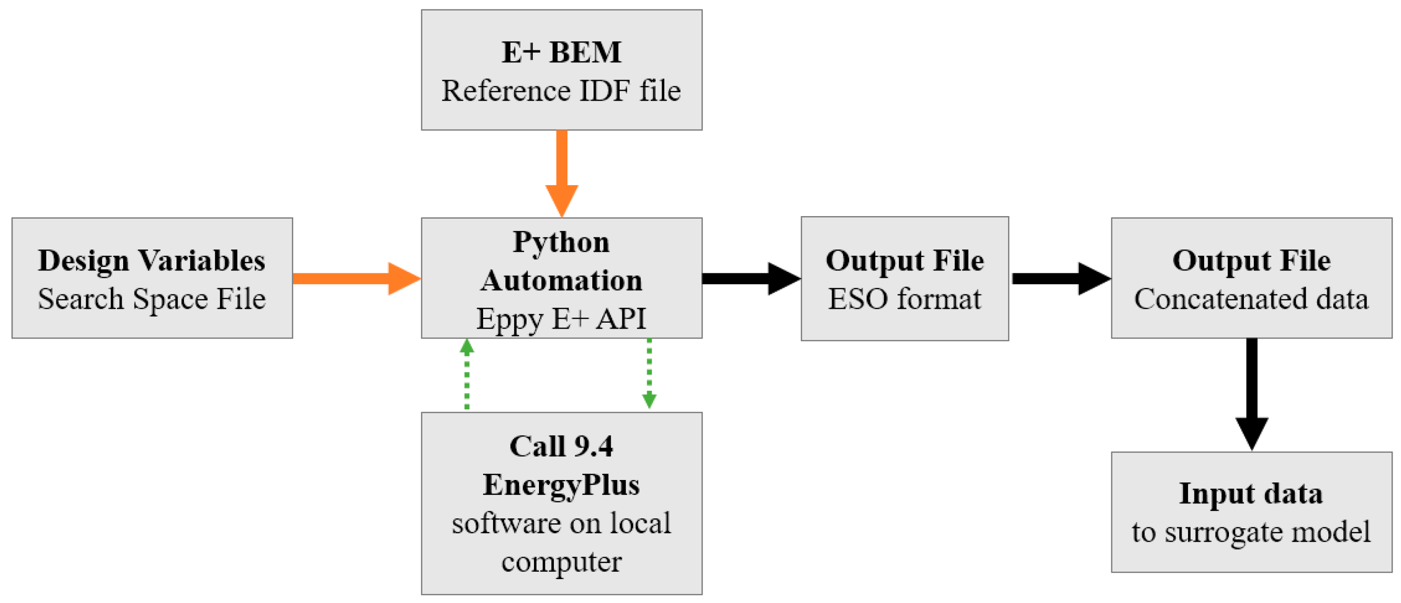
In this study, a Python script is developed to facilitate the data entry and perform simulations on locally installed EnergyPlus software iteratively. Running multiple simulations is automated to reduce the time that would otherwise be taken to manually run individual simulations and later gather all the data needed to develop the ANN surrogate model. A Python package, Eppy [27], was used to work with EnergyPlus using Python. The flow chart of steps that are followed for establishing the surrogate model using Python is presented in Figure 5. The baseline model IDF file containing all the design variables and components of the building energy model is imported into the Python program. The IDF file and the variable search space file are inputs into the Eppy API that runs the EnergyPlus on a local computer. Table 1 shows all eight design and control parameters changed at each simulation run to generate subsequent energy consumption, production, and net site energy. A total of 200 changes are performed for each design parameter, and the values are randomly selected between the ranges provided in Table 2 for each variable. There are 200 rows and 11 columns containing the design variable values and simulation results, represented as annual electricity consumption, production, and net site energy. Each row of data has its specific IDF file containing the design variables of that row. This IDF can be simulated in EnergyPlus to produce the desired output; only three annual results are used for this study.
At this stage, the Python package has helped create a dataset that can be used for the ANN model development. Suppose a random user wants to perform a test using the Python auto-simulation program developed here. In that case, they need a reference IDF file that they want to study and specified ranges of the design variables they desire to change within the IDF. Thus, the auto-simulation program can quickly generate a dataset for the ANN model development, as is the case for this study, or other parametric analysis tools desired by the user. The auto-simulation program makes data generation easier and computationally cheap.
The genetic algorithm is also developed and implemented using Python. The objective function is created by making a function that accepts an array containing values for the seven variables listed in Table 1. The function then returns the predicted energy consumption of a building model with the provided variable inputs. The prediction is performed by the surrogate model. Furthermore, the function parameters, including population size, mutation rate, and number of iterations and generations, are defined and used to tune the GA model. A separate library is developed to:
- Initialize the population;
- Select parents using a roulette wheel selection approach;
- Perform crossover and mutation;
- Evaluate offspring (then merge, sort, and select again);
- Determine and store the chromosomes with the lowest values of the cost function in each iteration;
- Define the selection process for selecting a new population once merging and sorting have been implemented on the current population.
Similarly, the Bayesian method is implemented after defining the objective function (i.e., the annual energy consumption). The Scikit-Optimize package is imported into the Python environment, and the Bayesian optimization solution based on the Gaussian process regression [28] is implemented.
5. Results and Discussions
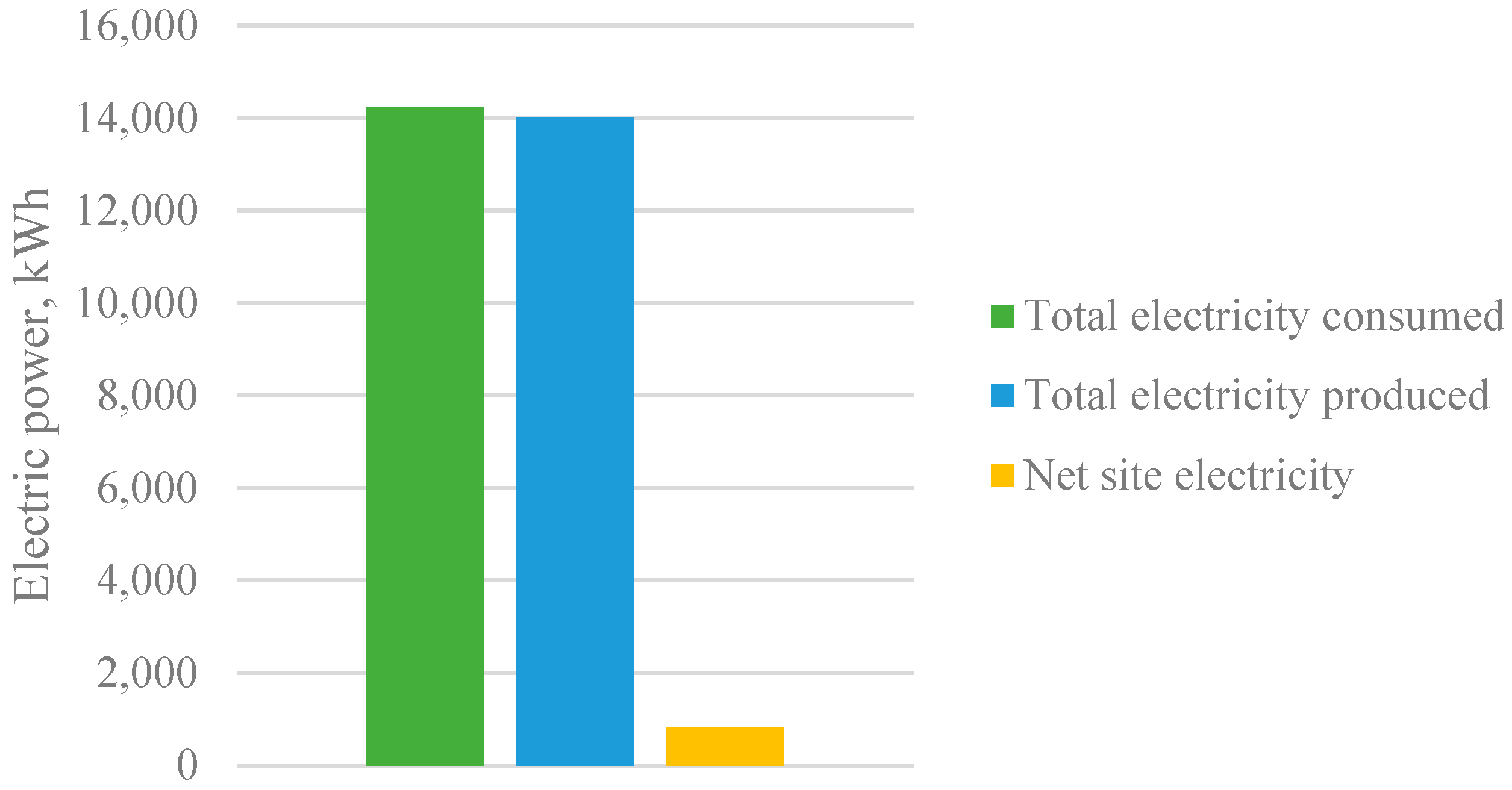
After performing the simulation and crosschecking with the initial design simulations to confirm the degree of accuracy, the surrogate model was ready to be used for optimization. The surrogate model simulation results for the same design inputs to the baseline model agreed with the simulations obtained from the EnergyPlus modeling software. Figure 6 demonstrates the predicted energy use from the EnergyPlus simulation, which is used as a benchmark for optimization. This information is also summarized in Table 6.
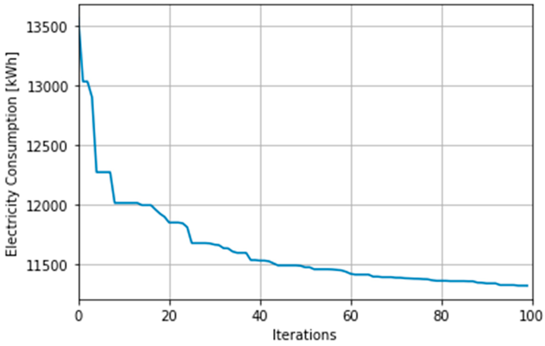
The surrogate model was used as a fitness function for the genetic optimization and compared with those obtained with the Bayesian optimization. The objective functions are optimized with respect to the seven design and control variables in Table 2 (first seven rows), which are constrained to their respective intervals. Figure 7 presents the minimization trend followed by the GA for 100 iterations. The computation started converging after 40 epochs, and the total computation time was 5 min and 36 s for a maximum of 100 iterations and an initial population size of 50. It should be noted that using a larger population size would result in a longer computation time.
The GA minimizes the energy consumption of the baseline model from 14 MWh per year to 11.3 MWh per year, which is a significant improvement in terms of energy consumption. The lower energy consumption is mainly achieved by the GA choosing a design model with more efficient design variables (as listed in Table 7).
The design variables in this model practically provide better energy efficiency. The cooling setpoint is in the range that would provide a lower energy consumption by the HVAC system. The window U-value decision is considerably higher than the U-values for the windows used in the building construction. This could result from the surrogate model errors resulting from a lack of proper window U-values and energy consumption correlation.
The recommended designs were then implemented in the EnergyPlus software to compare with the results from the surrogate model optimization. The EnergyPlus simulation results show a reduced energy consumption, down to 12,420 kWh. Thus, there is a 9.9% percent error between the optimization results using the ANN-based surrogate model and the EnergyPlus model.
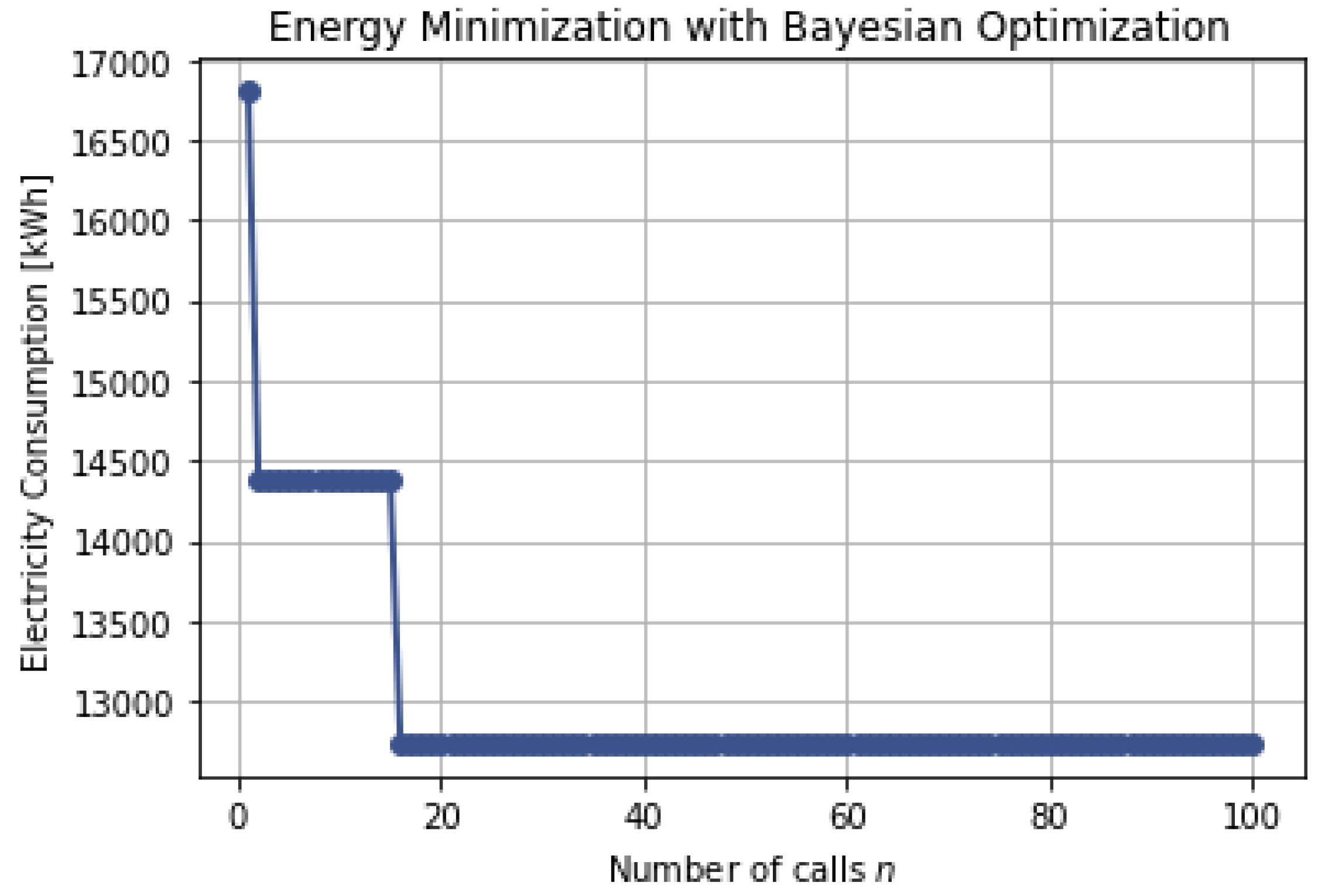
Likewise, the Bayesian optimization results are shown in Figure 8, and the tabulated results are presented in Table 8 for 100 iterations. As expected, the Bayesian optimization takes a shorter computational time compared with the genetic optimization.
The Bayesian optimization converges after 20 iterations and takes a shorter computational time. The total time for all 100 iterations was 59.5 s, which was still a faster computational time than the time taken by the GA optimization. The Bayesian optimization can minimize building design energy consumption from 14 MWh to 12.7 MWh. The optimal design variables that are obtained using Bayesian optimization are listed in Table 8. This is a minimization that is not as low as the one achieved by the GA, but it does provide lower consumption than the EnergyPlus baseline model’s energy consumption estimates.
The Bayesian optimization results show an approach to lower energy consumption by increasing the wall R-value and the cool setpoint. However, the roof R-values and window U-values can be increased to have an even lower energy consumption.
The optimization process in this study creates a benchmark for a more complex optimization approach that involves the use of other variables such as variable electricity rates, systems life cycle costs, etc. Additionally, the surrogate model could be improved in a way that provides the GA with multi-objective fit functions to optimize several variables at the same time. Such additional variables could be electricity cost and visual and thermal comfort.
The recommended designs by Bayesian optimization are then implemented in the EnergyPlus software to compare with the results from the surrogate model optimization. The EnergyPlus simulation results show a reduced energy consumption down to 13,613 kWh. Thus, there is a 6.86% percent error between the Bayesian optimization results on the surrogate model and the EnergyPlus model. These errors are not attributed to the optimization algorithms as they are associated with the ANN-based surrogate model and do not provide any basis of comparison for the optimization algorithms.
6. Discussion
The surrogate modeling proved to be more computationally efficient in estimating building energy consumption when compared to the physics-based BEM software tools such as EnergyPlus, at the expense of an extensive training process to have a well-generalized ANN-based surrogate model. The surrogate model must be tested and modified multiple times before an accurate predictive model is achieved.
Energy optimization with a genetic algorithm uses the surrogate model as a fitness function with seven variables. These variables have a defined design search space to perform a function minimization that produces the least annual energy-consuming design model. Other methods can be used for optimizing the surrogate models. However, the genetic algorithm was chosen for its evolutionary approach to solving a given problem that tends to go a step further in finding the best solutions, unlike the traditional optimization methods such as the gradient descent methods. Nonetheless, the GA optimization performance is compared with an easy-to-implement Bayesian optimization available in a Python package in order to be easily integrated with the developed surrogate model. As expected, the GA optimization provided designs that can achieve a lower annual building energy consumption. Similarly, Bayesian optimization also produces designs with lower building energy consumption than the baseline model while requiring less computation time. The GA optimization was able to provide lower energy-efficient solutions than the Bayesian optimization. The GA optimization made a balanced improvement to all the design variables to obtain the best solution, unlike the Bayesian optimization which seemed to stick to those design variables (such as the wall R-value and the cooling setpoints) that provide the best solution and to keep making them better.
7. Conclusions
In this study, a novel approach is presented for applying advanced optimization techniques to building energy models using Python EnergyPlus. The data entry process to EnergyPlus is facilitated through a Python script and 200 possible designs that cover the desired ranges of eight variables that are simulated for a case study building. The resulting datasets are then used to train an ANN which serves as a surrogate BEM. Two different optimization techniques, including Bayesian optimization and a genetic algorithm, are then applied to the surrogate BEM, and the results are discussed in detail. The ANN model achieved a maximum of 90% R2 through hyperparameter tuning. The optimal designs that were obtained by applying the genetic algorithm and Bayesian optimization led to annual building energy consumptions of 11.3 MWh and 12.7 MWh, respectively. It was shown that the approach that was presented bridges the gap between the physics-based building energy models and the strong optimization tools available in Python, which can allow the achievement of the global optimization in a computationally efficient fashion. The approach presented in this study can be implemented for various types of buildings with different applications and design parameters to achieve optimal building energy performance.
Author Contributions
Conceptualization, B.K. and H.N.; methodology, H.N.; software, B.K.; validation, H.N.; formal analysis, B.K. and H.N.; investigation, B.K.; resources, B.K. and H.N.; data curation, B.K.; writing—original draft preparation, B.K.; writing—review and editing, H.N.; visualization, B.K.; supervision, H.N.; project administration, H.N. All authors have read and agreed to the published version of the manuscript.
Funding
This research was funded in part by the IRI grant from the College of Engineering and Science of Florida Institute of Technology.
Informed Consent Statement
Not applicable.
Data Availability Statement
All models and sample data are available on GitHub https://github.com/bkubwimana2016/Neural-Networks-for-BEM.
Conflicts of Interest
The authors declare no conflict of interest.
References
- Baldwin, S. Quadrennial Technology Review: An Assessment of Energy Technologies and Research Opportunities; U.S. Department of Energy: Washington, DC, USA, 2015. [Google Scholar]
- Chantrelle, F.P.; Lahmidi, H.; Keilholz, W.; El Mankibi, M.; Michel, P. Development of a multicriteria tool for optimizing the renovation of buildings. Appl. Energy 2011, 88, 1386–1394. [Google Scholar] [CrossRef]
- Kurniawan, B.; Song, W.; Weng, W.; Fujimura, S. Distributed-elite local search based on a genetic algorithm for bi-objective jobshop scheduling under time-of-use tariffs. Evol. Intell. 2020, 14, 1581–1595. [Google Scholar] [CrossRef]
- Ene, S.; Küçükoğlu, İ.; Aksoy, A.; Öztürk, N. A genetic algorithm for minimizing energy consumption in ware-houses. Energy 2016, 114, 973–980. [Google Scholar] [CrossRef]
- Santos, R.S.; João, M.; Abreu, A. Getting efficient choices in buildings by using Genetic Algorithms: Assessment & validation. Open Eng. 2019, 9, 229–245. [Google Scholar]
- Karaguzel, O.T.; Zhang, R.; Lam, K.P. Coupling of whole-building energy simulation and multi-dimensional numerical optimization for minimizing the life cycle costs of office buildings. Build. Simul. 2013, 7, 111–121. [Google Scholar] [CrossRef]
- Rabani, M.; Madessa, H.B.; Nord, N. Achieving Zero-Energy Building Performance with Thermal and Visual Comfort Enhancement through Optimization of Fenestration, Envelope, Shading Device, and Energy Supply System. Sustain. Energy Technol. Assess. 2021, 44, 101020. [Google Scholar] [CrossRef]
- Corbin, C.D.; Henze, G.P.; May-Ostendorp, P. A model predictive control optimization environment for real-time commercial building application. J. Build. Perform. Simul. 2013, 6, 159–174. [Google Scholar] [CrossRef]
- Migliori, M.; Najafi, H.; Fabregas, A.; Nguyen, T. Neural Network-Based Building Energy Models for Adapting to Post-Occupancy Conditions: A Case Study for Florida. ASME J. Eng. Sustain. Build. Cities 2022, 3, 041002. [Google Scholar] [CrossRef]
- Li, K.; Pan, L.; Xue, W.; Jiang, H.; Mao, H. Multi-Objective Optimization for Energy Performance Improvement of Residential Buildings: A Comparative Study. Energies 2017, 10, 245. [Google Scholar] [CrossRef] [Green Version]
- Magnier, L.; Haghighat, F. Multiobjective optimization of building design using TRNSYS simulations, genetic algorithm, and Artificial Neural Network. Build. Environ. 2010, 45, 739–746. [Google Scholar] [CrossRef]
- Jain, A.; Smarra, F.; Reticcioli, E.; D’Innocenzo, A.; Morari, M. NeurOpt: Neural network based optimization for building energy management and climate control. In Proceedings of the 2nd Annual Conference on Learning for Dynamics and Control, Proceedings of Machine Learning Research, Berkeley, CA, USA, 11–12 June 2020; 120, pp. 445–454. [Google Scholar]
- Jiang, Z.; Risbeck, M.J.; Ramamurti, V.; Murugesan, S.; Amores, J.; Zhang, C.; Lee, Y.M.; Drees, K.H. Building HVAC control with reinforcement learning for reduction of energy cost and demand charge. Energy Build. 2021, 239, 110833. [Google Scholar] [CrossRef]
- Li, Y.; Nord, N.; Zhang, N.; Zhou, C. An ANN-based optimization approach of building energy systems: Case study of swimming pool. J. Clean. Prod. 2020, 277, 124029. [Google Scholar] [CrossRef]
- Li, H.; Liang, X.; Xu, J. Building Energy Optimization Based on Biased ReLU Neural Network. In Proceedings of the 2021 40th Chinese Control Conference (CCC), Shanghai, China, 26–28 July 2021. [Google Scholar] [CrossRef]
- Gossard, D.; Lartigue, B.; Thellier, F. Multi-objective optimization of a building envelope for thermal performance using genetic algorithms and artificial neural network. Energy Build. 2013, 67, 253–260. [Google Scholar] [CrossRef] [Green Version]
- Asadi, E.; da Silva, M.G.; Antunes, C.H.; Dias, L. Multi-objective optimization for building retrofit strategies: A model and an application. Energy Build. 2012, 44, 81–87. [Google Scholar] [CrossRef]
- Bamdad, K.; Cholette, M.E.; Bell, J. Building energy optimization using surrogate model and active sampling. J. Build. Perform. Simul. 2020, 13, 760–776. [Google Scholar] [CrossRef]
- Doiphode, G.; Najafi, H. A Machine Learning Based Approach for Energy Consumption Forecasting in K-12 Schools. In Proceedings of the ASME 2020 International Mechanical Engineering Congress and Exposition, Virtual, 16–19 November 2020; Volume 8, p. V008T08A032. [Google Scholar] [CrossRef]
- Lara, R.A.; Naboni, E.; Pernigotto, G.; Cappelletti, F.; Zhang, Y.; Barzon, F.; Gasparella, A.; Romagnoni, P. Optimization Tools for Building Energy Model Calibration. Energy Procedia 2017, 111, 1060–1069. [Google Scholar] [CrossRef]
- Aijazi, A.N.; Glicksman, L.R. Application of surrogate modeling to multi-objective optimization for residential retrofit design. In Proceedings of the Symposium on Simulation for Architecture and Urban Design (SIMAUD ‘19); Society for Computer Simulation International: San Diego, CA, USA, 2019; pp. 1–7. [Google Scholar]
- Aydın, E.E.; Dursun, O.; Chatzikonstantinou, I.; Ekici, B. Optimisation of Energy Consumption and Daylighting using Building Performance Surrogate Model. In Proceedings of the Architectural Science Association Conference, Melbourne, Australia, 2–4 December 2015. [Google Scholar]
- Amoah, K.; Nguyen, T.; Najafi, H. A Multi-Facet Retrofit Approach to Improve Energy Efficiency of Existing Class of Single-Family Residential Buildings in Hot-Humid Climate Zones. Energies 2020, 13, 1178. [Google Scholar]
- Betharte, O.; Najafi, H.; Nguyen, T. Towards Net-Zero Energy Buildings: A Case Study in Humid Subtropical Climate. In ASME International Mechanical Engineering Congress and Exposition; American Society of Mechanical Engineers: Pittsburgh, PA, USA, 2018. [Google Scholar]
- Najafi, H.; Najafi, B. Multi-objective optimization of a plate and frame heat exchanger via genetic algorithm. Heat Mass Transf. 2010, 46, 639–647. [Google Scholar] [CrossRef]
- Yang, P.; Najafi, H. A Comparative Study of Multi-Stage Approaches for Wind Farm Layout Optimization. J. Energy Resour. Technol. 2022, 144, 101302. [Google Scholar] [CrossRef]
- Philip, S. EPPY (2021), EPPY 0.5.56—EnergyPlus Python. Available online: https://pypi.org/project/eppy/ (accessed on 1 July 2021).
- Head, T.; Kumar, M.; Nahrstaedt, H.; Louppe, G.; Shcherbatyi, I. Scikit-Optimize/scikit-Optimize (v0.9.0). Zenodo. Available online: https://zenodo.org/record/5565057#.Y8Y-iRVBxPY (accessed on 1 July 2021).
Figure 1.
Florida Tech Alumni Center (building used for the case study).

Figure 2.
Schematic of ANN architecture.

Figure 3.
Correlation between EnergyPlus (true values) and surrogate model-predicted energy consumption.
Figure 3.
Correlation between EnergyPlus (true values) and surrogate model-predicted energy consumption.

Figure 4.
Genetic algorithm flowchart.

Figure 5.
Steps toward building a surrogate model.

Figure 6.
Annual energy use (case study building).

Figure 7.
Minimizing building’s energy consumption (surrogate model) using genetic algorithm.

Figure 8.
Minimizing building’s energy consumption (surrogate model) using Bayesian optimization.


Table 1.
Parameters used for the baseline model.
| Parameter | Parameter Values | Units |
|---|---|---|
| Wall R-value | 10.1 | m2K/W |
| Roof R-value | 31.49 | m2K/W |
| HVAC Cooling COP 47C, 3 units | 3.9, 4.4, 3.7 | - |
| Window U-value | 1.22 | W/m2K |
| Window SHGC | 0.40 | - |
| Cool Setpoint | 23.4 | °C |
| Light power density | 7.5 | W/m2 |
| PV Tilt Angle | 20 | ° |
| Lowest Annual Energy Consumption | 14,243 | kWh |
Table 2.
Respective ranges for the variables used in developing ANN training data.
| Parameter | Minimum | Maximum | Unit |
|---|---|---|---|
| Wall R-value | 8 | 25 | m2K/W |
| Roof R-value | 25 | 45 | m2K/W |
| Window U-value | 1 | 7 | W/m2K |
| Window SHGC | 0.2 | 0.7 | - |
| Cooling Setpoint | 21 | 26 | °C |
| HVAC Cooling COP | 2 | 5.5 | - |
| Light Power Density | 2 | 15 | W/m2 |
| PV Tilt Angle | 10 | 35 |
Table 3.
Optimization variables and ranges.
| Variable | Minimum | Maximum |
|---|---|---|
| X1 = Wall R-value | 8 | 25 |
| X2 = Roof R-value | 25 | 45 |
| X3 = Window U-value | 1 | 7 |
| X4 = Window SHGC | 0.2 | 0.7 |
| X5 = Cooling Setpoint | 21 | 26 |
| X6 = HVAC Cooling COP | 2 | 5.5 |
| X7 = Light power density | 2 | 15 |
Table 4.
Genetic algorithm optimization parameters.
| Variable | Value |
|---|---|
| Population size | 50 |
| Mutation rate | 0.01 |
| Mutation step size | 0.1 |
| Crossover Probability | 0.1 |
| Number of iterations | 100 |
| Number of variables | 7 |
| Percentage of children, PC | 1 |
| Beta, roulette wheel selection probability coefficient | 1 |
Table 5.
Bayesian optimization algorithm parameters.
| Probabilistic Model | Gaussian Process (GP) |
|---|---|
| Fit function: Acquisition function | EI(x) = max(0, μ(x) – f *) where:
|
| GP noise level | 0 |
| initial points | 7 |
Table 6.
Summarized annual energy use for the building.
| Variable | Minimum |
|---|---|
| Electricity Consumption | 14,243 kWh |
| Total Electricity Peak Demand | 10.15 kW |
| EUI (Energy use intensity) | 15 kBTU/ft2/year |
Table 7.
Optimal design variables obtained from GA optimization.
| Parameter | Best Solution | Units |
|---|---|---|
| Wall R-value | 24.4 | m2K/W |
| Roof R-value | 28.94 | m2K/W |
| HVAC Cooling COP | 4.33 | - |
| Window U-value | 4.75 | W/m2K |
| Window SHGC | 0.40 | - |
| Cool Setpoint | 25.6 | °C |
| Light power density | 2.01 | W/m2 |
| Lowest Annual Energy Consumption | 11,300.3 | kWh |
Table 8.
Optimal design variables obtained with Bayesian optimization.
| Parameter | Best Solution | Units |
|---|---|---|
| Wall R-value | 23 | m2K/W |
| Roof R-value | 27 | m2K/W |
| HVAC Cooling COP | 3.6 | - |
| Window U-value | 4 | W/m2K |
| Window SHGC | 0.44 | - |
| Cool Setpoint | 26 | °C |
| Light power density | 3 | W/m2 |
| Lowest Annual Energy Consumption | 12,738.2 | kWh |
Disclaimer/Publisher’s Note: The statements, opinions and data contained in all publications are solely those of the individual author(s) and contributor(s) and not of MDPI and/or the editor(s). MDPI and/or the editor(s) disclaim responsibility for any injury to people or property resulting from any ideas, methods, instructions or products referred to in the content. |
© 2023 by the authors. Licensee MDPI, Basel, Switzerland. This article is an open access article distributed under the terms and conditions of the Creative Commons Attribution (CC BY) license (https://creativecommons.org/licenses/by/4.0/).
Share and Cite
MDPI and ACS Style
Kubwimana, B.; Najafi, H. A Novel Approach for Optimizing Building Energy Models Using Machine Learning Algorithms. Energies 2023, 16, 1033. https://doi.org/10.3390/en16031033
AMA Style
Kubwimana B, Najafi H. A Novel Approach for Optimizing Building Energy Models Using Machine Learning Algorithms. Energies. 2023; 16(3):1033. https://doi.org/10.3390/en16031033
Chicago/Turabian StyleKubwimana, Benjamin, and Hamidreza Najafi. 2023. "A Novel Approach for Optimizing Building Energy Models Using Machine Learning Algorithms" Energies 16, no. 3: 1033. https://doi.org/10.3390/en16031033
Note that from the first issue of 2016, this journal uses article numbers instead of page numbers. See further details here.