
Offshore CO2 Capture and Utilization Using Floating Wind/PV Systems: Site Assessment and Efficiency Analysis in the Mediterranean


Abstract
:
1. Introduction
- Available power,
- Environmental risk,
- Available methanol production.
2. Materials and Methods
2.1. Power Generation
2.1.1. Solar
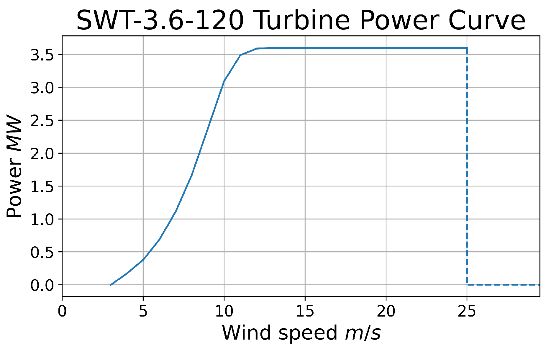
2.1.2. Wind
2.2. Environmental Risk
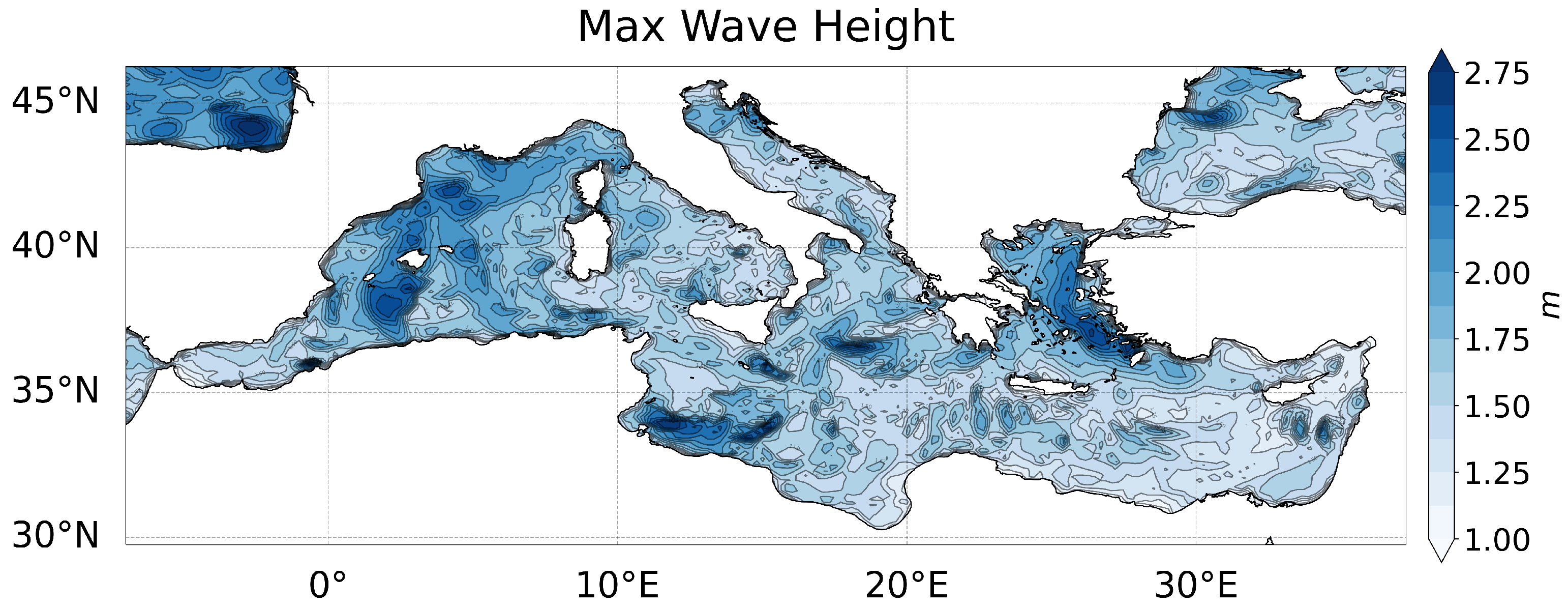
2.2.1. Max Wave Height
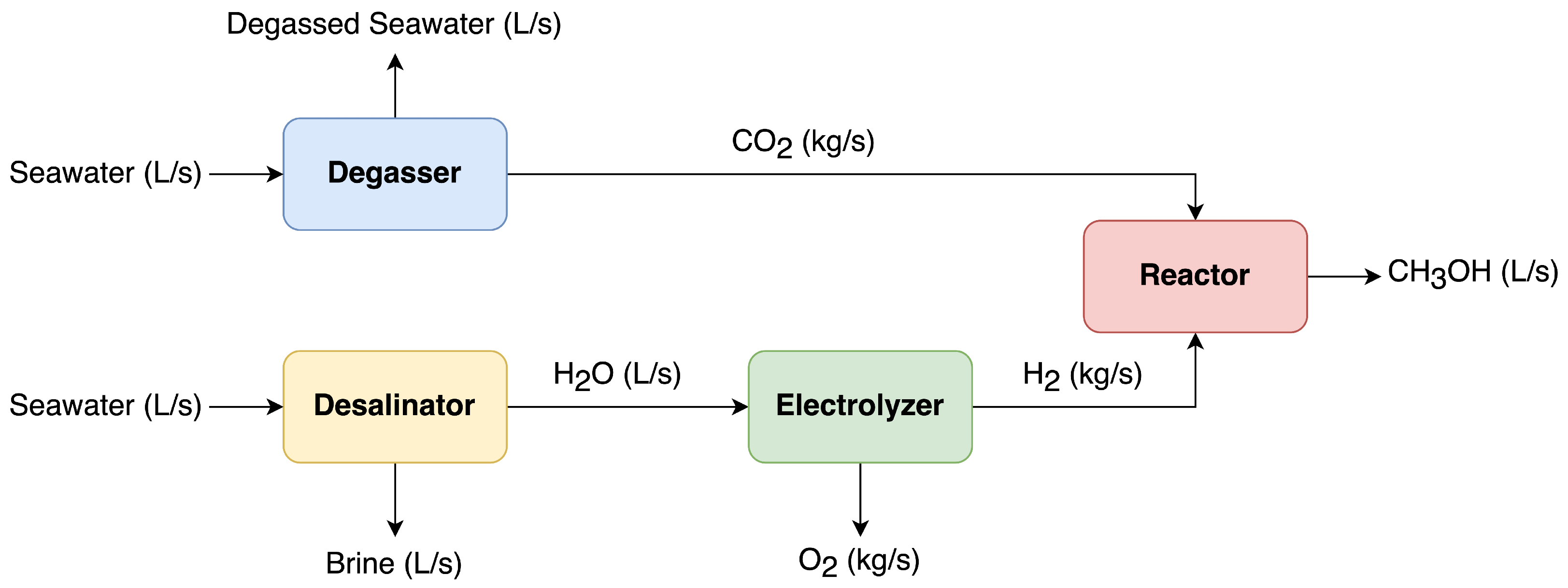
2.3. Methanol Production—pyseafuel
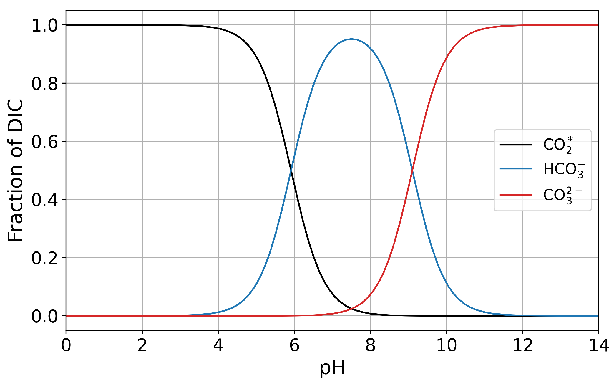
2.3.1. Degassing
2.3.2. Desalination
2.3.3. Electrolysis
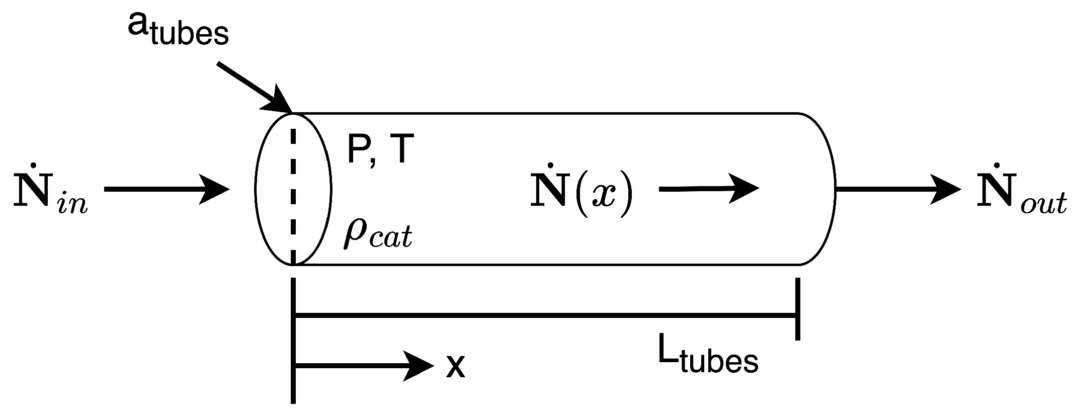
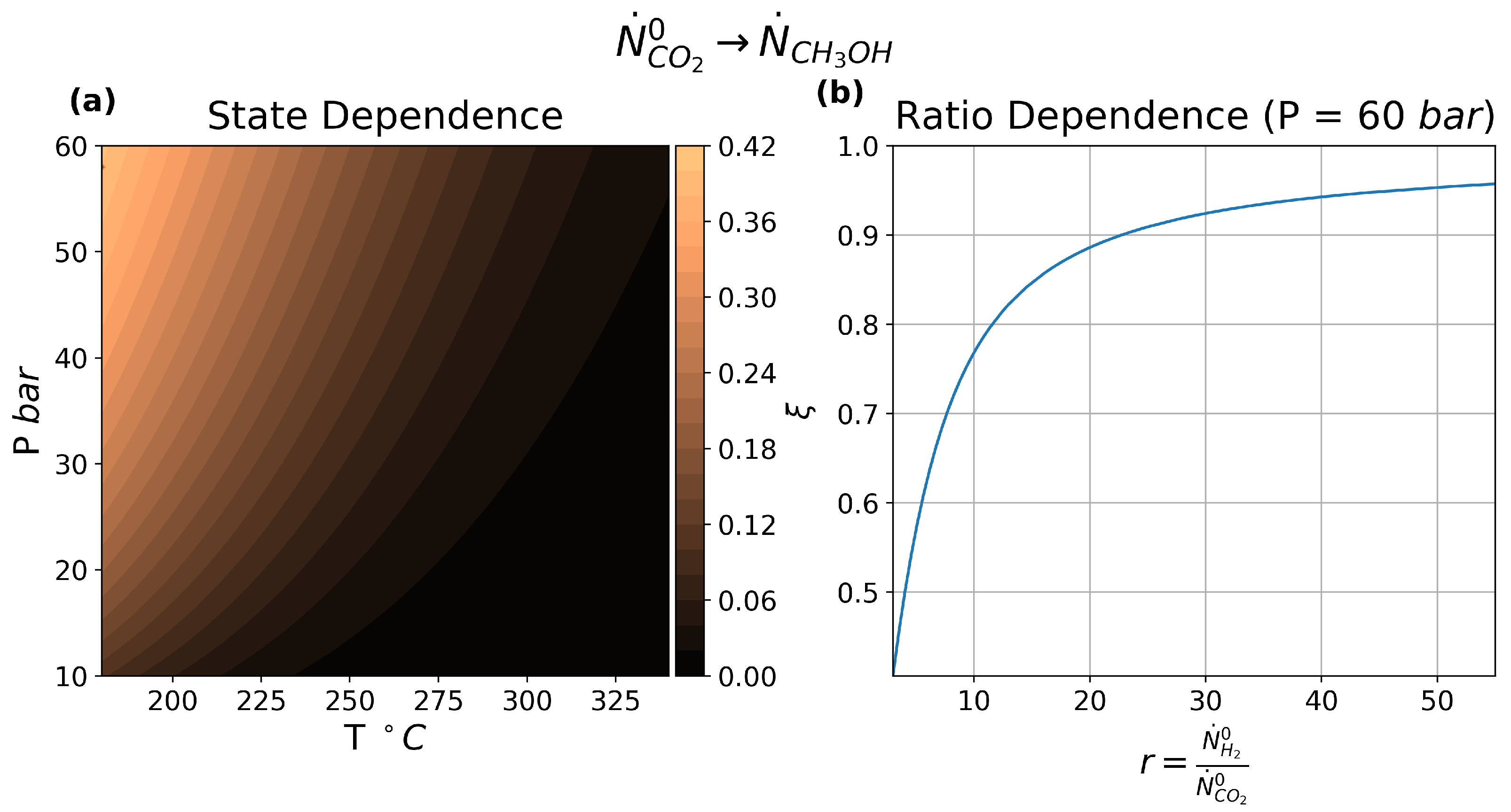
2.3.4. Reactor
3. Results and Discussion
3.1. Power Generation
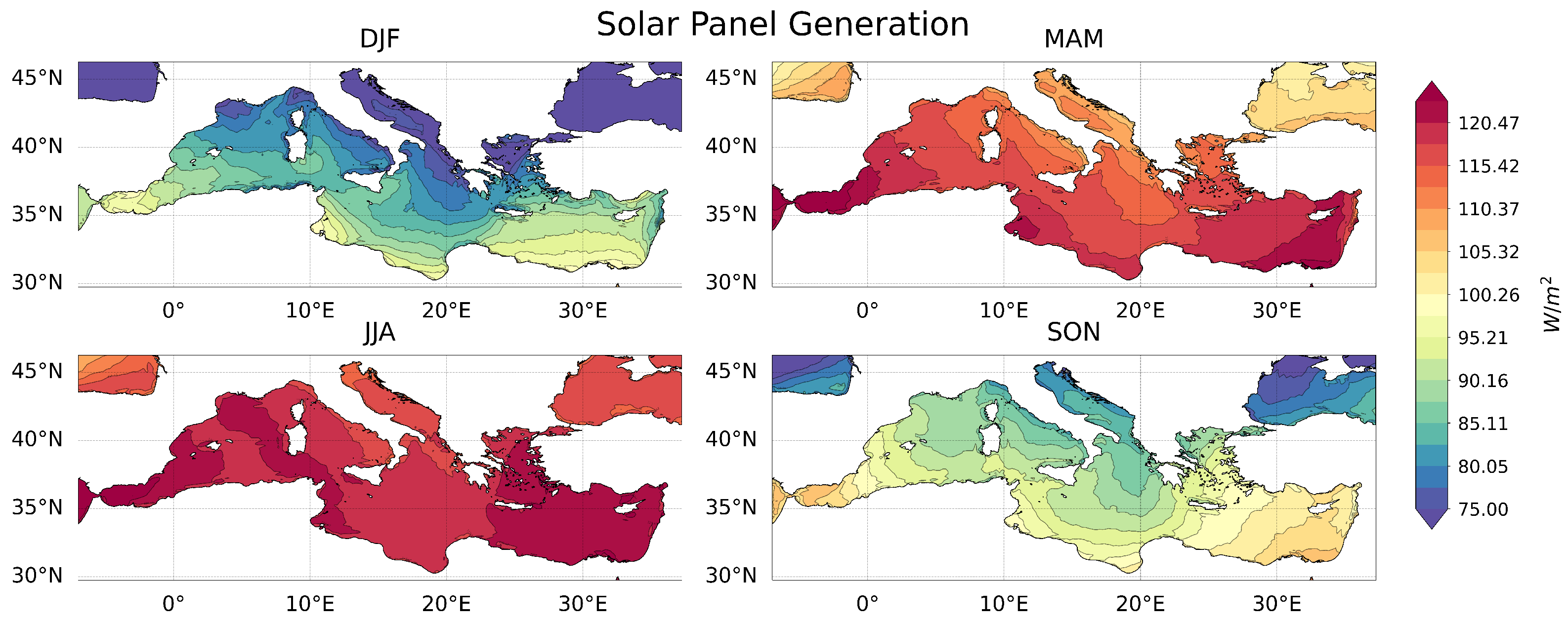
3.1.1. Solar
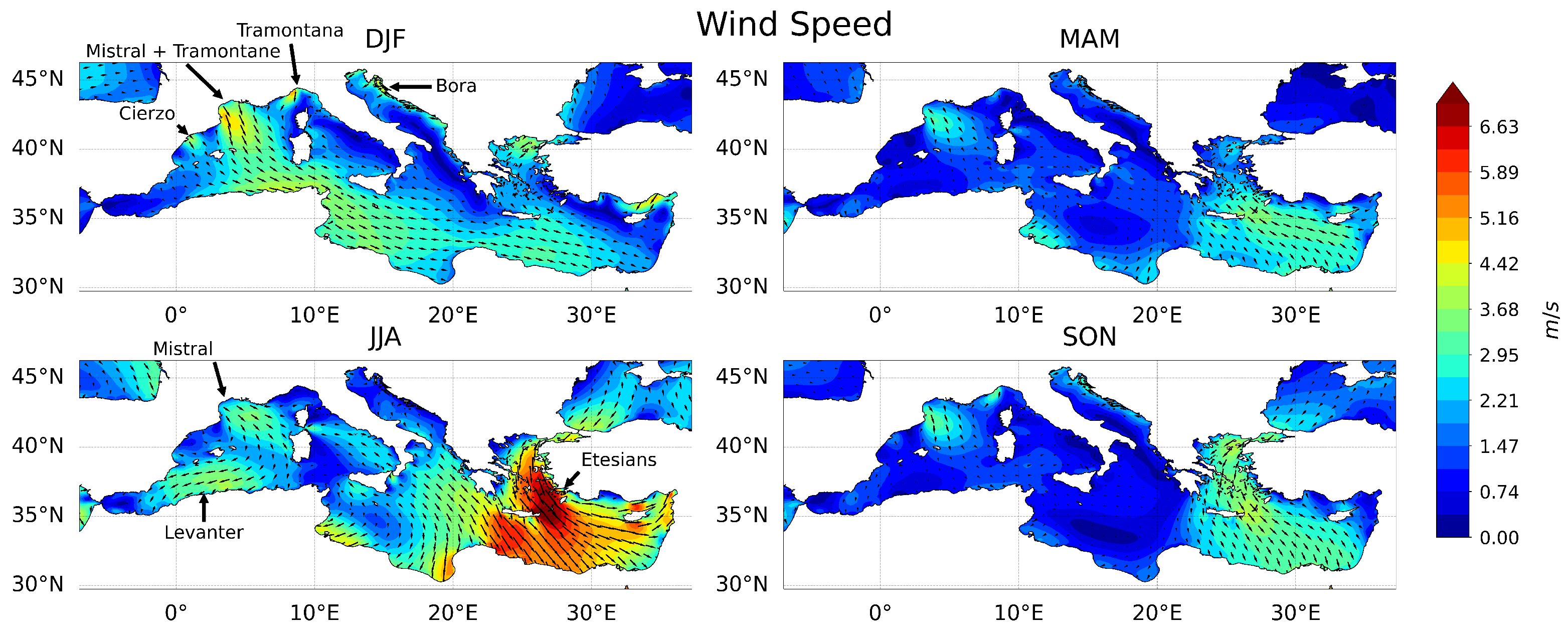
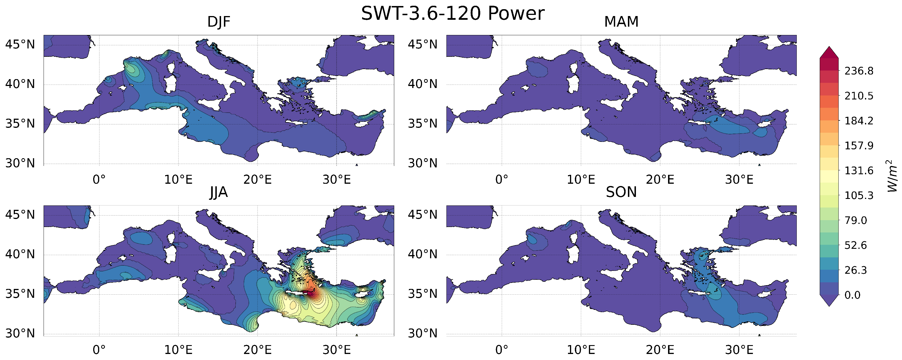
3.1.2. Wind
3.2. Environmental Risk
3.3. Methanol Production
Integrated Production
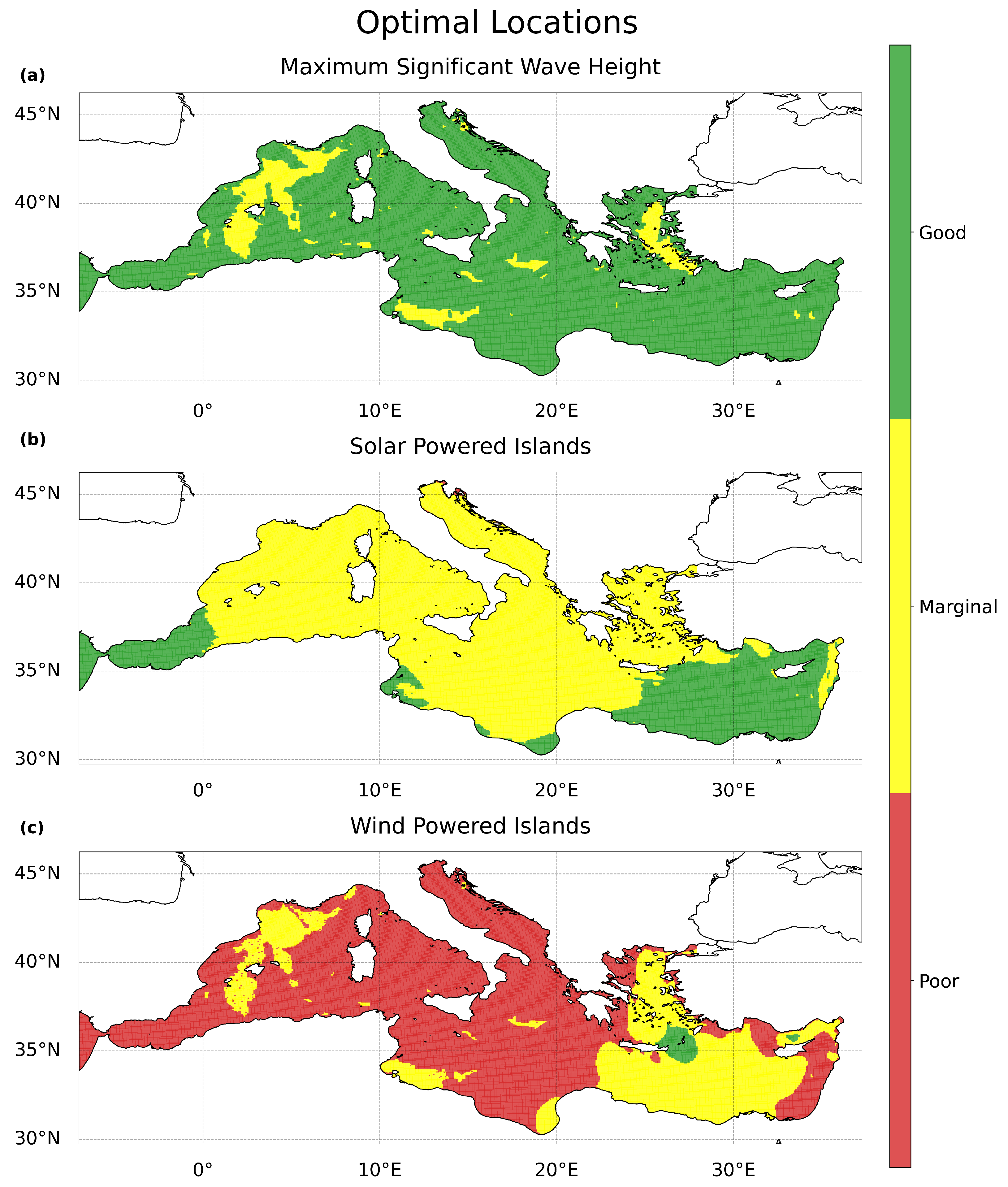
3.4. Optimal Locations
3.5. Remote and Island Communities
4. Conclusions
Author Contributions
Funding
Data Availability Statement
Acknowledgments
Conflicts of Interest
References
- United Nations Climate Change. The Paris Agreement. 2015. Available online: https://unfccc.int/process-and-meetings/the-paris-agreement/the-paris-agreement (accessed on 13 June 2022).
- de Coninck, H.; Revi, A.; Babiker, M.; Bertoldi, P.; Buckeridge, M.; Cartwright, A.; Dong, W.; Ford, J.; Fuss, S.; Hourcade, J.C.; et al. Strengthening and Implementing the Global Response. In Global Warming of 1.5 C; An IPCC Special Report on the impacts of global warming of 1.5 C above pre-industrial levels and related global greenhouse gas emission pathways, in the context of strengthening the global response to the threat of climate change, sustainable development, and efforts to eradicate poverty; Masson-Delmotte, V., Zhai, P., Pörtner, H.O., Roberts, D., Skea, J., Shukla, P., Pirani, A., Moufouma-Okia, W., Péan, C., Pidcock, R., et al., Eds.; Cambridge University Press: New York, NY, USA, 2018; Chapter 4; pp. 313–444. [Google Scholar] [CrossRef]
- Welch, A.J.; Digdaya, I.A.; Kent, R.; Ghougassian, P.; Atwater, H.A.; Xiang, C. Comparative Technoeconomic Analysis of Renewable Generation of Methane Using Sunlight, Water, and Carbon Dioxide. ACS Energy Lett. 2021, 6, 1540–1549. [Google Scholar] [CrossRef]
- Evans, S.G.; Ramage, B.S.; DiRocco, T.L.; Potts, M.D. Greenhouse Gas Mitigation on Marginal Land: A Quantitative Review of the Relative Benefits of Forest Recovery versus Biofuel Production. Environ. Sci. Technol. 2015, 49, 2503–2511. [Google Scholar] [CrossRef]
- Leung, D.Y.; Caramanna, G.; Maroto-Valer, M.M. An overview of current status of carbon dioxide capture and storage technologies. Renew. Sustain. Energy Rev. 2014, 39, 426–443. [Google Scholar] [CrossRef] [Green Version]
- Meylan, F.D.; Moreau, V.; Erkman, S. CO2 utilization in the perspective of industrial ecology, an overview. J. CO2 Util. 2015, 12, 101–108. [Google Scholar] [CrossRef]
- Bui, M.; Adjiman, C.S.; Bardow, A.; Anthony, E.J.; Boston, A.; Brown, S.; Fennell, P.S.; Fuss, S.; Galindo, A.; Hackett, L.A.; et al. Carbon capture and storage (CCS): The way forward. Energy Environ. Sci. 2018, 11, 1062–1176. [Google Scholar] [CrossRef] [Green Version]
- Renforth, P.; Jenkins, B.; Kruger, T. Engineering challenges of ocean liming. Energy 2013, 60, 442–452. [Google Scholar] [CrossRef] [Green Version]
- Fukuzumi, S.; Lee, Y.M.; Nam, W. Fuel Production from Seawater and Fuel Cells Using Seawater. ChemSusChem 2017, 10, 4264–4276. [Google Scholar] [CrossRef] [PubMed] [Green Version]
- Willauer, H.D.; DiMascio, F.; Hardy, D.R.; Williams, F.W. Development of an Electrolytic Cation Exchange Module for the Simultaneous Extraction of Carbon Dioxide and Hydrogen Gas from Natural Seawater. Energy Fuels 2017, 31, 1723–1730. [Google Scholar] [CrossRef]
- de Lannoy, C.F.; Eisaman, M.D.; Jose, A.; Karnitz, S.D.; DeVaul, R.W.; Hannun, K.; Rivest, J.L. Indirect ocean capture of atmospheric CO2: Part I. Prototype of a negative emissions technology. Int. J. Greenh. Gas Control 2018, 70, 243–253. [Google Scholar] [CrossRef]
- Sharifian, R.; Wagterveld, R.M.; Digdaya, I.A.; Xiang, C.; Vermaas, D.A. Electrochemical carbon dioxide capture to close the carbon cycle. Energy Environ. Sci. 2021, 14, 781–814. [Google Scholar] [CrossRef]
- Willauer, H.D.; Hardy, D.R.; Lewis, M.K.; Ndubizu, E.C.; Williams, F.W. Extraction of CO2 from Seawater and Aqueous Bicarbonate Systems by Ion-Exchange Resin Processes. Energy Fuels 2010, 24, 6682–6688. [Google Scholar] [CrossRef]
- Butenschön, M.; Lovato, T.; Masina, S.; Caserini, S.; Grosso, M. Alkalinization Scenarios in the Mediterranean Sea for Efficient Removal of Atmospheric CO2 and the Mitigation of Ocean Acidification. Front. Clim. 2021, 3, 1–11. [Google Scholar] [CrossRef]
- Greco-Coppi, M.; Hofmann, C.; Ströhle, J.; Walter, D.; Epple, B. Efficient CO2 capture from lime production by an indirectly heated carbonate looping process. Int. J. Greenh. Gas Control 2021, 112, 103430. [Google Scholar] [CrossRef]
- Tyka, M.D.; Arsdale, C.V.; Platt, J.C. CO2 capture by pumping surface acidity to the deep ocean. Energy Environ. Sci. 2022, 15, 786–798. [Google Scholar] [CrossRef]
- de Baar, H.J.W. Synthesis of iron fertilization experiments: From the Iron Age in the Age of Enlightenment. J. Geophys. Res. 2005, 110, 1–24. [Google Scholar] [CrossRef]
- Yoon, J.E.; Yoo, K.C.; Macdonald, A.M.; Yoon, H.I.; Park, K.T.; Yang, E.J.; Kim, H.C.; Lee, J.I.; Lee, M.K.; Jung, J.; et al. Reviews and syntheses: Ocean iron fertilization experiments–past, present, and future looking to a future Korean Iron Fertilization Experiment in the Southern Ocean (KIFES) project. Biogeosciences 2018, 15, 5847–5889. [Google Scholar] [CrossRef] [Green Version]
- Tripathy, S.C.; Jena, B. Iron-Stimulated Phytoplankton Blooms in the Southern Ocean: A Brief Review. Remote Sens. Earth Syst. Sci. 2019, 2, 64–77. [Google Scholar] [CrossRef]
- DiMascio, F.; Willauer, H.D.; Hardy, D.R.; Lewis, M.K.; Williams, F.W. Extraction of Carbon Dioxide from Seawater by an Electrochemical Acidification Cell Part I—Initial Feasibility Studies; Techreport NRL/MR/6180–10-9274; US Naval Research Laboratory: Washington, DC, USA, 2010. [Google Scholar]
- Willauer, H.D.; DiMascio, F.; Hardy, D.R.; Lewis, M.K.; Williams, F.W. Extraction of Carbon Dioxide from Seawater by an Electrochemical Acidification Cell Part II—Laboratory Scaling Studies; Techreport NRL/MR/6180–11-9329; US Naval Research Laboratory: Washington, DC, USA, 2011. [Google Scholar]
- Willauer, H.D.; DiMascio, F.; Hardy, D.R.; Lewis, M.K.; Williams, F.W. Development of an Electrochemical Acidification Cell for the Recovery of CO2 and H2 from Seawater. Ind. Eng. Chem. Res. 2011, 50, 9876–9882. [Google Scholar] [CrossRef]
- Willauer, H.D.; Hardy, D.R.; Williams, F.W.; DiMascio, F. Extraction of Carbon Dioxide and Hydrogen from Seawater by an Electrochemical Acidification Cell Part III—Scaled-Up Mobile Unit Studies (Calendar Year 2011); Techreport NRL/MR/6300–12-9414; US Naval Research Laboratory: Washington, DC, USA, 2012. [Google Scholar]
- Willauer, H.D.; Hardy, D.R.; Williams, F.W.; DiMascio, F. Extraction of Carbon Dioxide and Hydrogen from Seawater by an Electrochemical Acidification Cell Part IV—Electrode Compartments of Cell Modified and Tested in Scaled-Up Mobile Unit; Techreport NRL/MR/6300–13-9463; US Naval Research Laboratory: Washington, DC, USA, 2013. [Google Scholar]
- Willauer, H.D.; DiMascio, F.; Hardy, D.R.; Williams, F.W. Feasibility of CO2 Extraction from Seawater and Simultaneous Hydrogen Gas Generation Using a Novel and Robust Electrolytic Cation Exchange Module Based on Continuous Electrodeionization Technology. Ind. Eng. Chem. Res. 2014, 53, 12192–12200. [Google Scholar] [CrossRef]
- Willauer, H.D.; DiMascio, F.; Hardy, D.R. Extraction of Carbon Dioxide and Hydrogen from Seawater by an Electrolytic Cation Exchange Module (E-CEM) Part V—E-CEM Effluent Discharge Composition as a Function of Electrode Water Composition; Techreport NRL/MR/6360–17-9743; US Naval Research Laboratory: Washington, DC, USA, 2017. [Google Scholar]
- Eisaman, M.D.; Alvarado, L.; Larner, D.; Wang, P.; Littau, K.A. CO2 desorption using high-pressure bipolar membrane electrodialysis. Energy Environ. Sci. 2011, 4, 4031. [Google Scholar] [CrossRef]
- Eisaman, M.D.; Alvarado, L.; Larner, D.; Wang, P.; Garg, B.; Littau, K.A. CO2 separation using bipolar membrane electrodialysis. Energy Environ. Sci. 2011, 4, 1319–1328. [Google Scholar] [CrossRef]
- Eisaman, M.D.; Parajuly, K.; Tuganov, A.; Eldershaw, C.; Chang, N.; Littau, K.A. CO2 extraction from seawater using bipolar membrane electrodialysis. Energy Environ. Sci. 2012, 5, 7346–7352. [Google Scholar] [CrossRef] [Green Version]
- Eisaman, M.D.; Rivest, J.L.; Karnitz, S.D.; de Lannoy, C.F.; Jose, A.; DeVaul, R.W.; Hannun, K. Indirect ocean capture of atmospheric CO2: Part II. Understanding the cost of negative emissions. Int. J. Greenh. Gas Control 2018, 70, 254–261. [Google Scholar] [CrossRef]
- Willauer, H.D.; Hardy, D.R.; Schultz, K.R.; Williams, F.W. The feasibility and current estimated capital costs of producing jet fuel at sea using carbon dioxide and hydrogen. J. Renew. Sustain. Energy 2012, 4, 033111. [Google Scholar] [CrossRef] [Green Version]
- Patterson, B.D.; Mo, F.; Borgschulte, A.; Hillestad, M.; Joos, F.; Kristiansen, T.; Sunde, S.; van Bokhoven, J.A. Renewable CO2 recycling and synthetic fuel production in a marine environment. Proc. Natl. Acad. Sci. USA 2019, 116, 12212–12219. [Google Scholar] [CrossRef] [PubMed] [Green Version]
- Terreni, J.; Borgschulte, A.; Hillestad, M.; Patterson, B.D. Understanding Catalysis—A Simplified Simulation of Catalytic Reactors for CO2 Reduction. ChemEngineering 2020, 4, 62. [Google Scholar] [CrossRef]
- Digdaya, I.A.; Sullivan, I.; Lin, M.; Han, L.; Cheng, W.H.; Atwater, H.A.; Xiang, C. A direct coupled electrochemical system for capture and conversion of CO2 from oceanwater. Nat. Commun. 2020, 11, 4412. [Google Scholar] [CrossRef] [PubMed]
- Sahu, A.; Yadav, N.; Sudhakar, K. Floating photovoltaic power plant: A review. Renew. Sustain. Energy Rev. 2016, 66, 815–824. [Google Scholar] [CrossRef]
- Drobinski, P.; Azzopardi, B.; Allal, H.B.J.; Bouchet, V.; Civel, E.; Creti, A.; Duic, N.; Fylaktos, N.; Mutale, J.; Pariente-David, S.; et al. Energy transition in the Mediterranean. In Climate and Environmental Change in the Mediterranean Basin—Current Situation and Risks for the Future; Union for the Mediterranean, Plan Bleu, UNEP/MAP: Marseille, France, 2020; Chapter 3; pp. 265–322. [Google Scholar]
- Soukissian, T.; Denaxa, D.; Karathanasi, F.; Prospathopoulos, A.; Sarantakos, K.; Iona, A.; Georgantas, K.; Mavrakos, S. Marine Renewable Energy in the Mediterranean Sea: Status and Perspectives. Energies 2017, 10, 1512. [Google Scholar] [CrossRef]
- Drobinski, P.; Alpert, P.; Cavicchia, L.; Flaounas, E.; Hochman, A.; Kotroni, V. Strong Winds: Observed Trends, Future Projections, in The Mediterranean Region under Climate Change—A Scientific Update; IRD Editions: Montpellier, France, 2016; Chapter 1; pp. 115–122. [Google Scholar]
- Overpeck, J.T.; Meehl, G.A.; Bony, S.; Easterling, D.R. Climate Data Challenges in the 21st Century. Science 2011, 331, 700–702. [Google Scholar] [CrossRef]
- Medeiros, D. DWSIM. Software. 2022. Available online: https://dwsim.org (accessed on 22 November 2022).
- Guion, A.; Turquety, S.; Polcher, J.; Pennel, R.; Bastin, S.; Arsouze, T. Droughts and heatwaves in the Western Mediterranean: Impact on vegetation and wildfires using the coupled WRF-ORCHIDEE regional model (RegIPSL). Clim. Dyn. 2021, 58, 2881–2903. [Google Scholar] [CrossRef]
- Skamarock, W.; Klemp, J.; Dudhia, J.; Gill, D.; Barker, D.; Wang, W.; Huang, X.Y.; Duda, M. A Description of the Advanced Research WRF Version 3; Technical Report; UCAR/NCAR: Boulder, CO, USA, 2008. [Google Scholar] [CrossRef]
- Krinner, G.; Viovy, N.; de Noblet-Ducoudré, N.; Ogée, J.; Polcher, J.; Friedlingstein, P.; Ciais, P.; Sitch, S.; Prentice, I.C. A dynamic global vegetation model for studies of the coupled atmosphere-biosphere system. Glob. Biogeochem. Cycles 2005, 19, GB1015. [Google Scholar] [CrossRef]
- Ruti, P.M.; Somot, S.; Giorgi, F.; Dubois, C.; Flaounas, E.; Obermann, A.; Dell’Aquila, A.; Pisacane, G.; Harzallah, A.; Lombardi, E.; et al. Med-CORDEX Initiative for Mediterranean Climate Studies. Bull. Am. Meteorol. Soc. 2016, 97, 1187–1208. [Google Scholar] [CrossRef] [Green Version]
- Waldman, R.; Brüggemann, N.; Bosse, A.; Spall, M.; Somot, S.; Sevault, F. Overturning the Mediterranean Thermohaline Circulation. Geophys. Res. Lett. 2018, 45, 8407–8415. [Google Scholar] [CrossRef] [Green Version]
- Hamon, M.; Beuvier, J.; Somot, S.; Lellouche, J.M.; Greiner, E.; Jordà, G.; Bouin, M.N.; Arsouze, T.; Béranger, K.; Sevault, F.; et al. Design and validation of MEDRYS, a Mediterranean Sea reanalysis over the period 1992–2013. Ocean Sci. 2016, 12, 577–599. [Google Scholar] [CrossRef] [Green Version]
- Beuvier, J.; Béranger, K.; Brossier, C.L.; Somot, S.; Sevault, F.; Drillet, Y.; Bourdallé-Badie, R.; Ferry, N.; Lyard, F. Spreading of the Western Mediterranean Deep Water after winter 2005: Time scales and deep cyclone transport. J. Geophys. Res. Ocean. 2012, 117, 1–26. [Google Scholar] [CrossRef]
- Lebeaupin-Brossier, C.; Béranger, K.; Deltel, C.; Drobinski, P. The Mediterranean response to different space–time resolution atmospheric forcings using perpetual mode sensitivity simulations. Ocean Model. 2011, 36, 1–25. [Google Scholar] [CrossRef]
- Balmaseda, M.A.; Trenberth, K.E.; Källén, E. Distinctive climate signals in reanalysis of global ocean heat content. Geophys. Res. Lett. 2013, 40, 1754–1759. [Google Scholar] [CrossRef]
- Ludwig, W.; Dumont, E.; Meybeck, M.; Heussner, S. River discharges of water and nutrients to the Mediterranean and Black Sea: Major drivers for ecosystem changes during past and future decades? Prog. Oceanogr. 2009, 80, 199–217. [Google Scholar] [CrossRef]
- Holmgren, W.F.; Hansen, C.W.; Mikofski, M.A. pvlib python: A python package for modeling solar energy systems. J. Open Source Softw. 2018, 3, 884. [Google Scholar] [CrossRef] [Green Version]
- Maxwell, E.L. A Quasi-Physical Model for Converting Hourly Global Horizontal to Direct Normal Insolation; Technical Report; Solar Energy Research Institute: Golden, CO, USA, 1987. [Google Scholar]
- Kratochvil, J.; Boyson, W.; King, D. Photovoltaic Array Performance Model; Technical Report; Sandia National Laboratories: Albuquerque, NM, USA; Livermore, CA, USA, 2004. [Google Scholar] [CrossRef] [Green Version]
- Manwell, J.F. Wind Energy Explained; Wiley: Chichester, UK, 2009; Chapter 2.3.4.1; pp. 1–689. [Google Scholar]
- Arshad, M.; O’Kelly, B.C. Offshore wind-turbine structures: A review. Proc. Inst. Civ. Eng. Energy 2013, 166, 139–152. [Google Scholar] [CrossRef]
- Haas, S.; Krien, U.; Schachler, B.; Bot, S.; Kyri-Petrou; Zeli, V.; Shivam, K.; Bosch, S. Wind-Python/Windpowerlib: Silent Improvements (v0.2.1); Zenodo: Geneva, Switzerland, 2021. [Google Scholar] [CrossRef]
- World Meteorological Organization. Guide to Wave Analysis and Forecasting; Secretariat of the World Meteorological Organization: Geneva, Switzerland, 2018. [Google Scholar]
- Lueker, T.J.; Dickson, A.G.; Keeling, C.D. Ocean pCO2 calculated from dissolved inorganic carbon, alkalinity, and equations for K1 and K2: Validation based on laboratory measurements of CO2 in gas and seawater at equilibrium. Mar. Chem. 2000, 70, 105–119. [Google Scholar] [CrossRef]
- Wang, L.; Violet, C.; DuChanois, R.M.; Elimelech, M. Derivation of the Theoretical Minimum Energy of Separation of Desalination Processes. J. Chem. Educ. 2020, 97, 4361–4369. [Google Scholar] [CrossRef]
- Shen, M.; Bennett, N.; Ding, Y.; Scott, K. A concise model for evaluating water electrolysis. Int. J. Hydrog. Energy 2011, 36, 14335–14341. [Google Scholar] [CrossRef] [Green Version]
- Givon, Y.; Keller, D., Jr.; Silverman, V.; Pennel, R.; Drobinski, P.; Raveh-Rubin, S. Large-scale drivers of the mistral wind: Link to Rossby wave life cycles and seasonal variability. Weather Clim. Dyn. 2021, 2, 609–630. [Google Scholar] [CrossRef]
- Jurčec, V. On mesoscale characteristics of bora conditions in Yugoslavia. Pure Appl. Geophys. PAGEOPH 1980, 119, 640–657. [Google Scholar] [CrossRef]
- Drobinski, P.; Flamant, C.; Dusek, J.; Flamant, P.H.; Pelon, J. Observational Evidence And Modelling Of An Internal Hydraulic Jump At The Atmospheric Boundary-Layer Top During A Tramontane Event. Bound.-Layer Meteorol. 2001, 98, 497–515. [Google Scholar] [CrossRef]
- Drobinski, P.; Alonzo, B.; Basdevant, C.; Cocquerez, P.; Doerenbecher, A.; Fourrié, N.; Nuret, M. Lagrangian dynamics of the mistral during the HyMeX SOP2. J. Geophys. Res. Atmos. 2017, 122, 1387–1402. [Google Scholar] [CrossRef]
- Zecchetto, S.; Biasio, F.D. Sea Surface Winds over the Mediterranean Basin from Satellite Data (2000–04): Meso- and Local-Scale Features on Annual and Seasonal Time Scales. J. Appl. Meteorol. Climatol. 2007, 46, 814–827. [Google Scholar] [CrossRef]
- Masson, V.; Bougeault, P. Numerical Simulation of a Low-Level Wind Created by Complex Orography: A Cierzo Case Study. Mon. Weather Rev. 1996, 124, 701–715. [Google Scholar] [CrossRef]
- Drobinski, P.; Bastin, S.; Guenard, V.; Caccia, J.L.; Dabas, A.; Delville, P.; Protat, A.; Reitebuch, O.; Werner, C. Summer mistral at the exit of the Rhône valley. Q. J. R. Meteorol. Soc. 2005, 131, 353–375. [Google Scholar] [CrossRef] [Green Version]
- Ziv, B.; Saaroni, H.; Alpert, P. The factors governing the summer regime of the eastern Mediterranean. Int. J. Climatol. 2004, 24, 1859–1871. [Google Scholar] [CrossRef]
- Kaymak, M.K.; Şahin, A.D. Problems encountered with floating photovoltaic systems under real conditions: A new FPV concept and novel solutions. Sustain. Energy Technol. Assess. 2021, 47, 101504. [Google Scholar] [CrossRef]
- Martini, M.; Guanche, R.; Armesto, J.A.; Losada, I.J.; Vidal, C. Met-ocean conditions influence on floating offshore wind farms power production. Wind Energy 2015, 19, 399–420. [Google Scholar] [CrossRef]
- Galanis, G.; Hayes, D.; Zodiatis, G.; Chu, P.C.; Kuo, Y.H.; Kallos, G. Wave height characteristics in the Mediterranean Sea by means of numerical modeling, satellite data, statistical and geometrical techniques. Mar. Geophys. Res. 2011, 33, 1–15. [Google Scholar] [CrossRef] [Green Version]
- Millet, P.; Ngameni, R.; Grigoriev, S.; Mbemba, N.; Brisset, F.; Ranjbari, A.; Etiévant, C. PEM water electrolyzers: From electrocatalysis to stack development. Int. J. Hydrog. Energy 2010, 35, 5043–5052. [Google Scholar] [CrossRef]
- Skrzypek, J.; Lachowska, M.; Serafin, D. Methanol synthesis from CO2 and H2: Dependence of equilibrium conversions and exit equilibrium concentrations of components on the main process variables. Chem. Eng. Sci. 1990, 45, 89–96. [Google Scholar] [CrossRef]
- Grigoriev, S.; Fateev, V.; Bessarabov, D.; Millet, P. Current status, research trends, and challenges in water electrolysis science and technology. Int. J. Hydrog. Energy 2020, 45, 26036–26058. [Google Scholar] [CrossRef]
- Ramachandran, R.C.; Desmond, C.; Judge, F.; Serraris, J.J.; Murphy, J. Floating wind turbines: Marine operations challenges and opportunities. Wind Energy Sci. 2022, 7, 903–924. [Google Scholar] [CrossRef]
- Cauz, M.; Bloch, L.; Rod, C.; Perret, L.; Ballif, C.; Wyrsch, N. Benefits of a Diversified Energy Mix for Islanded Systems. Front. Energy Res. 2020, 8, 1–8. [Google Scholar] [CrossRef]
- Vourdoubas, J. Studies on the Electrification of the Transport Sector in the Island of Crete, Greece. Open J. Energy Effic. 2018, 07, 19–32. [Google Scholar] [CrossRef] [Green Version]
- Ginard-Bosch, F.J.; Ramos-Martín, J. Energy metabolism of the Balearic Islands (1986–2012). Ecol. Econ. 2016, 124, 25–35. [Google Scholar] [CrossRef]
- Álvarez, M.; Sanleón-Bartolomé, H.; Tanhua, T.; Mintrop, L.; Luchetta, A.; Cantoni, C.; Schroeder, K.; Civitarese, G. The CO2 system in the Mediterranean Sea: A basin wide perspective. Ocean Sci. 2014, 10, 69–92. [Google Scholar] [CrossRef] [Green Version]
- Berger, M.; Bopp, L.; Ho, D.T.; Kwiatkowski, L. Assessing global macroalgal carbon dioxide removal potential using a high-resolution ocean biogeochemistry model. In Proceedings of the EGU General Assembly 2022, EGU22-4699, Vienna, Austria, 23–27 May 2022. [Google Scholar] [CrossRef]
- Riebesell, U.; Wolf-Gladrow, D.A.; Smetacek, V. Carbon dioxide limitation of marine phytoplankton growth rates. Nature 1993, 361, 249–251. [Google Scholar] [CrossRef]
- Kroeker, K.J.; Kordas, R.L.; Crim, R.; Hendriks, I.E.; Ramajo, L.; Singh, G.S.; Duarte, C.M.; Gattuso, J.P. Impacts of ocean acidification on marine organisms: Quantifying sensitivities and interaction with warming. Glob. Chang. Biol. 2013, 19, 1884–1896. [Google Scholar] [CrossRef] [PubMed]
- Haigh, R.; Ianson, D.; Holt, C.A.; Neate, H.E.; Edwards, A.M. Effects of Ocean Acidification on Temperate Coastal Marine Ecosystems and Fisheries in the Northeast Pacific. PLoS ONE 2015, 10, e0117533. [Google Scholar] [CrossRef] [PubMed]
- Heinze, C.; Meyer, S.; Goris, N.; Anderson, L.; Steinfeldt, R.; Chang, N.; Quéré, C.L.; Bakker, D.C.E. The ocean carbon sink–impacts, vulnerabilities and challenges. Earth Syst. Dyn. 2015, 6, 327–358. [Google Scholar] [CrossRef] [Green Version]
- Lacoue-Labarthe, T.; Nunes, P.A.; Ziveri, P.; Cinar, M.; Gazeau, F.; Hall-Spencer, J.M.; Hilmi, N.; Moschella, P.; Safa, A.; Sauzade, D.; et al. Impacts of ocean acidification in a warming Mediterranean Sea: An overview. Reg. Stud. Mar. Sci. 2016, 5, 1–11. [Google Scholar] [CrossRef] [Green Version]
- Flecha, S.; Pérez, F.F.; García-Lafuente, J.; Sammartino, S.; Ríos, A.F.; Huertas, I.E. Trends of pH decrease in the Mediterranean Sea through high frequency observational data: Indication of ocean acidification in the basin. Sci. Rep. 2015, 5, 16770. [Google Scholar] [CrossRef] [PubMed] [Green Version]
- Keller, D.P.; Lenton, A.; Littleton, E.W.; Oschlies, A.; Scott, V.; Vaughan, N.E. The Effects of Carbon Dioxide Removal on the Carbon Cycle. Curr. Clim. Chang. Rep. 2018, 4, 250–265. [Google Scholar] [CrossRef] [Green Version]
- Keller, D.P.; Lenton, A.; Scott, V.; Vaughan, N.E.; Bauer, N.; Ji, D.; Jones, C.D.; Kravitz, B.; Muri, H.; Zickfeld, K. The Carbon Dioxide Removal Model Intercomparison Project (CDRMIP): Rationale and experimental protocol for CMIP6. Geosci. Model Dev. 2018, 11, 1133–1160. [Google Scholar] [CrossRef]


| Input and State Parameters | ||||
|---|---|---|---|---|
| Degasser | ||||
| Seawater inflow (L s−1) | ||||
| 10 | ||||
| Desalinator | ||||
| Seawater inflow (L s−1) | n stages | |||
| 0.01 | 0.5 | 1 | 0.99 | |
| Electrolyzer | ||||
| (V) | R ( cm−2) | K ( cm−2) | (cm2) | |
| 1.4 | 0.15 | 27.8 | 250 | |
| Reactor | ||||
| T (°C) | P (bars) | (m2) | (m) | (kg m−3) |
| 180 | 60 | 3.14 | 3 | 1000 |
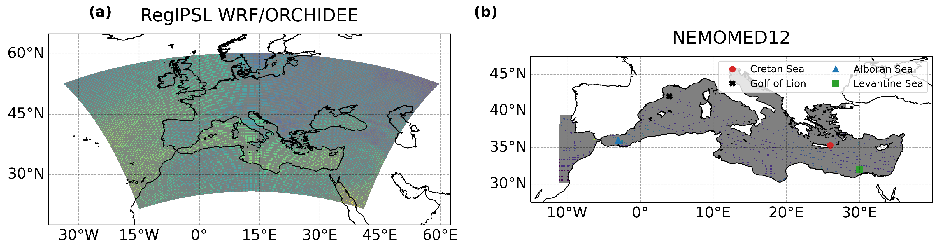
| Location | Alboran Sea | Gulf of Lion | Cretan Sea | Levantine Sea |
|---|---|---|---|---|
| Coordinates | 36° N 3° W | 42° N 4° E | 35.30° N 26° E | 32° N 30° E |
| Max Wave Height (m) | 1.54 | 2.54 | 1.55 | 1.36 |
| Integrated Methanol Production (mL/m2) | ||||
| Solar | 494.21 | 445.52 | 465.10 | 484.70 |
| Wind | 20.80 | 219.60 | 457.29 | 152.85 |
Publisher’s Note: MDPI stays neutral with regard to jurisdictional claims in published maps and institutional affiliations. |
© 2022 by the authors. Licensee MDPI, Basel, Switzerland. This article is an open access article distributed under the terms and conditions of the Creative Commons Attribution (CC BY) license (https://creativecommons.org/licenses/by/4.0/).
Share and Cite
Keller, D., Jr.; Somanna, V.; Drobinski, P.; Tard, C. Offshore CO2 Capture and Utilization Using Floating Wind/PV Systems: Site Assessment and Efficiency Analysis in the Mediterranean. Energies 2022, 15, 8873. https://doi.org/10.3390/en15238873
Keller D Jr., Somanna V, Drobinski P, Tard C. Offshore CO2 Capture and Utilization Using Floating Wind/PV Systems: Site Assessment and Efficiency Analysis in the Mediterranean. Energies. 2022; 15(23):8873. https://doi.org/10.3390/en15238873
Chicago/Turabian StyleKeller, Douglas, Jr., Vishal Somanna, Philippe Drobinski, and Cédric Tard. 2022. "Offshore CO2 Capture and Utilization Using Floating Wind/PV Systems: Site Assessment and Efficiency Analysis in the Mediterranean" Energies 15, no. 23: 8873. https://doi.org/10.3390/en15238873