
Time vs. Capacity—The Potential of Optimal Charging Stop Strategies for Battery Electric Trucks


Institute of Automotive Technology, Technical University Munich, Boltzmannstraße 15, 85748 Garching, Germany
*
Author to whom correspondence should be addressed.
Energies 2022, 15(19), 7137; https://doi.org/10.3390/en15197137
Submission received: 13 September 2022
/
Revised: 23 September 2022
/
Accepted: 25 September 2022
/
Published: 28 September 2022
(This article belongs to the Topic Advanced Electric Vehicle Technology)
Abstract
:The decarbonization of the transport sector, and thus of road-based transport logistics, through electrification, is essential to achieve European climate targets. Battery electric trucks offer the greatest well-to-wheel potential for CO2 saving. At the same time, however, they are subject to restrictions due to charging events because of their limited range compared to conventional trucks. These restrictions can be kept to a minimum through optimal charging stop strategies. In this paper, we quantify these restrictions and show the potential of optimal strategies. The modeling of an optimal charging stop strategy is described mathematically as an optimization problem and solved by a genetic algorithm. The results show that in the case of long-distance transport using trucks with battery capacities lower than 750 kWh, a time loss is to be expected. However, this can be kept below 20 min for most battery capacities by optimal charging stops and sufficient charging infrastructure.
1. Introduction
Transport logistics is the backbone of the global economy, but also contributes significantly to CO2 emissions [1]; e.g., road-based transport logistics accounts for 38% of total emissions caused by the transport sector in the European Union in 2019 [2]. In response to the global climate crises, the European Union has set a CO2 reduction target of 30% for commercial vehicles by 2030 compared to 2019 [3]. Such emission reductions can be achieved by fully electrified, so-called zero-emission trucks [4]. The two priority powertrain concepts for this are battery electric trucks (BET) and fuel cell electric trucks (FCET). Due to the significantly higher well-to-wheel efficiency, BET offer the highest potential for overall emission reduction [5,6]. In addition, studies indicate that BET offer cost advantages over FCET due to their higher well-to-wheel efficiency [7,8,9]. Therefore, in this paper we focus on BET.
Long-distance transport, which is responsible for 70% of CO2 emissions in European road-based transport logistics [2], offers great potential for reducing emission in road freight transport. However, due to the high, daily milage of over 350 km, this sector is difficult to electrify by BET. The central hurdle is the currently possible range, resulting from a limited battery capacity both for payload and package reasons. A limited range leads to necessary charging events during the journey. From a technological point of view, the newly defined Megawatt Charging System (MCS) provides a remedy [10]. According to this standard, a charging power of over 1 MW is available in the future for fast charging of BET [11]. However, it has not yet been clarified whether and what time loss must be expected for battery electric vehicles compared to internal combustion engine trucks (ICET), even when using such a high charging power. The time loss must be quantifiable and acceptable for principle integrability into existing logistic processes.
A second hurdle is the high investment costs of BET compared to ICET at the beginning of the utilization phase. For the desired long ranges, therefore needing less charging events, high battery capacities are needed, leading to high investment costs [12]. In summary, we identify two coupled challenges from an operational point of view for BET:
- When integrated into existing logistic process, restrictions due to charging events and consequently a loss of time compared to ICET should be expected. The magnitude of the time loss depends on the battery capacity and charging power but is yet unknown. The higher the battery capacity, the fewer charging events are needed.
- For long ranges and thus a mitigation of the first challenge, high investment costs and a lower payload must be expected.
The coupling of both challenges leads to the conflicting goals of low investment costs and thus low battery capacity and the lowest restrictions due the charging events. This trade-off is addressed by the operational strategy of BET. By operational strategy, we mean the optimal charging stop strategy for a specific freight mission. One goal of such a strategy should be to minimize the total time required to complete the freight task and consequently minimize the time loss compared to ICET. An increasing duration leads to a decrease in the annual transport performance and consequently to an increase in the total cost of ownership (TCO). Furthermore, the driver has to be paid for a longer period, which increases TCO, too. Due to the legally prescribed rest times in Europe, there is the possibility to use these for charging events. Accordingly, a 45-min rest must be taken after 4.5 h of driving. A division into 15 and 30 min is also permissible [13].
The optimal planning of the charging stops and their integration into mandatory rest schedules requires a large amount of system information and predictions, such as the State of Charge (SoC) or occupancy of the charging points. Current stressor of truck drivers, such as tight time constraints or finding a parking space, already make the job unattractive today [14,15]. The transformation to BET would add a new stress: searching for optimal charging points. This must be avoided by proposing an optimal and reliable strategy to the driver that integrates the necessary charging events in an optimal way. The definition of optimality depends on the freight task and can include both time and monetary aspects. Therefore, we derive the following research questions, which we try to answer within the scope of this paper.
- What is the potential of an optimal charging stop strategy compared to just not getting stranded?
- What time loss can be expected when using an optimal charging stop strategy depending on battery capacity?
- What influence do the charging infrastructure characteristics, such as charging power, have on optimal strategies?
- In general, the planning and optimization of charging stops can be investigated by two different approaches, which are presented next.
2. Approaches for Charging Stop Consideration and Optimization
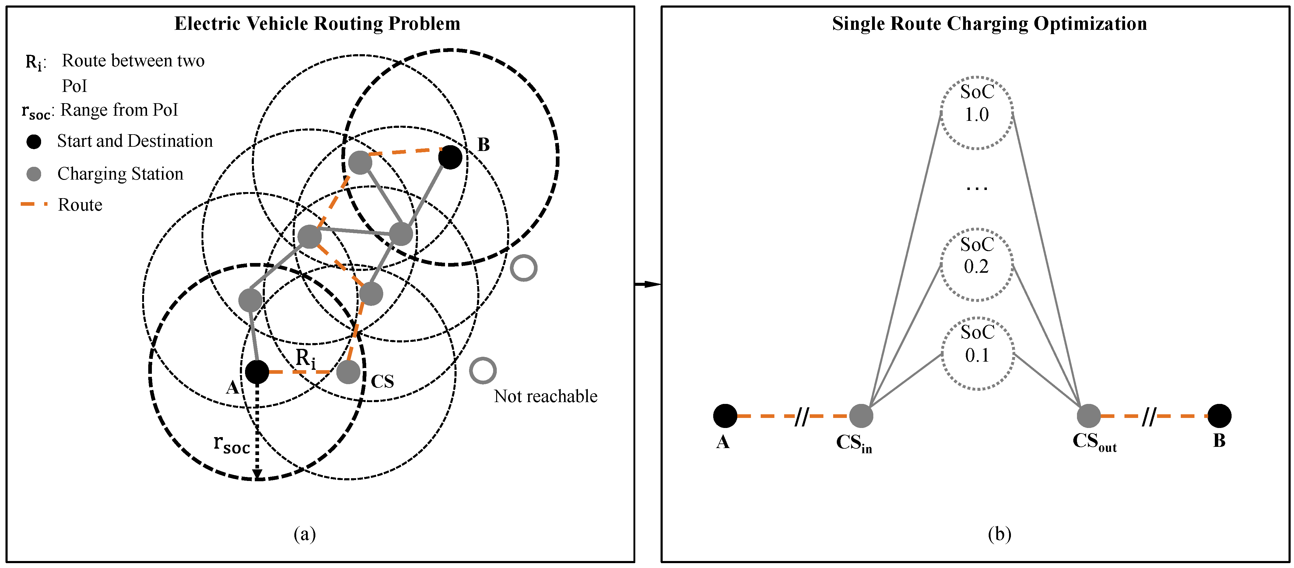
The consideration of battery electric vehicles in the well-known vehicle routing problem (VRP) leads to the electric vehicle problem (EVRP). In general, the objective is to find an optimal route in a network of (local) nodes [16]. Optimal can mean energy, cost, or time efficient. Likewise, these nodes can provide a charging possibility, so that a charging strategy can be considered in the context of EVRPs (Figure 1a). This approach is contrasted with the concrete charging stop optimization for an already known route. Here, too, a graph can be constructed, whereby the nodes do not describe a location, but define a different State of Charge (SoC) level up to which charging can be performed (Figure 1b).
The single-route approach can be seen as a downstream step of the EVRP. Once an optimal route has been found, the charging strategy can be optimized for it. Through simplifications, charging events can already be taken into account during the route finding. However, for finding a coupled optimal solution for route and strategy, a graph can be generated that connects each node in Figure 1a with the graph in Figure 1b. In addition to the resulting network size, non-linear properties, such as the charging behavior of the vehicle battery, make a solution even for static conditions almost impossible [17,19].
2.1. Electric Vehicle Routing Considerations
A broad overview of different variants of EVRPs is given by Erdlić et al. [20]. Therefore, we address below aspects that specifically affect charging within the EVRP. Due to their recuperation capability, BEV offer the feature that the energy consumption on route sections can be negative; the battery is therefore charged and thus the classical routing methods, such as the Dijkstra [21] algorithms, cannot be applied without further adjustments [20,22]. To address this, Artmeier et al. [22] show how the classical shortest path problem for BEV can be transformed into an energy-efficient routing problem. By using the negative weights of edges, due to recuperation, in an routable energy consumption-based graph, BEV charging is considered here in a figurative sense [22]. Storandt et al. [23] built on this work and showed advanced algorithms that can be applied to larger routing networks.
The first integration of concrete charging points into the electric vehicle routing problem (EVRP) was performed by Kobayashi et al. [17]. In their approach, relevant charging points in the network are searched first, which result from overlapping regions related to the range of starting, the destination point, and possible charging nodes [17]. Once these are identified, ordinary routing algorithms are applied to find routes between the different points of interest (PoIs). The final route is obtained as the best combination of the individual routes (Figure 1a). Kobayashi et al. [17] made the simplification to fully charge the vehicle at the charging points and assume linear battery-charging behavior.
Both simplifications were dropped by Sweda et al. [19]. In their approach, they considered the non-linear charging behavior of the battery as well as the possibility of incomplete charging processes. For this purpose, in a first step, the complexity is reduced to the extent that charging takes place along a route at each node. For the optimized charging strategy in the second step, Sweda et al. [19] provide a dynamic programing approach. A nearly similar approach was taken by Cassandras et al. [24] but with the goal of minimizing the total travel time rather than energy consumption. This also includes minimizing the charging time without getting stranded during the trip. Analogously, they divide the problem of routing and the optimal charging amount into two subproblems. However, this decomposition is only possible for linear battery-charging behavior when minimizing the total time. In contrast to the single-vehicle consideration presented so far, Schneider et al. [25] show the extension to fleets with the goal of minimizing the total number of vehicles and the total route length.
The integration of a charging strategy into VRP is limited by the increasing complexity of large networks, additional decision variables such as travel speed on edges, or the consideration of dynamic events. Therefore, the primary research objective is to consider the objective of an optimal charging strategy detached from routing by assuming a predefined route.
2.2. Single-Route Charging Optimization
Starting with a known route and its charging infrastructure, Huber et al. [18] showed a charging strategy optimization approach taking into account temporal and local traffic information as well as non-linear charging behavior. The optimization problem is modeled as a directed graph for a defined route. For this purpose, a discretization of the possible SoC level after the charging cycle was performed. Branches of the graph at the positions of the charging points allow this option of different charging levels (Figure 1b). As a solution method, they showed an adapted Dijkstra algorithm [18]. In further work, Huber et al. [26] showed the integration of a dynamic energy buffer to react to unforeseen effects, which locally mean higher energy consumption.
To minimize the total travel time, charging stops can also be avoided by a lower travel speed and consequently lower energy consumption. Cussigh et al. [27] showed for the first time an optimized driving and charging strategy by introducing the speed between two nodes on a predefined route as an additional design variable. A dynamic programing approach was used as the solution method [27]. Based on the two general approaches for charging stop consideration and the research questions formulated before, we derive the research gap below.
2.3. Research Gap
The focus of charging strategy optimization in research to date has been on passenger cars and small commercial vehicles that are not linked to mandatory rest schedules. This circumstance is fundamentally different from passenger cars since the goal now is to optimally integrate charging events into prescribed driving breaks. This has not been shown in the literature so far. At a point of interest (PoI), both the desired SoC and the end of the charging event, as well as the optimal rest time, must be determined, where a PoI is a rest site with or without a charging possibility. The consideration of this coupling will be shown for the first time in this paper. For a known route with 10 PoIs, a discretization of the SoC level in 10 steps, and 3 possible rest times (e.g., 15, 30, 45 min), the coupling of charging and resting leads to possible strategies (Figure 1b), with 300 nodes. The solution of such problems results in high computational effort, so that it should be clarified which potential an optimal strategy has at all. Therefore, we will focus here on the single-route consideration of charging stop strategies. To address this, we present in the following the proposed methodology.
3. Methodology for the Potential Analysis of an Optimal Charging Stop Strategy for BET
To answer the research questions derived in the beginning, we show in this paper the potential of an optimal charging stop strategy for BET. For reference, we adopt a strategy whose goal is only to not get stranded. We refer to this as the Not Getting Stranded strategy (NGS). This is contrasted with the Fully Optimized strategy (FO), whose objective is the minimum total travel time of the underlying freight mission. To evaluate these strategies shown in this section, we need to simulate the operation of a BET in its environment. For this purpose, we first present the modeling approach of the simulation environment and its models followed by the mentioned charging stop strategies.
3.1. Simulation Environment
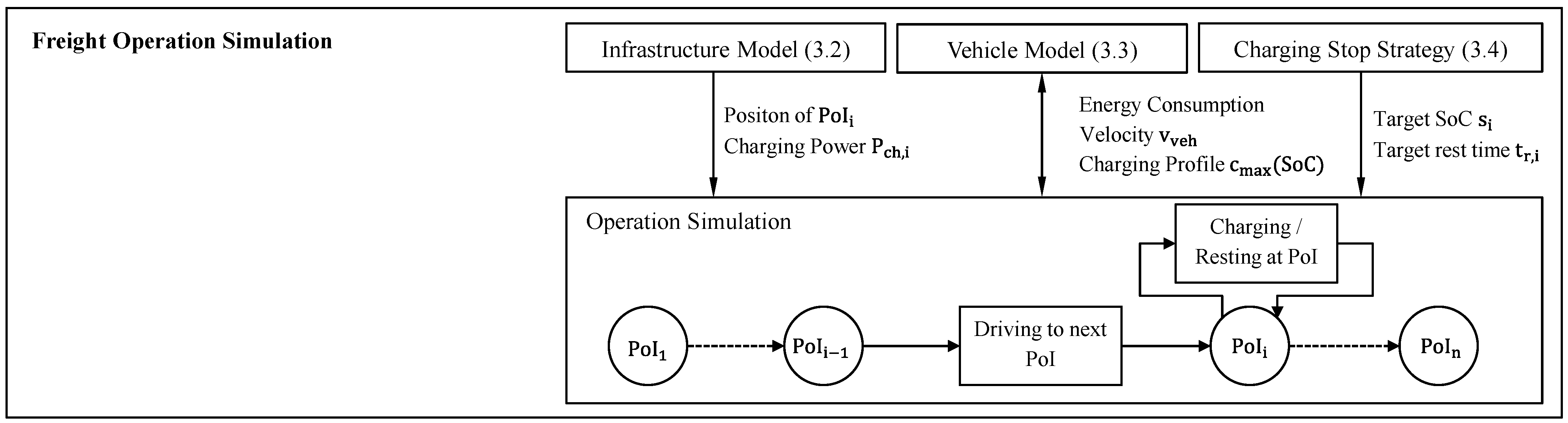
The simulation environment includes the operation simulation, the necessary infrastructure, and vehicle model, as well as the mentioned charging stop strategies (Figure 2).
The operation simulation is carried out in a PoI-based manner. We define PoIs here as rest sites both with and without charging possibility. Analogous to Huber et al. [18,26] and Cussigh et al. [27], we assume a defined route, which is described by the total distance and a constant average velocity. Along the defined route, the PoIs are set through the infrastructure model. The trip between two PoIs is simulated using the vehicle model, which incorporates the vehicle energy consumption and the travel time by the average velocity. The action at a PoI is controlled by the charging stop strategy. This specifies the rest time and target SoC level at . The vehicle is charged until the desired SoC level . If the desired rest time has not yet been reached by the charging event, the remaining time is added. The used vehicle and infrastructure model are shown in more detail below.
3.2. Infrastructure Model
Since no dedicated charging infrastructure for BET has been installed so far, we show a synthetically modeled infrastructure that depicts rest areas with and without charging possibilities. For this purpose, equidistant PoI positions are assumed along the defined route, which are spaced at intervals of , based on the guideline for rest sites on German highways [28]. Not every PoI offers a charging possibility. The positions of the charging points are controlled by the resolution. For a reference scenario, a resolution is assumed [29] so that every second PoI offers a charging point. This assumes that charging points for BET are initially set up at managed rest areas that can be found at intervals of 50 to 60 km on German highways [28]. Each charging point is equipped with the charging power . The modelling of the charging infrastructure is static. Therefore, the properties are constant in time. We assume that the charging points are always available. For the driving simulation, a vehicle model is further required.
3.3. Vehicle Model
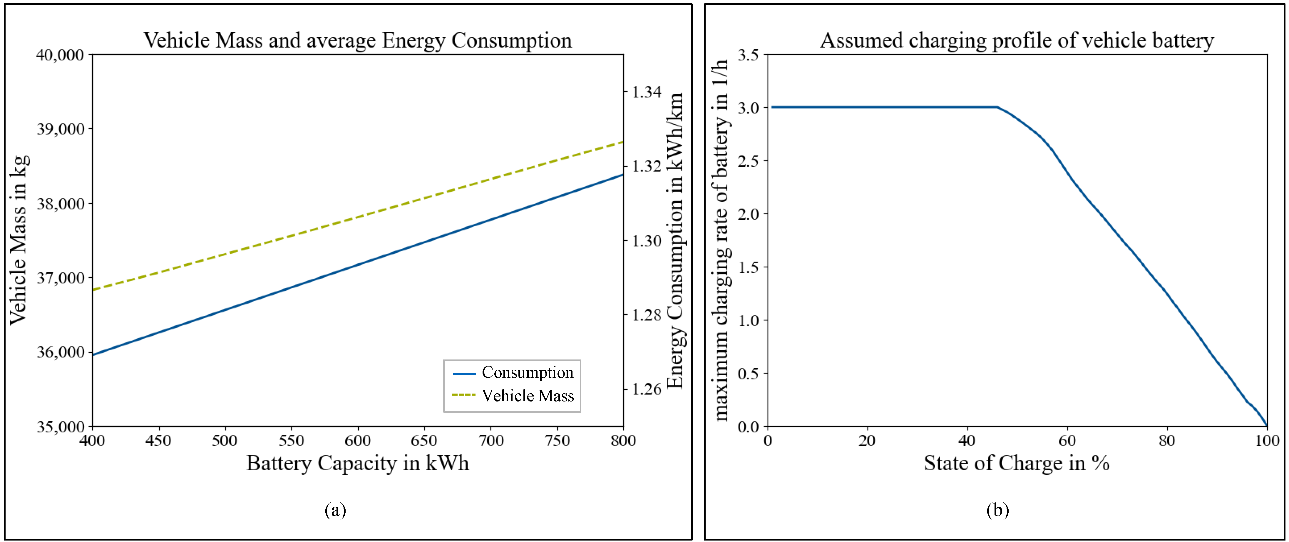
The vehicle model used for the potential analysis must be able to represent the driving interval between two PoIs as well as the necessary charging cycles. Therefore, we used a constant energy consumption and vehicle velocity for the driving simulation. It must be considered that the consumption depends on the vehicle mass and thus crucially on the battery capacity (Figure 3a).
The consumption values used in this paper are the result of an energy consumption simulation based on the VECTO Long Haul cycle [31]. This simulation is constructed as a forward simulation and includes a detailed powertrain model. The basics of the implementation of this simulation can be taken from Appendix A. In the further calculations, the values from Figure 3a are used to keep the simulation time low.
In addition to the driving sections, possible charging events must be considered. For this purpose, a battery model is used that is described by the possible charging rate as a function of the State of Charge (SoC). According to charging power benchmarks presented by Daake et al. [32], we assume a maximum charging rate , which degrades at a higher SoC (Figure 3b) [30]. For this, the conventional constant current constant voltage (CCCV) charging protocol is assumed. Charging is performed at the defined maximum charging rate until the maximum cell voltage is reached. The charging rate is then reduced so that the maximum voltage is constant [33]. The operation simulation with the described models will be used to show the potential of an optimal charging stop strategy (FO) compared to a simple “Not Getting Stranded” strategy (NGS).
3.4. Charging Stop Strategies
To enable comparability of both considered strategies, they were subject to certain boundary conditions. Assuming overnight charging at private sites, a journey begins with a fully charged battery . When reaching the final destination, a SoC of must be ensured as a safety factor. In addition, both strategies must comply with the mandatory rest schedules. Accordingly, after a driving time of a rest of at least must be taken. Within the driving interval, the rest can also be divided into a 15 and 30 min sequence [13]. For the potential estimation of an optimal charging stop strategy, the assumed decision chosen by the driver without full information should be first formulated in the NGS strategy as a reference.
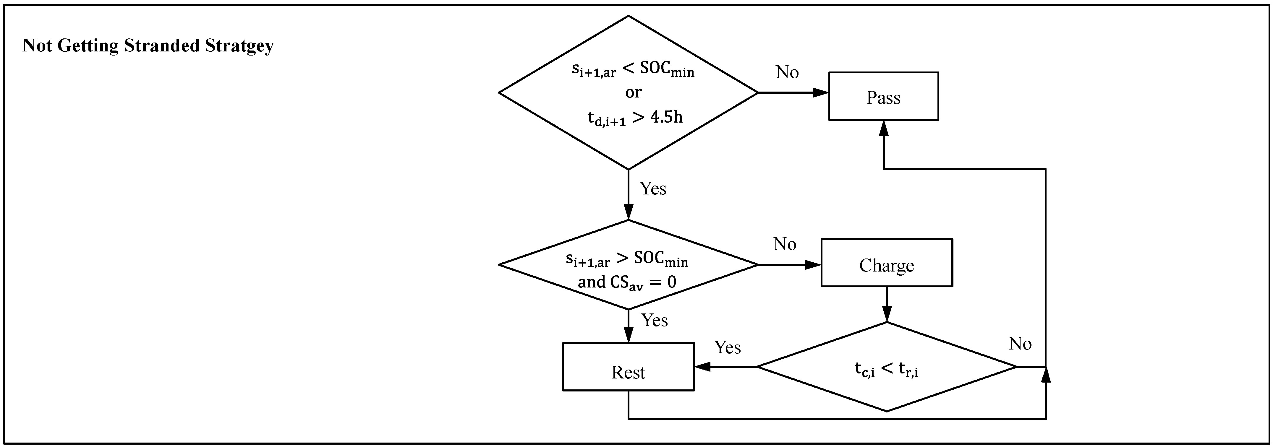
3.4.1. Not Getting Stranded Strategy
The NGS strategy is limited only to the driver’s knowledge of the range and locations of charging stations on the route. In addition, it is assumed that the driver can estimate the travel time between two PoIs based on his experience. Based on this, we assume that the driver will act according to the following rules:
- The driver takes the full mandatory rest at the upcoming PoI if the driving time to the next PoI exceeds his permitted driving time .
- The vehicle is charged at the upcoming PoI with a charging point if the range is less than the distance to next charging station on the route.
The driver’s action can thus be formulated as a strategy by the decision tree shown below (Figure 4). The NGS strategy, which serves as a reference, is challenged by the FO strategy that is shown in the next section.
3.4.2. Fully Optimized Strategy
The FO strategy represents the solution of an optimization problem. This is descried mathematically in the following. The decision variables are the rest time at the relevant as well as the SoC level when leaving a with a charging possibility. Therefore, the decision vector consists of the two components and .
In the rest times are located at the relevant PoI. To keep the number of decision variables small, only the PoIs are considered that can be reached within a pure travel time of to comply with the mandatory rest schedules. Only these PoIs are considered for an optimal located rest.
The possible entries in are defined as discrete integer variables. The integer values are assigned to a rest period of 0, 15, 30, and 45 min. Due to the mandatory rest schedules to be observed, this simplification can be made without restricting the optimal solution.
At the SoC level when leaving the with a charging opportunity is located. Therefore, the entries in are continuous. With a charging infrastructure resolution , the length of corresponds to the number of the PoI along the route.
The optimization objective addresses the integrability into existing logistic processes and is consequently selected as the duration of the considered entire freight mission. This results from the pure driving time and the time required for charging and rest .
For constant speed between two PoIs, , the travel time of the route is calculated as follows.
The total duration of the charging and rest operations result as the sum of the individual actions.
The duration for a charging or rest operation of a corresponding PoI, , is calculated based on the arrival SoC and the entries of the decision vector.
The pure charging time is calculated based on the current SoC level, , and the SoC-dependent charging rate, . The used charging rate is the minimum from the maximum possible rate, (Figure 3b), and the resulting charging rate from the charging power available at the charging point. The SoC level is discretized in one percent steps, .
For the charging process, a connection time of is considered [27]. This includes the time lost by leaving the highway, connecting, billing, and re-entering the highway.
The rest time is calculated considering the charging time and the entry in the decision vector at the current PoI.
If the rest stop is connected to a charging process at the same PoI, the leaving and re-entering onto the highway was already considered. If a pure rest stop is completed , a time is considered.
This sufficiently describes the objective function based on the decision vector. The compliance with the rest schedules is achieved by two unbalanced constrains. After a driving time of , a total rest period of 45 min must be completed.
Furthermore, rest split is allowed if one of the two splits is at least 30 min.
In summary, the optimization problem at hand can be described as follows.
The limits of represent physically reasonable SoC limits.
The optimization problem is classified as a mixed-integer, non-linear problem (MINLP) due to the split between discrete and continuous entries in the decision vectors and the non-linear charging behavior. For solving optimization problems, there are three main methodologies possible [34]. Enumerative methods are not suitable for continuous variables, since there are an infinite number of possibilities. In addition, the computational effort for a full factorial calculation is very high for a large number of PoIs. Deterministic methods are unsuitable for discontinuous problems [34]. Therefore, we chose a stochastic method for the solution of the formulated optimization problem.
The genetic algorithm, as one of the stochastic methods, has proven to be suitable for solving technical problems, which is why it will be used here [5]. For this purpose, the open-source Python library Pymoo [35] and the single-objective genetic algorithm available therein were used. The optimization was performed with the number of individuals , which was adapted to the number of entries, , in the design vector . The coupling is necessary to guarantee the same properties of the solution algorithm for a varying number of PoIs (Section 4). It has been shown that for this number of individuals a generation number of 100 leads to convergence of the solution algorithm.
It should be mentioned again that static infrastructure properties were assumed; thus, the global optimal strategy for the entire route can be determined before the freight mission starts by solving the optimization problem shown before. These strategies are applied to a freight scenario in the driving simulation shown in the following section and thus allow the potential estimation of the FO strategy in comparison to the NGS strategy.
4. Application and Results
Long-haul applications are considered difficult to electrify due the high daily milage. However, this also offers the highest saving potential for CO2 emissions. We therefore consider such a scenario with an assumed trip length of 700 km. Further, we assume a constant speed of 82 km/h, which corresponds to the average speed of the VECTO LH cycle [31]. This speed results in a pure travel time of , which is close to the daily allowed driving time of 9 h. Along this distance, the infrastructure model defines the PoI. Every 25 km there is a rest site, resulting in a total of 28 PoIs. As a baseline, the charging infrastructure resolution is set to , corresponding with the target set by the German federal government [29]. It is assumed that all charging stations supply the same power of . For this setting, the potential of the FO strategy is shown in the next section for answering the first two research question we identified in the beginning.
4.1. Potential Estimation of FO Strategy
We chose the time loss, , that is expected using BET for the potential analysis and thus address the integrability of BET into existing logistic processes. The time loss is determined in relation to the trip with an ICET. The total time for the trip with ICET corresponds the pure driving time added with the time for leaving and re-entering the highway for one mandatory stop and the necessary rest time .
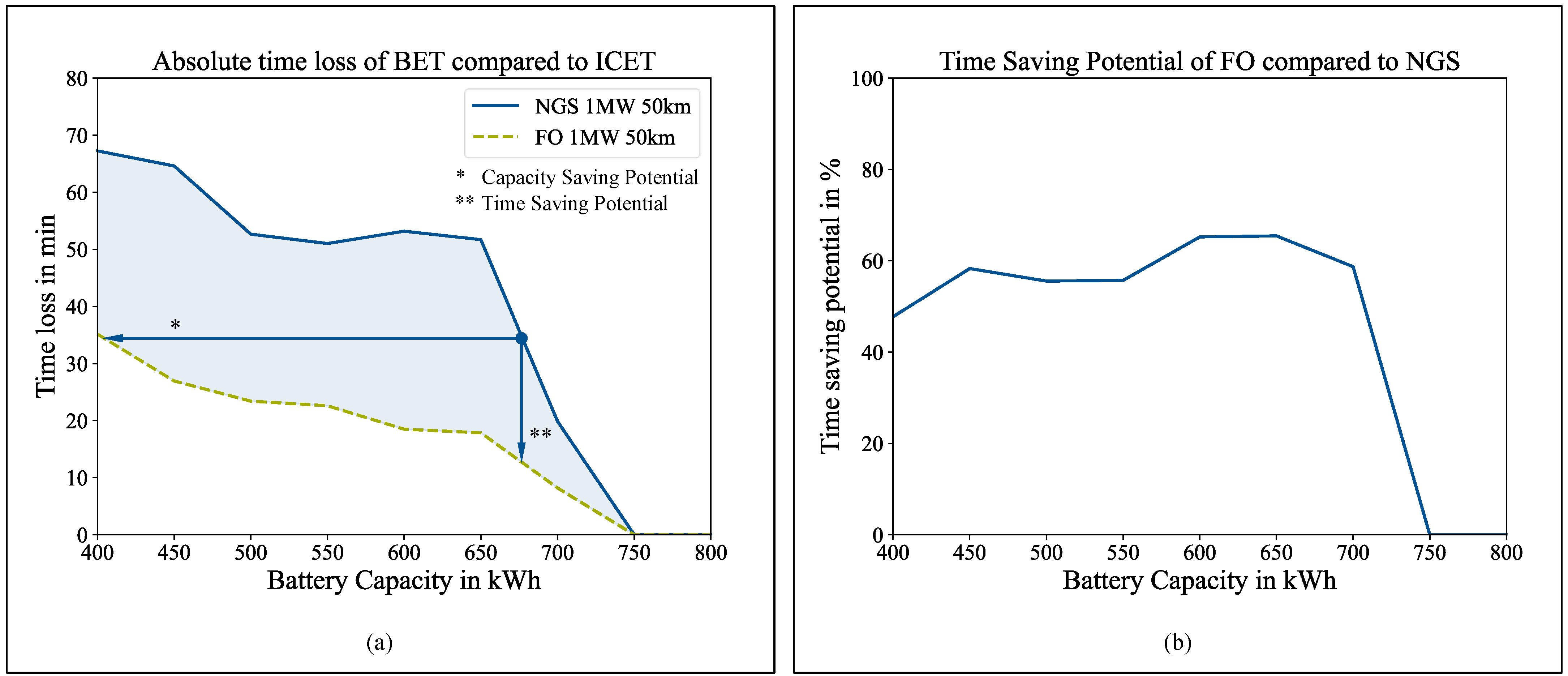
Besides the time loss, the investment cost is a hurdle that is directly proportional to the battery capacity of the BET. Therefore, Figure 5a shows the expected time loss for the NGS and FO strategy over the installed battery capacity of the BET. On the right-hand side (Figure 5b), the relative time-saving potential of the optimized strategy (FO) compared to the NGS strategy is presented.
The potential of an optimal charging stop strategy can interpreted as the area between the two curves. If the battery capacity is kept constant, this results in the time-saving potential (**), while if the time loss is accepted, the battery can be reduced with an optimal strategy (*) and consequently the investment costs can be significantly reduced.
The results show that up to a battery capacity of , a time loss must be expected in any case if a charging power of is available. For lower battery capacities, the time loss can be reduced by at least 50% through an optimal strategy over a wide range of battery capacities. For battery capacities smaller than 675 kWh, the results show that with an optimal strategy (FO) already a capacity of 400 kWh results in significantly lower time loss than without a strategy (NGS). Therefore, a capacity-saving potential of 275 kWh can be achieved by using an optimal charging stop strategy. Building on these results, in the next section we aim to answer the third research question of what impact charging infrastructure properties have on time loss and which strategy is more sensitive to such changes.
4.2. Influence of Infrastructure Properties
The two key properties of the static infrastructure model are the available charging power, , and resolution, , of the charging points along the route. For these two properties a variation is performed.
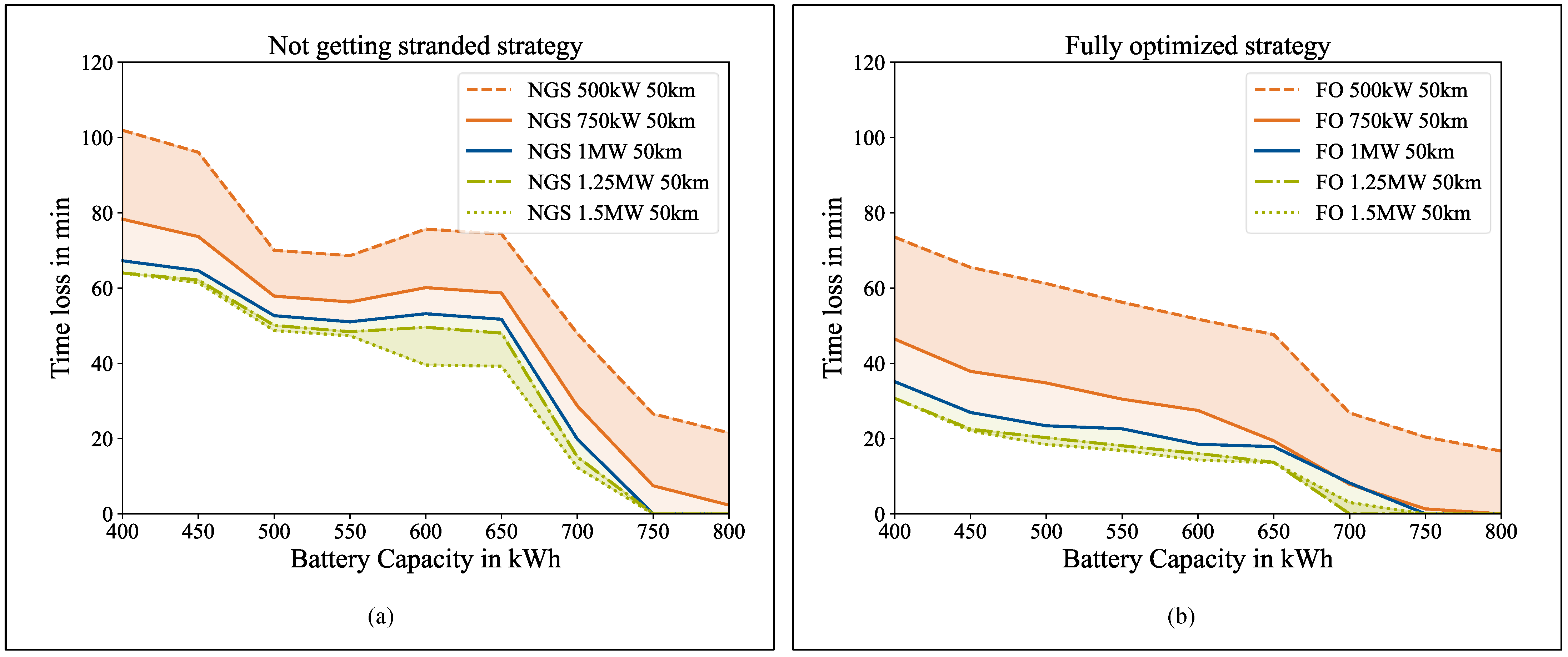
We continue to consider only static properties that do not change during the trip. Furthermore, the charging power is kept the same at all charging sites. The position of these remains equidistant. Figure 6 shows the effect of changing the charging power on the expected time loss for both strategies. The distance between the charging points is still 50 km .
Based on the setting considered so far (blue), a reduction in the available charging power to for both strategies results in a small increase in time loss. The FO strategy can compensate for this reduction for high battery capacities. However, if the charging power is even lower , a significantly higher time loss is to be expected for both strategies. It is also shown that the optimal strategy (FO) reacts more sensitively to the power reduction. Yet, it outperforms the NGS strategy at all times.
An increase in the power to is expected to be beneficial across the entire battery capacity range, with the FO strategy leading to slightly higher saving potential. The further increase to 1.5 MW, on the other hand, seems less profitable. For battery capacities below 500 kWh, the charging rate of (Figure 3b) is limiting here. However, even for higher battery capacities, such a high charging power leads only to minimal improvement.
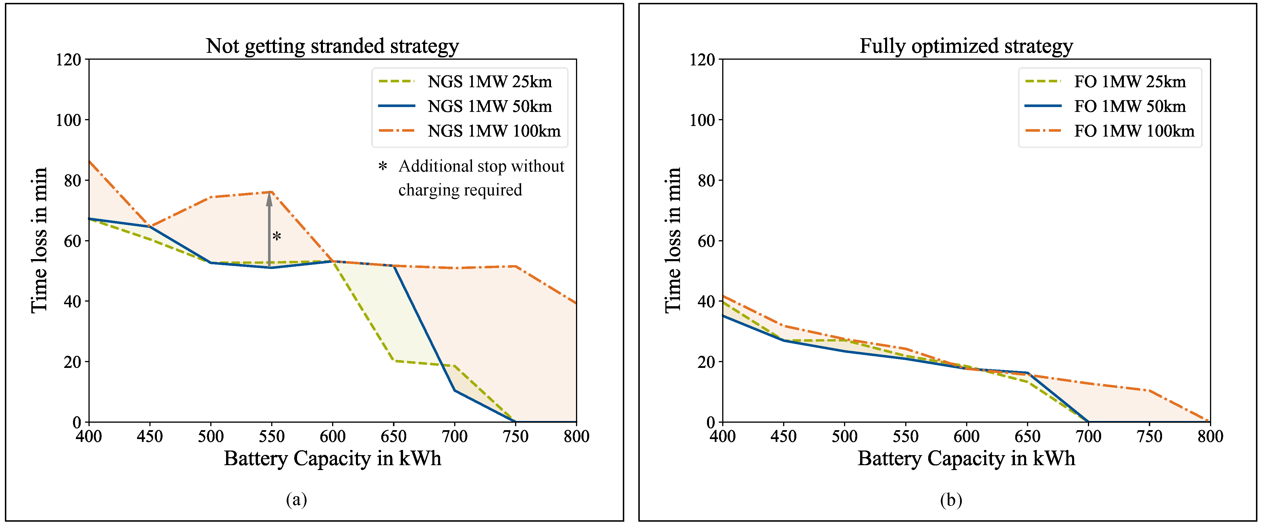
Overall, it is clearly shown that the optimal strategy and a charging power of 1 MW at a minimum can reduce the time loss to less than 20 min for a wide range of battery capacities. However, it is highlighted that low power cannot be fully compensated for by an optimal strategy. This leads to the conclusion that a charging power above 1 MW for on route charging is mandatory for a low time loss. The second influencing factor to be analyzed is the resolution of the charging sites, . This is shown in Figure 7 It should be noted that the availability of the charging sites is still given at all times. The charging power corresponds to the initial setting ().
For the NGS strategy, a clear dependence on the infrastructure resolution is shown (Figure 7a). A higher resolution of 25 km shows less advantages whereas the reduced resolution of 100 km shows significantly higher time loss for many battery capacities. This increase in time loss is the result of additional stops at rest sites without charging possibility due to the mandatory rest times after 4.5 h of driving. For a range of battery capacities there is no dependence on the infrastructure resolution. This can be explained by the fact that the charging stops take place at those charging stations that are available for all resolutions. In contrast to the NGS strategy, there is hardly any effect for the FO strategy at both an increased and reduced resolution (Figure 7b). Only for high battery capacities at a resolution of 100 km a time loss is to be expected, which would not occur with a higher resolution.
Figure 7.
Influence of infrastructure resolution (distance between two charging sites) on absolute time loss using (a) the NGS strategy and (b) FO strategy. In contrast to NGS, the FO strategy can compensate for a sparse infrastructure resolution for most battery capacities.
Figure 7.
Influence of infrastructure resolution (distance between two charging sites) on absolute time loss using (a) the NGS strategy and (b) FO strategy. In contrast to NGS, the FO strategy can compensate for a sparse infrastructure resolution for most battery capacities.

In summary, when using optimal strategies, the influence of the charging power is to be rated significantly higher than the local resolution of the charging sites, if these are available in sufficient quantity. For the assumptions on which this is based, a charging power of at least 1 MW should be aimed to keep the time loss low. In the following, we close with a discussion and brief outlook.
5. Discussion
We have shown the potential of an optimal charging stop strategy in the previous section. This can be interpreted both in terms of time and in the context of investment costs via the battery capacity. The investigations show that especially for low and medium battery capacities there is a very high potential for reducing the time loss, but that even with an optimal strategy a time loss must be expected. The concrete value to which a time loss is acceptable depends on the underlying freight mission and, thus, on the freight forwarder. An increase in the charging power only provides a limited remedy. Further investigations should be carried out to determine if an even higher charging power and capable battery cells bring advantages here. In the results presented here, cells were charged to a maximum of 3 C (Figure 3b). Another reason is the driving regulations [13] that apply in Europe. If the driving section after the 45-min rest cannot be driven without charging, a time loss occurs. A higher charging power can therefore only eliminate the time loss on combination with less driving regulation and thus resolve the trade-off between time and battery capacity.
The potential estimation was based on a complete modeling of the infrastructure, whose parameters are based on assumptions. Currently, there is no dedicated charging infrastructure for BET; so, real mapping is impossible. The resolution of the rest sites on German highways was used here [28]. The authors consider it likely that initially the managed rest sites will be equipped with charging infrastructure for BET. However, it is uncertain in which power ranges the charging stations will be available. We have assumed a constant power across all charging power points; this picture is unlikely to be seen in reality. Further research can show the impact of varying charging power across charging points. In addition, we only modeled the public charging infrastructure for performing the charging events. However, BET could also be charged at private logistic sites. The assumption of equidistant positions of the PoIs then seems not applicable. Such considerations will be carried out in future work. Another simplification is the purely static modelling approach. This concerns both the vehicle and the infrastructure side. On the vehicle side, we assume a constant energy consumption that depends only on battery capacity. Dynamic events, resulting in locally higher energy consumption, have complex SoC predictions, and require a dynamically adaptive strategy while driving. Analogous considerations apply to the prediction of arrival times by a constant speed over the trip. On the infrastructure side, we assumed that charging points are always available. Considering that dynamic occupancy probabilities and varying charging power significantly increase the complexity of infrastructure modeling, online-capable charging strategy planning is required. For the results shown, we used a global optimization approach to set the strategy before the trips starts. Furthermore, the simplification remains that a fixed route is not changed during the trip by the dispatcher or navigation system. This restriction seems justifiable, since fast-charging points are initially set up along the motorways, so that rerouting is initially difficult due to the lack of charging stations.
From a methodological point of view, we have chosen a stochastic approach for solving the optimization problem. Due to the coupling of two decision variables per PoI, one of which was chosen as discrete, discontinuities are to be expected, so that this solution method was considered suitable here [34]. Previous, mostly graph-based methods, shown in the literature lead, to large graphs due to this coupled decision variables, and therefore are rated as unsuitable. However, it remains unclear whether other stochastic methods provide an advantage over the genetic algorithm used. Knowing the limitations of equidistant PoIs, constant charging power, and purely static vehicle and infrastructure properties, as well as global strategy optimization before driving, we want to motivate the research field of charging stop strategies for BET and encourage others to perform more realistic investigations. We close this paper with a brief conclusion and outlook.
6. Conclusions and Outlook
Electrification is essential for the decarbonization of road freight transport. BET offer great potential here due to their high well-to-wheel efficiency. For a fast transformation, it is necessary to satisfy all stakeholders of BET. This includes not only the hauler but also the drivers. The optimal integration of charging stops into the operation while complying with the mandatory rest schedule requires a high level of information and its processing. Managing this task on top seems very difficult, which is why driver support is necessary here. Moreover, it is still unclear to what extent the BET can be integrated into existing logistic process and what time losses are to be expected for the necessary charging cycles.
Based on this, we have shown for the first time the potential of an optimal charging stop strategy for BET. For this purpose, the infrastructure properties remain static. We have shown that an optimal strategy can greatly reduce the expected time loss, for energy capacities already available today, which is less than 20 min for a trip duration more than 8 h. This requires an available charging power of at least 1 MW, which will be given by the new MCS standardization and current research projects [10,36]. It has been shown that especially for a reduced power of only 500 kW, the time loss for long-haul applications increases significantly. This motivates the initial installation of the charging points above 1 MW of power to make transformation to BET manageable for truck drivers. For optimal strategies, the resolution of the charging points does not play a significant role. This is under the assumption that the charging points are always available and thus in sufficient numbers installed. From an investment point of view, it can be more favorable to have fewer charging parks with more charging points due the grid connection. However, the high peak load of the local electricity could be a disadvantage.
In future work, a step towards situational dynamic charging stop strategies will be shown. In addition to the time aspect, we want to illuminate the cost side and integrate the possibility of depot and public charging into charging stop strategies, too.
Author Contributions
First author, M.Z.; conceptualization, M.Z. and J.S.; methodology, M.Z., S.W. and J.S.; software, M.Z. and J.S.; validation, M.Z., J.S. and S.W.; formal analysis, S.W., J.S. and G.B.; investigation, M.Z.; data curation, J.S. and G.B.; writing—original draft preparation, M.Z.; writing—review and editing, S.W. and J.S. and G.B.; visualization, M.Z.; supervision, M.L.; funding acquisition, S.W. All authors have read and agreed to the published version of the manuscript.
Funding
The research of M.Z., J.S.; and G.B. was funded by Federal Ministry for Economic Affairs and Climate Protection within the research project NEFTON (FKZ: 01MV21004A). The research of S.W. was conducted with the basic research funds from the Institute of Automotive Technology, Technical University of Munich.
Acknowledgments
M.L. gave final approval of the version to be published and agrees to all aspects of the work. As a guarantor, he accepts responsibility for the overall integrity of the paper.
Conflicts of Interest
The authors declare no conflict of interest.
Appendix A
Appendix A.1. Driving Simulation for Energy Consumption Estimation
The consumption values used for the shown potential estimation of an optimal charging stop strategy were taken from an energy consumption simulation, which will be presented here. For this, we first show the driving simulation and afterwards the used powertrain model for this. All parameters used can be found in (Appendix A.3.)
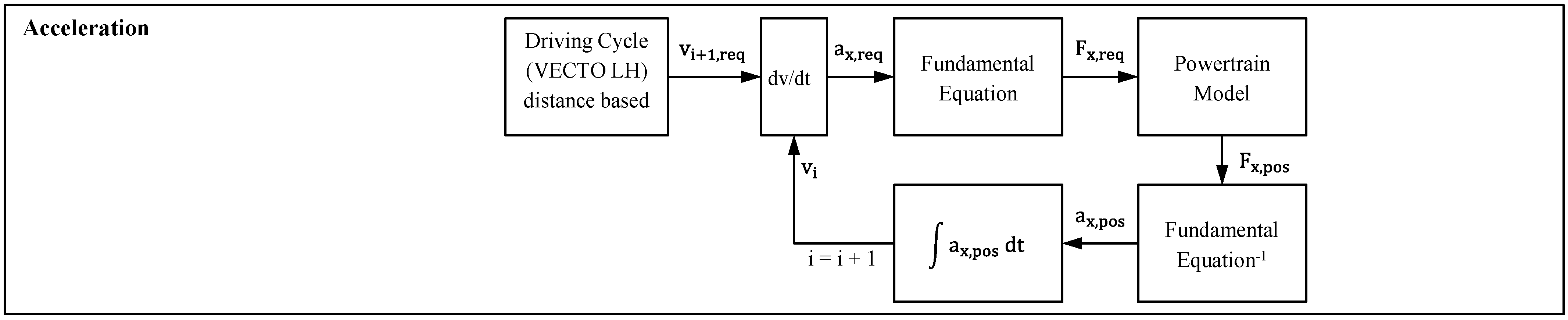
The driving simulation is distance-based with a resolution of one meter. In each distance step, a target acceleration is calculated based on the current vehicle velocity and the specified driving cycle velocity. In contrast to the common BEV energy consumption simulation, such as in [37], a pure backward simulation cannot be used for commercial vehicles. In most cases, the truck does not reach the prescribed acceleration of the driving cycle, so that the driven cycle deviates from the prescribes one. Therefore, a backward simulation is combined with a forward simulation in this work. For the acceleration case , the vehicle velocity in the next distance step is calculated according to the scheme shown below (Figure A1).
Figure A1.
Simulation step of the detailed driving simulation in case of acceleration.

The required acceleration, , is calculated based on the current vehicle velocity, , and the prescribed velocity in the next distance step,
Based on the fundamental equation of vehicle dynamics, the required tractive force at the wheelbase, , is calculated. The force requirement is the input for the powertrain model, which we show below (Appendix A.2.). In each component of the powertrain, it is determined whether the force, resulting torque, or power can be provided or must be reduced. The result of the powertrain model is the providable force at the wheelbase, From this, the acceleration achieved and the resulting velocity in the next distance step can be calculated. Since no driver model is considered here, it is assumed that the vehicle tries to follow the given cycle with maximum possible acceleration.
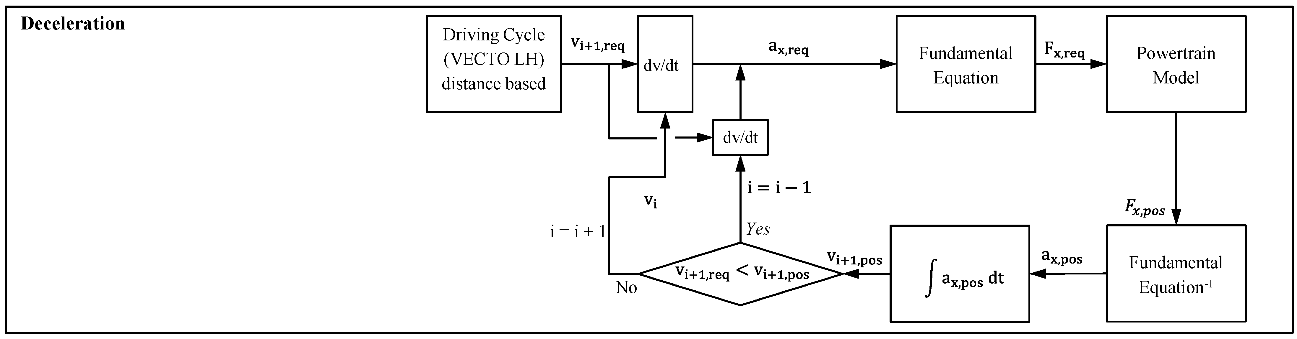
In case of deceleration , the calculation of the velocity in the next distance step follows the scheme in Figure A2.
Figure A2.
Simulation step of the detailed driving simulation in case of deceleration.

Analogous to the acceleration step, for deceleration, the required tractive force ( is calculated. As a result of the powertrain simulation, the possible tractive force and resulting deceleration is carried out, considering the recuperation capability and the maximum brake force. The velocity in the next distance step results from the deceleration. If the achieved speed is the one prescribed, the next distance step can be simulated. However, if the desired deceleration cannot not be achieved, the current distance step (brake point) is shifted back by one step. This corresponds to braking earlier. The brake point is therefore reset until the speed in the target distance step can be reached. In summary, the forward simulation checks whether the acceleration values can be achieved by the powertrain and whether the brake point is set in such a way that the target speed can be reached. Through this driving simulation, we calculate the energy consumption for one VECTO LH cycle [31], which we use for the shown potential analysis. In the next two sections, we present the mentioned powertrain model and the used parametrization.
Appendix A.2. Powertrain Modeling Approach for the Energy Consumption Simulation
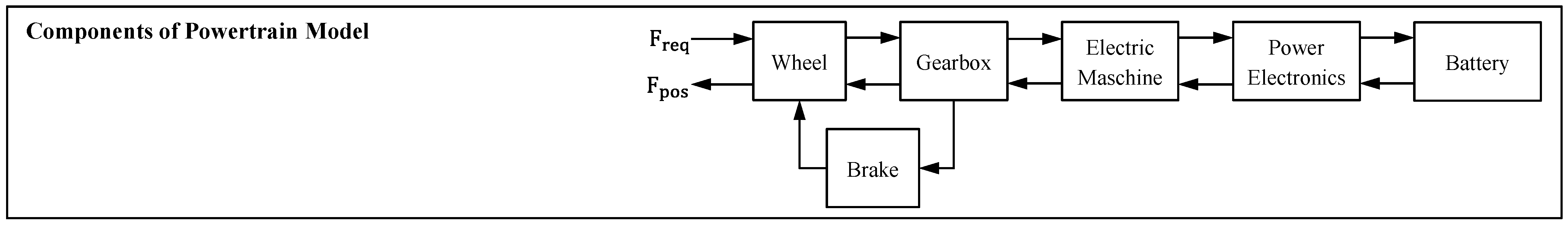
The powertrain model has as input parameters the required tractive force at the wheelbase from the fundamental dynamic equations, such as air resistance force, and provides as output the possible tractive force that the individual components of the powertrain can provide. For this, the model includes the gearbox, brake, electric machine, power electronics, and the battery (Figure A3).
Figure A3.
Components of the suggested powertrain model for energy consumption estimation.

Based on the required tractive force at the wheelbase, the required torque is calculated via the dynamic wheel radius. The transmission model considers the gear ratio, , and a constant efficiency, .
Based on that, the efficiency of the electric machine is determined via interpolation within an efficiency map provided by [38] on the basis of torque and speed .
In case of deceleration, a recuperation rate, , is considered. Since only the rear axle can be braked via recuperation, driving dynamic instabilities can occur if the recuperation torque is too high. Therefore, a recuperation rate of 50% is applied from a deceleration onwards, For a lower deceleration, we assume . If the required torque, , exceeds the maximum torque of the electric machine, , the machine torque is passed on. The required power, , of the machine represents the power request to the battery model, , by consideration of the efficiency, , of the power electronics. Together with the time required for a distance step , the required power are the input variables in the battery model. The time duration, , is calculated based on the current vehicle speed and the required acceleration .
The required energy, , for driving distance step with acceleration can be calculated from the required power, , added by the auxiliary consumption , and the time step . The battery modelling for the driving simulation was carried out according to Schmalstieg et al. [39] and therefore not described further here.
The battery model provides as output the power , which the battery can provide based on its current state. Based on this, the powertrain model blocks the power electronics electric machine and the gearbox runs inversely according to the shown relationships. In case of deceleration, the wheel brake can provide additional torque for recuperation. The brake force is added to the force from recuperation at the wheelbase.
We assume a maximum braking force of This value results from the permissible axle load of the tractor with full utilization of a friction coefficient of one. If the required additional brake force is greater, the maximum brake force is applied. The possible tractive force at the wheelbase results from the output of the powertrain model. From this, the possible acceleration, , is further calculated. If this value deviates from the required acceleration, or if a component has reduced its request, the acceleration specification is replaced with and the powertrain model is run through again. The parametrization of the vehicle model and the mass modeling can be found below (Appendix A.3.).
Appendix A.3. Used Vehicle Data and Parameters

Table A1.
Vehicle dynamics and powertrain parameters. The bold parameters are used in final simulation.
Table A1.
Vehicle dynamics and powertrain parameters. The bold parameters are used in final simulation.
| Parameter | Abbreviation | Value | Source |
|---|---|---|---|
| Drag coefficient | 0.6, 0.55 | [40,41] | |
| Frontal Area | [40] | ||
| Density Air | [40] | ||
| Gravimetric Acceleration | g | - | |
| Rolling resistance coefficient | 0.0055, 0.005 | [40,41] | |
| Dynamic Tire Radius | 0.4465 m | [38] | |
| Electric machine efficiency map | [38] | ||
| Electric machine max torque | 2018 Nm | [38] | |
| Auxiliaries Consumers | 4 kW | [41] |
Table A2.
Mass of vehicle components.
| Weight Parameter | Abbreviation | Value | Source |
|---|---|---|---|
| Trailer Mass | 7500 kg | [42] | |
| Tractor without powertrain | 5400 kg | [42] | |
| Payload | 19.300 kg | [31] | |
| Density Electric Machine | 0.5 kg/kW | [43] | |
| Density gearbox | kg/Nm | [44] | |
| Density Powerelectronics | 0.078 kg/kW | [43] | |
| Gravimetric Density Battery Pack | 165 Wh/kg | [45] |
References
- Statista, CO2-Ausstoß Weltweit Nach Sektoren | Statista. Available online: https://de.statista.com/statistik/daten/studie/167957/umfrage/verteilung-der-co-emissionen-weltweit-nach-bereich/ (accessed on 19 July 2022).
- European Commission. Directorate General for Mobility and Transport, EU Transport in Figures: Statistical Pocketbook 2021; Publications Office: Luxembourg, 2021. [Google Scholar]
- Umweltbundesamt, CO2-Gesetzgebung: Flottenzielwerte für Schwere Nutzfahrzeuge. Available online: https://www.umweltbundesamt.de/themen/verkehr-laerm/emissionsstandards/schwere-nutzfahrzeuge (accessed on 18 March 2022).
- Wolff, S.; Fries, M.; Lienkamp, M. Technoecological analysis of energy carriers for long-haul transportation. J. Ind. Ecol. 2020, 24, 165–177. [Google Scholar] [CrossRef]
- Wolff, S.; Seidenfus, M.; Brönner, M.; Lienkamp, M. Multi-disciplinary design optimization of life cycle eco-efficiency for heavy-duty vehicles using a genetic algorithm. J. Clean. Prod. 2021, 318, 128505. [Google Scholar] [CrossRef]
- Plötz, P. Hydrogen technology is unlikely to play a major role in sustainable road transport. Nat. Electron. 2022, 5, 8–10. [Google Scholar] [CrossRef]
- Transport and Environment. Comparison of Hydrogen and Battery Electric Trucks: Methodology and Underlying Assumptions. Available online: https://www.transportenvironment.org/discover/comparing-hydrogen-and-battery-electric-trucks/ (accessed on 10 September 2022).
- Mao, S.; Basma, H.; Ragon, P.; Zhou, Y.; Rodriguez, F. Total Cost of Ownership for Heavy Trucks in China: Battery Electric, Fuel Cell, and Diesel Trucks. Available online: https://theicct.org/publication/total-cost-of-ownership-for-heavy-trucks-in-china-battery-electric-fuel-cell-and-diesel-trucks/ (accessed on 9 September 2022).
- Hunter, C.; Penev, M.; Reznicek, E.; Lustbader, J.; Birky, A.; Zhang, C. Spatial and Temporal Analysis of the Total Cost of Ownership for Class 8 Tractors and Class 4 Parcel Delivery Trucks; Technical Report; National Renewable Energy Laboratory: Golden, CO, USA, 2021. [Google Scholar]
- CHARIN, Megawatt Charging System (MCS). Available online: https://www.charin.global/technology/mcs/ (accessed on 27 April 2022).
- electrive.net, NEFTON: Entwicklung von E-Lkw und Megawatt-Ladegerät—Electrive.net. Available online: https://www.electrive.net/2021/10/19/nefton-entwicklung-von-e-lkw-und-megawatt-ladegeraet/ (accessed on 14 April 2022).
- Mareev, I.; Becker, J.; Sauer, D. Battery Dimensioning and Life Cycle Costs Analysis for a Heavy-Duty Truck Considering the Requirements of Long-Haul Transportation. Energies 2018, 11, 3446. [Google Scholar] [CrossRef]
- Bundesamt für Güterverkehr, Fahrpersonalrecht. Available online: https://www.bag.bund.de/DE/Themen/RechtsentwicklungRechtsvorschriften/Rechtsvorschriften/Fahrpersonalrecht/fahrpersonalrecht_node.html (accessed on 26 April 2022).
- Williams, D.F.; Thomas, S.P.; Liao-Troth, S. The Truck Driver Experience: Identifying Psychological Stressors from the Voice of the Driver. Transp. J. 2017, 56, 54–76. [Google Scholar] [CrossRef]
- Transport Logistic, LKW-Fahrermangel: Fachkräftemangel in der Logistik Lösen. Available online: https://transportlogistic.de/de/messe/industry-insights/lkw-fahrermangel/ (accessed on 18 March 2022).
- Flood, M. The Traveling-Salesman Problem. Oper. Res. 1956, 4, 61–75. [Google Scholar] [CrossRef]
- Kobayashi, Y.; Kiyama, N.; Aoshima, H.; Kashiyama, M. A route search method for electric vehicles in consideration of range and locations of charging stations. In Proceedings of the 2011 IEEE Intelligent Vehicles Symposium, Baden-Baden, Germany, 5–9 June 2011; pp. 920–925. [Google Scholar]
- Huber, G.; Bogenberger, K. Long-Trip Optimization of Charging Strategies for Battery Electric Vehicles. Transp. Res. Rec. 2015, 2497, 45–53. [Google Scholar] [CrossRef]
- Sweda, T.M.; Klabjan, D. Finding minimum-cost paths for electric vehicles. In Proceedings of the 2012 IEEE International Electric Vehicle Conference, Greenville, SC, USA, 4–8 March 2012; pp. 1–4. [Google Scholar]
- Erdelić, T.; Carić, T. A Survey on the Electric Vehicle Routing Problem: Variants and Solution Approaches. J. Adv. Transp. 2019, 2019, 1–48. [Google Scholar] [CrossRef]
- Dijkstra, W.E. A Note on Two Problems in Connexion with Graphs. Numer. Math. 1959, 1, 269–271. [Google Scholar] [CrossRef]
- Artmeier, A.; Haselmayr, J.; Leucker, M.; Sachenbacher, M. The Shortest Path Problem Revisited: Optimal Routing for Electric Vehicles. In KI 2010: Advandces in Artificial Intelligence; Dillman, R., Beyerer, J., Hanebeck, U.D., Schultz, T., Eds.; Lecture Notes in Computer Science; Springer: Berlin/Heidelberg, Germany, 2010; Volume 6359. [Google Scholar]
- Storandt, S.; Stefan, F. Cruising with a Battery-Powered Vehicle and Not Getting Stranded. In Proceedings of the Twenty-Sixth AAAI Conference on Artificial Intelligence, Toronto, ON, Canada, 22–26 July 2012. [Google Scholar]
- Pourazarm, S.; Cassandras, C.G. Optimal routing of energy-aware vehicles in networks with inhomogeneous charging nodes. In Proceedings of the 22nd Mediterranean Conference of Control and Automation (MED 2014), Palermo, Italy, 16–19 June 2014. [Google Scholar]
- Schneider, M.; Stenger, A.; Goeke, D. The Electric Vehicle-Routing Problem with Time Windows and Recharging Stations. Transp. Sci. 2014, 48, 500–520. [Google Scholar] [CrossRef] [Green Version]
- Huber, G.; Bogenberger, K.; van Lint, H. Optimization of Charging Strategies for Battery Electric Vehicles Under Uncertainty. IEEE Trans. Intell. Transport. Syst. 2022, 23, 760–776. [Google Scholar] [CrossRef]
- Cussigh, M.; Hamacher, T. Optimal Charging and Driving Strategies for Battery Electric Vehicles on Long Distance Trips: A Dynamic Programming Approach. In Proceedings of the IV19: 30th IEEE Intelligent Vehicles Symposium, Paris, France, 9–12 June 2019. [Google Scholar]
- BMVI—Nebenbetriebe/Rastanlagen. Available online: https://www.bmvi.de/SharedDocs/DE/Artikel/StB/nebenbetriebe-rastanlagen.html (accessed on 30 August 2021).
- Federal Government of Germany. Masterplan Charging Infrastructure II: 1st Government Draft; Federal Government of Germany: Berlin, Germany, 2022.
- Wassiliadis, N.; Steinsträter, M.; Schreiber, M.; Rosner, P.; Nicoletti, L.; Schmid, F.; Ank, M.; Teichert, O.; Wildfeuer, L.; Schneider, J.; et al. Quantifying the state of the art of electric powertrains in battery electric vehicles: Range, efficiency, and lifetime from component to system level of the Volkswagen ID.3. eTransportation 2022, 12, 100167. [Google Scholar] [CrossRef]
- Fontaras, G.; Rexeis, M.; Dilara, P.; Hausberger, S.; Anagnostopoulos, K. The Development of a Simulation Tool for Monitoring Heavy-Duty Vehicle CO2 Emissions and Fuel Consumption in Europe; SAE Technical Paper Series; SAE International400 Commonwealth Drive: Warrendale, PA, USA, 2013. [Google Scholar]
- Daake, C.; Cammerer, M.; Hackmann, M. P3 Charging Index: Vergleich der Schnellladefähigkeit verschiedener Elektrofahrzeuge aus Nutzerperspektive. Available online: https://www.p3-group.com/p3-charging-index-vergleich-der-schnellladefaehigkeit-verschiedener-elektrofahrzeuge-aus-nutzerperspektive_07-22/ (accessed on 10 September 2022).
- Wassiliadis, N.; Schneider, J.; Frank, A.; Wildfeuer, L.; Lin, X.; Jossen, A.; Lienkamp, M. Review of fast charging strategies for lithium-ion battery systems and their applicability for battery electric vehicles. J. Energy Storage 2021, 44, 103306. [Google Scholar] [CrossRef]
- Coello, C.A.C.; Lamont, G.B.; van Veldhuizen, D.A. Evolutionary Algorithms for Solving Multi-Objective Problems, 2nd ed.; Springer: Boston, MA, USA, 2007. [Google Scholar]
- Blank, J.; Deb, K. Pymoo: Multi-Objective Optimization in Python. IEEE Access 2020, 8, 89497–89509. [Google Scholar] [CrossRef]
- NEFTON—Nutzfahrzelektrifizierung zur Transportsektoroptimierten Netzanbindung. Available online: https://www.mos.ed.tum.de/ftm/forschungsfelder/smarte-mobilitaet/nefton-nutzfahrzelektrifizierung-zur-transportsektoroptimierten-netzanbindung/ (accessed on 25 July 2022).
- König, A.; Nicoletti, L.; Kalt, S.; Müller, K.; Koch, A.; Lienkamp, M. An Open-Source Modular Quasi-Static Longitudinal Simulation for Full Electric Vehicles. In Proceedings of the 2020 Fifteenth International Conference on Ecological Vehicles and Renewable Energies (EVER), Monte-Carlo, Monaco, 10–12 September 2020; pp. 1–9. [Google Scholar]
- Wolff, S.; Kalt, S.; Bstieler, M.; Lienkamp, M. Influence of Powertrain Topology and Electric Machine Design on Efficiency of Battery Electric Trucks—A Simulative Case-Study. Energies 2021, 14, 328. [Google Scholar] [CrossRef]
- Schmalstieg, J.; Käbitz, S.; Ecker, M.; Sauer, D.U. A holistic aging model for Li(NiMnCo)O2 based 18650 lithium-ion batteries. J. Power Sources 2014, 257, 325–334. [Google Scholar] [CrossRef]
- Earl, T.; Mathieu, L.; Cornelis, S.; Kenny, S.; Ambel, C.C.; Nix, J.C. Analysis of long haul battery electric trucks in EU Marketplace and technology economic environmental and policy perspectives. In Proceedings of the 8th Commercial Vehicle Workshop, Graz, Austria, 17–18 May 2018. [Google Scholar]
- MAN Truck and Bus SE. Internal Discussion, 2022.
- Verbruggen, F.; Rangarajan, V.; Hofman, T. Powertrain design optimization for a battery electric heavy-duty truck. In Proceedings of the 2019 American Control Conference (ACC), Philadelphia, PA, USA, 10–12 July 2019; pp. 1488–1493. [Google Scholar]
- Fries, M.; Wolff, S.; Horlbeck, L.; Kerler, M.; Lienkamp, M.; Burke, A.; Fulton, L. Optimization of hybrid electric drive system components in long-haul vehicles for the evaluation of customer requirements. In Proceedings of the 2017 IEEE 12th International Conference on Power Electronics and Drive Systems (PEDS), Honolulu, HI, USA, 12–15 December 2017; pp. 1141–1146. [Google Scholar]
- Naunheimer, H. Fahrzeuggetriebe: Grundlagen, Auswahl, Auslegung und Konstruktion, 3rd ed.; Springer: Berlin/Heidelberg, Germany, 2019. [Google Scholar]
- König, A.; Nicoletti, L.; Schröder, D.; Wolff, S.; Waclaw, A.; Lienkamp, M. An Overview of Parameter and Cost for Battery Electric Vehicles. World Electr. Veh. J. 2021, 12, 21. [Google Scholar] [CrossRef]
Figure 1.
(a) Integration of a charging strategy in EVRP according to [17]. Starting from PoI A, searching for charging stations (CS) in range from the PoI, calculating routes between PoIs (A, B, CS), and finding the optimal connection between A and B via routes . (b) Directed graph for charging strategy optimization according to [18]. Discretization of the SoC leads to imaginary nodes (e.g., SoC 1.0) between the incoming charging station node () and outgoing node ().

Figure 2.
Freight operation simulation framework. The operation simulation is carried out in a PoI-based manner, using the infrastructure model for the PoI positioning, the vehicle model for the energy consumption, and the charging stop strategy for specification of the action at one PoI.
Figure 2.
Freight operation simulation framework. The operation simulation is carried out in a PoI-based manner, using the infrastructure model for the PoI positioning, the vehicle model for the energy consumption, and the charging stop strategy for specification of the action at one PoI.

Figure 3.
(a) Vehicle energy consumption and total vehicle mass over battery capacity. (b) Used maximum charging rate over the SoC according to [30], with degradation at a 50% SoC.
Figure 3.
(a) Vehicle energy consumption and total vehicle mass over battery capacity. (b) Used maximum charging rate over the SoC according to [30], with degradation at a 50% SoC.

Figure 4.
Decision tree of the assumed NGS strategy: If the predicted SoC at the next PoI is higher than the minimum and the predicted total driving time at the next PoI is less than 4.5 h, the BET passes the current . Else the vehicle is charged and/or the driver takes his rest.
Figure 4.
Decision tree of the assumed NGS strategy: If the predicted SoC at the next PoI is higher than the minimum and the predicted total driving time at the next PoI is less than 4.5 h, the BET passes the current . Else the vehicle is charged and/or the driver takes his rest.

Figure 5.
(a) Absolute time loss when operating with BET using the NGS and FO strategy compared to the operation with ICET. The area between both curves can be interpreted as the time- and capacity-saving potential. (b) Relative time-saving potential of the FO strategy compared to the NGS strategy.
Figure 5.
(a) Absolute time loss when operating with BET using the NGS and FO strategy compared to the operation with ICET. The area between both curves can be interpreted as the time- and capacity-saving potential. (b) Relative time-saving potential of the FO strategy compared to the NGS strategy.

Figure 6.
Influence of a varying charging power on absolute time loss using BET with (a) the NGS strategy and (b) FO strategy compared to ICET. Reducing the charging power leads to a significant increase in absolute time loss for both strategies, while increasing the charging power seems to be less beneficial.

Publisher’s Note: MDPI stays neutral with regard to jurisdictional claims in published maps and institutional affiliations. |
© 2022 by the authors. Licensee MDPI, Basel, Switzerland. This article is an open access article distributed under the terms and conditions of the Creative Commons Attribution (CC BY) license (https://creativecommons.org/licenses/by/4.0/).
Share and Cite
MDPI and ACS Style
Zähringer, M.; Wolff, S.; Schneider, J.; Balke, G.; Lienkamp, M. Time vs. Capacity—The Potential of Optimal Charging Stop Strategies for Battery Electric Trucks. Energies 2022, 15, 7137. https://doi.org/10.3390/en15197137
AMA Style
Zähringer M, Wolff S, Schneider J, Balke G, Lienkamp M. Time vs. Capacity—The Potential of Optimal Charging Stop Strategies for Battery Electric Trucks. Energies. 2022; 15(19):7137. https://doi.org/10.3390/en15197137
Chicago/Turabian StyleZähringer, Maximilian, Sebastian Wolff, Jakob Schneider, Georg Balke, and Markus Lienkamp. 2022. "Time vs. Capacity—The Potential of Optimal Charging Stop Strategies for Battery Electric Trucks" Energies 15, no. 19: 7137. https://doi.org/10.3390/en15197137
Note that from the first issue of 2016, this journal uses article numbers instead of page numbers. See further details here.