
Automatic Optimization of Input Split and Bias Voltage in Digitally Controlled Dual-Input Doherty RF PAs

 , , , and
Abstract
:1. Introduction
2. DIDPA Optimization by Surrogate Modeling
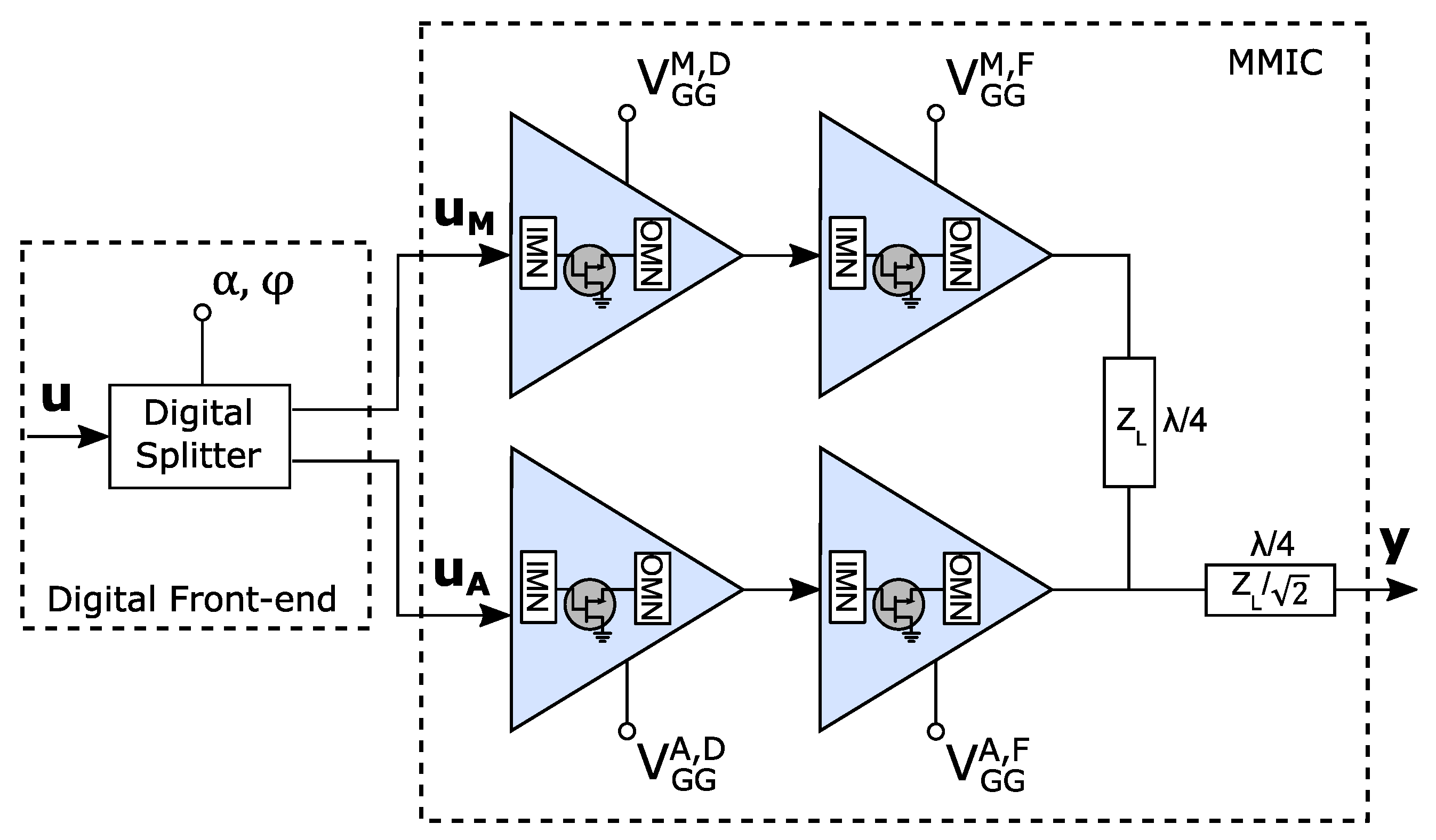
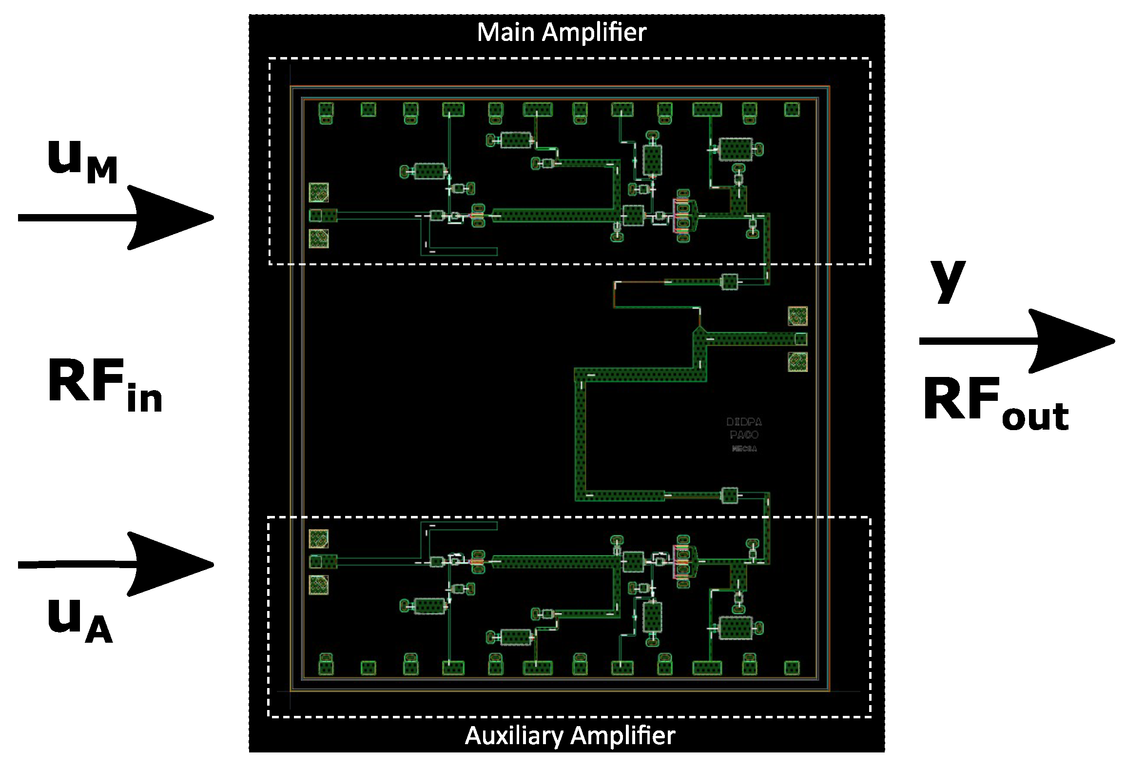
2.1. DIDPA Design
2.2. Definition of the Optimization Problem
2.3. Surrogate Modeling and Considerations for Linearity with Modulated Signals
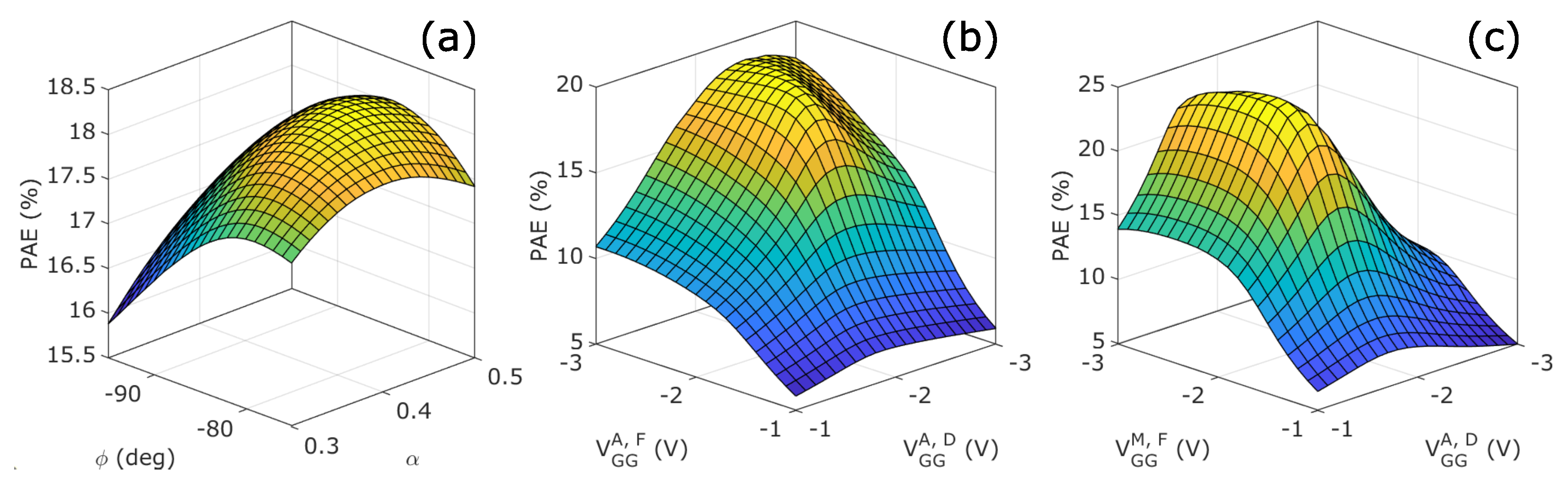
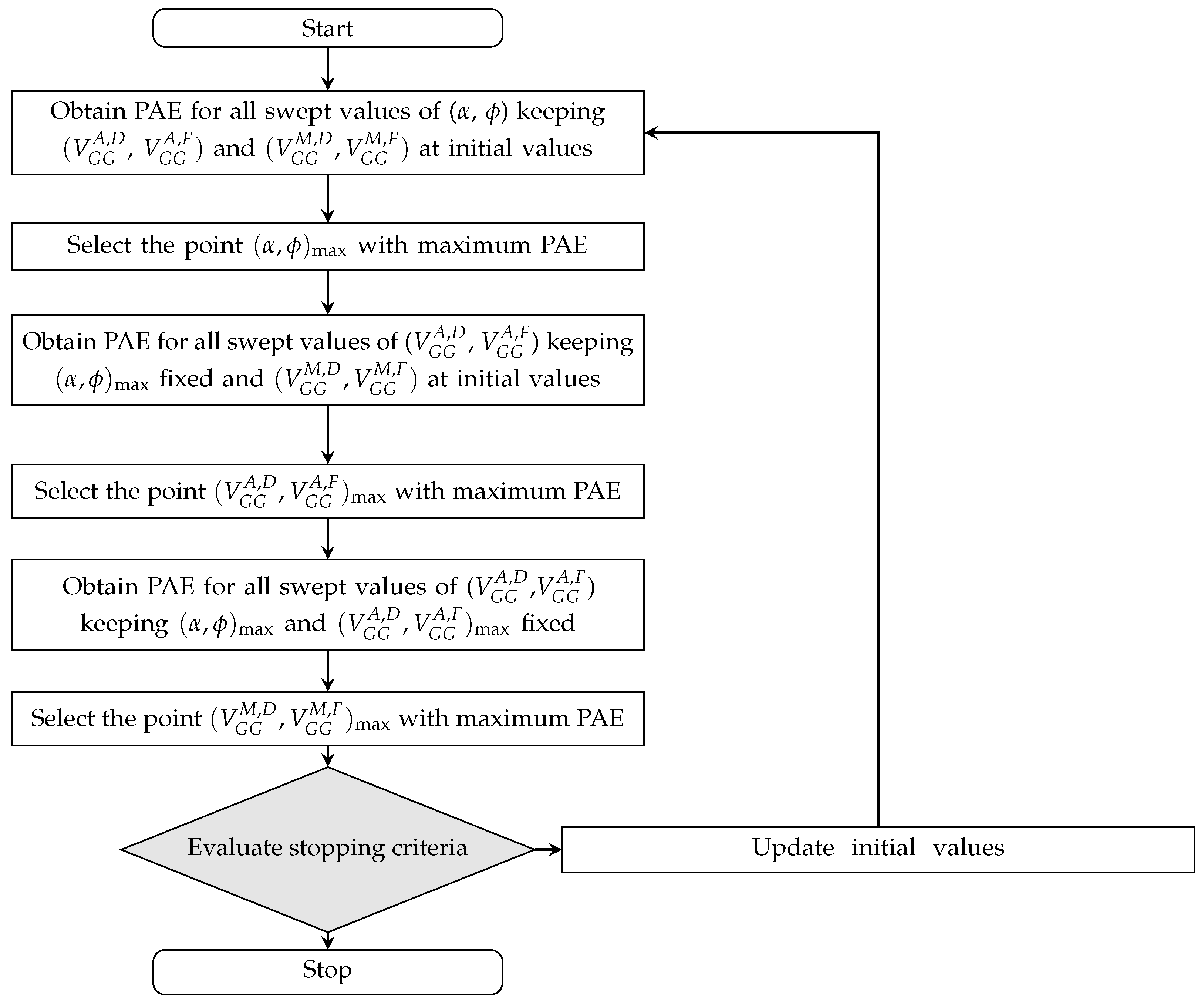
3. Coordinate Descent Optimization
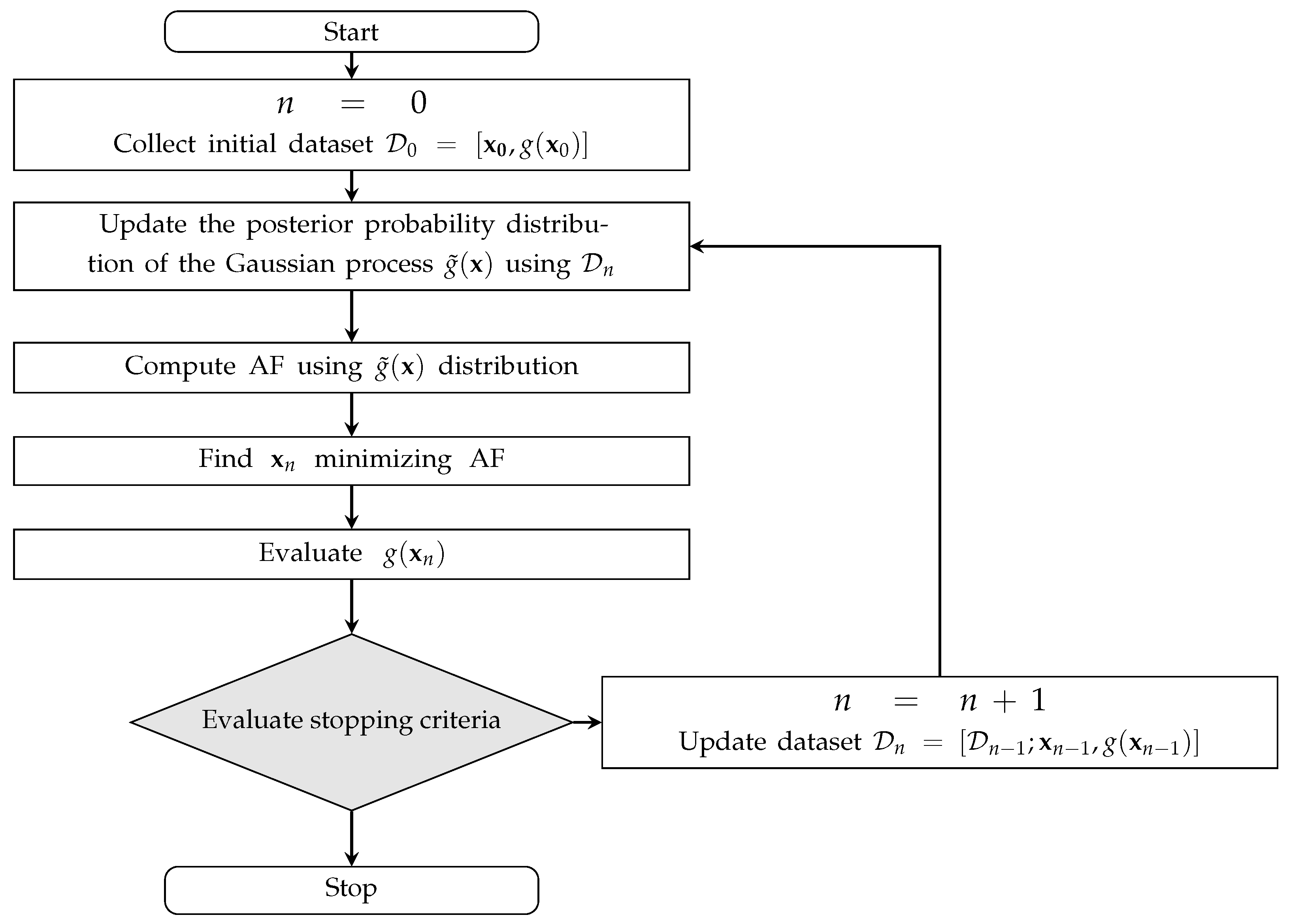
4. Bayesian Optimization
- A parametric model for the Gaussian process covariance function. The parameters of this model represent the hyperparameters of the SUMO, which are updated at every iteration using the samples of . The basis functions that are typically used in these applications are the radial basis functions or squared exponential functions. In this work, the covariance model is based on the Matern functions (the Matern functions are the default basis functions adopted by the MATLAB bayesopt routine used in this work) [28].
- The acquisition function (AF) is used to estimate the location of the minimum/maximum of interest. Since the RGM does not provide a deterministic value for the SUMO estimation, it is necessary to choose a function that selects the predicted value among all possible ones. Therefore, the AF takes the stochastic process as the input, and it provides a deterministic function, whose minimum/maximum is the point that will be evaluated by the objective function. One possible strategy is to choose the AF that calculates the expected improvement or the probability of improvement in the evaluated point [29]. The AF used in this work is called lower confidence bound:where and are, respectively, the mean and the variance of the Gaussian process in the evaluated point , while w is a scalar parameter used to select the tradeoff between exploring unknown points or searching new optima close to the previously expected ones.
5. Multi-Objective Bayesian Optimization
6. DIDPA Performance under Wideband Modulation
Author Contributions
Funding
Institutional Review Board Statement
Informed Consent Statement
Data Availability Statement
Acknowledgments
Conflicts of Interest
References
- Lavrador, P.M.; Cunha, T.R.; Cabral, P.M.; Pedro, J. The linearity-efficiency compromise. IEEE Microw. Mag. 2010, 11, 44–58. [Google Scholar] [CrossRef]
- Chen, W.; Lv, G.; Liu, X.; Wang, D.; Ghannouchi, F.M. Doherty PAs for 5G massive MIMO: Energy-efficient integrated DPA MMICs for sub-6-GHz and mm-wave 5G massive MIMO systems. IEEE Microw. Mag. 2020, 21, 78–93. [Google Scholar] [CrossRef]
- Piacibello, A.; Giofrè, R.; Quaglia, R.; Figueiredo, R.; Carvalho, N.; Colantonio, P.; Valenta, V.; Camarchia, V. A 5-W GaN Doherty Amplifier for Ka-Band Satellite Downlink With 4-GHz Bandwidth and 17-dB NPR. IEEE Microw. Wirel. Components Lett. 2022. [Google Scholar] [CrossRef]
- Marchetti, M.; Pelk, M.J.; Buisman, K.; Neo, W.E.; Spirito, M.; de Vreede, L.C. Active harmonic load–pull with realistic wideband communications signals. IEEE Trans. Microw. Theory Tech. 2008, 56, 2979–2988. [Google Scholar] [CrossRef]
- Hallberg, W.; Nopchinda, D.; Fager, C.; Buisman, K. Emulation of Doherty amplifiers using single-amplifier load–pull measurements. IEEE Microw. Wirel. Components Lett. 2019, 30, 47–49. [Google Scholar] [CrossRef]
- Angelotti, A.M.; Gibiino, G.P.; Nielsen, T.S.; Schreurs, D.; Santarelli, A. Wideband active load–pull by device output match compensation using a vector network analyzer. IEEE Trans. Microw. Theory Tech. 2020, 69, 874–886. [Google Scholar] [CrossRef]
- Darraji, R.; Ghannouchi, F.M.; Hammi, O. A dual-input digitally driven Doherty amplifier architecture for performance enhancement of Doherty transmitters. IEEE Trans. Microw. Theory Tech. 2011, 59, 1284–1293. [Google Scholar] [CrossRef]
- Barton, T. Not just a phase: Outphasing power amplifiers. IEEE Microw. Mag. 2016, 17, 18–31. [Google Scholar] [CrossRef]
- Freiberger, K.; Wolkerstorfer, M.; Enzinger, H.; Vogel, C. Digital predistorter identification based on constrained multi-objective optimization of WLAN standard performance metrics. In Proceedings of the 2015 IEEE International Symposium on Circuits and Systems (ISCAS), Lisbon, Portugal, 24–27 May 2015; pp. 862–865. [Google Scholar]
- Li, L.; Ghazi, A.; Boutellier, J.; Anttila, L.; Valkama, M.; Bhattacharyya, S.S. Evolutionary multiobjective optimization for digital predistortion architectures. In Proceedings of the International Conference on Cognitive Radio Oriented Wireless Networks, Rome, Italy, 25–26 November 2016; pp. 498–510. [Google Scholar]
- Mengozzi, M.; Gibiino, G.P.; Angelotti, A.M.; Florian, C.; Santarelli, A. Supply-modulated PA performance enhancement by joint optimization of RF input and supply control. In Proceedings of the IEEE Asia-Pacific Microwave Conference, Hong Kong, China, 8–11 December 2020; pp. 585–587. [Google Scholar]
- Mengozzi, M.; Gibiino, G.P.; Angelotti, A.M.; Florian, C.; Santarelli, A. GaN power amplifier digital predistortion by multi-objective optimization for maximum RF output power. Electronics 2021, 10, 244. [Google Scholar] [CrossRef]
- Mengozzi, M.; Angelotti, A.M.; Gibiino, G.P.; Florian, C.; Santarelli, A. Joint Dual-Input Digital Predistortion of Supply-Modulated RF PA by Surrogate-Based Multi-Objective Optimization. IEEE Trans. Microw. Theory Tech. 2021, 70, 35–49. [Google Scholar] [CrossRef]
- Kantana, C.; Ma, R.; Benosman, M.; Komatsuzaki, Y. A Hybrid Heuristic Search Control Assisted Optimization of Dual-Input Doherty Power Amplifier. In Proceedings of the European Microwave Conference 2021, London, UK, 27–29 September 2022; pp. 126–129. [Google Scholar]
- Wang, T.; Li, W.; Quaglia, R.; Gilabert, P.L. Machine-Learning Assisted Optimisation of Free-Parameters of a Dual-Input Power Amplifier for Wideband Applications. Sensors 2021, 21, 2831. [Google Scholar] [CrossRef] [PubMed]
- Campbell, C.F.; Tran, K.; Kao, M.Y.; Nayak, S. A K-band 5W Doherty amplifier MMIC utilizing 0.15 μm GaN on SiC HEMT technology. In Proceedings of the 2012 IEEE Compound Semiconductor Integrated Circuit Symposium (CSICS), La Jolla, CA, USA, 14–17 October 2012; pp. 1–4. [Google Scholar]
- Valenta, V.; Davies, I.; Ayllon, N.; Seyfarth, S.; Angeletti, P. High-gain GaN Doherty power amplifier for Ka-band satellite communications. In Proceedings of the 2018 IEEE Topical Conference on RF/Microwave Power Amplifiers for Radio and Wireless Applications (PAWR), Anaheim, CA, USA, 14–17 January 2018; pp. 29–31. [Google Scholar]
- Nakatani, K.; Yamaguchi, Y.; Komatsuzaki, Y.; Sakata, S.; Shinjo, S.; Yamanaka, K. A Ka-band high efficiency Doherty power amplifier MMIC using GaN-HEMT for 5G application. In Proceedings of the 2018 IEEE MTT-S International Microwave Workshop Series on 5G Hardware and System Technologies (IMWS-5G), Dublin, Ireland, 30–31 August 2018; pp. 1–3. [Google Scholar]
- Shepphard, D.J.; Powell, J.; Cripps, S.C. An efficient broadband reconfigurable power amplifier using active load modulation. IEEE Microw. Wirel. Components Lett. 2016, 26, 443–445. [Google Scholar] [CrossRef]
- Barmuta, P.; Gibiino, G.P.; Ferranti, F.; Lewandowski, A.; Schreurs, D.M.P. Design of experiments using centroidal Voronoi tessellation. IEEE Trans. Microw. Theory Tech. 2016, 64, 3965–3973. [Google Scholar] [CrossRef]
- Miettinen, K. Nonlinear Multiobjective Optimization; Springer Science & Business Media: Berlin/Heidelberg, Germany, 2012; Volume 12. [Google Scholar]
- Cidronali, A.; Giovannelli, N.; Vlasits, T.; Hernaman, R.; Manes, G. A 240W dual-band 870 and 2140 MHz envelope tracking GaN PA designed by a probability distribution conscious approach. In Proceedings of the IEEE MTT-S International Microwave Symposium Digest, Natal, Brazil, 5–10 June 2011; pp. 1–4. [Google Scholar]
- Angelotti, A.M.; Gibiino, G.P.; Nielsen, T.S.; Santarelli, A.; Verspecht, J. It refers to a wrong edition of the conference. In Proceedings of the ARFTG Microwave Measurement Conference, Denver, CO, USA, 24 June 2022; pp. 1–4. [Google Scholar]
- Rolain, Y.; Zyari, M.; van Nechel, E.; Vandersteen, G. A measurement-based error-vector-magnitude model to assess non linearity at the system level. In Proceedings of the 2017 IEEE MTT-S International Microwave Symposium (IMS), Honolulu, HI, USA, 4–9 June 2017; pp. 1429–1432. [Google Scholar]
- Gibiino, G.P.; Santarelli, A.; Schreurs, D.; Filicori, F. Two-input nonlinear dynamic model inversion for the linearization of envelope-tracking RF PAs. IEEE Microw. Wirel. Components Lett. 2016, 27, 79–81. [Google Scholar] [CrossRef]
- Chani-Cahuana, J.; Landin, P.N.; Fager, C.; Eriksson, T. Iterative Learning Control for RF power amplifier linearization. IEEE Trans. Microw. Theory Tech. 2016, 64, 2778–2789. [Google Scholar] [CrossRef]
- Frazier, P.I. A Tutorial on Bayesian Optimization. arXiv 2018, arXiv:1807.02811. [Google Scholar]
- Rasmussen, C.E.; Williams, C.K.I. Gaussian Processes for Machine Learning; Adaptive Computation and Machine Learning; MIT Press: Cambridge, MA, USA, 2006; pp. 1–248. [Google Scholar]
- Snoek, J.; Larochelle, H.; Adams, R.P. Practical Bayesian Optimization of Machine Learning Algorithms. arXiv 2012, arXiv:1206.2944v2. [Google Scholar]
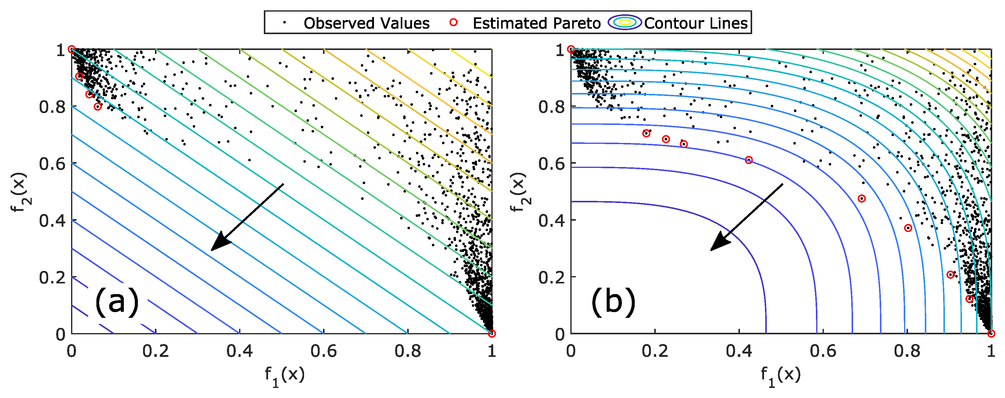
- Lafleur, J.M. Heuristic Method for Identifying Concave Pareto Frontiers in Multi-Objective Dynamic Programming Problems. AIAA J. 2014, 52, 496–503. [Google Scholar] [CrossRef]
- Angelotti, A.M.; Gibiino, G.P.; Florian, C.; Santarelli, A. Broadband error vector magnitude characterization of a GaN power amplifier using a vector network analyzer. In Proceedings of the IEEE/MTT-S International Microwave Symposium Digest, Los Angeles, CA, USA, 4–6 June 2020; pp. 747–750. [Google Scholar]


| (deg) | (V) | (V) | (V) | (V) | |
|---|---|---|---|---|---|
| 0.5 | −90 | −1.7 | −1.7 | −2.3 | −2.1 |
| (deg) | (V) | (V) | (V) | (V) | |
|---|---|---|---|---|---|
| 0.01 | 1 | 0.1 | 0.1 | 0.1 | 0.1 |
| Coordinate Descent Order | (dBm) | (%) |
|---|---|---|
| (,) → (,) → (,) | 24.0 | 24.5 |
| (,) → (,) → (,) | 23.9 | 24.1 |
| (,) → (,) → (,) | 24.2 | 24.3 |
| (,) → (,) → (,) | 24.0 | 25.2 |
| (,) → (,) → (,) | 23.8 | 25.0 |
| (,) → (,) → (,) | 23.9 | 25.3 |
| Algorithm | (dBm) | (%) | Nr of PAE Evaluations |
|---|---|---|---|
| Nominal (no optim) | 24.2 | 18.2 | – |
| Coordinate descent (,) → (,) → (,) | 23.9 | 25.3 | 1730 |
| Coordinate descent (iterated) (,) → (,) → (,) | 23.4 | 26.2 | 10,380 |
| Bayesian | 23.6 | 26.1 | 100 |
| Algorithm | (dBm) | (%) | Nr of Function Evaluations | |
|---|---|---|---|---|
| Nominal | ||||
| (no optim) | – | 24.2 | 18.2 | – |
| Coordinate descent (iterated) | – | 23.4 | 26.2 | 10,380 |
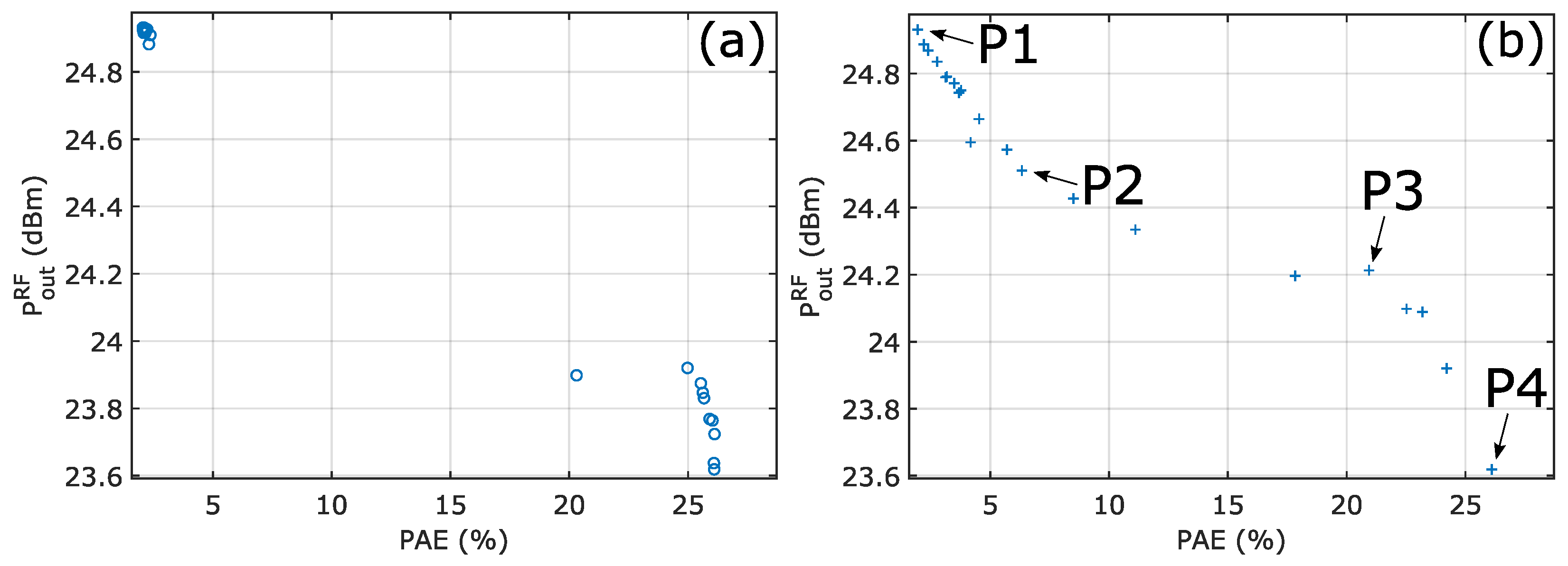
| Bayesian P1 | 0 | 24.9 | 2.0 | 100 |
| Bayesian P2 | 0.16 | 24.5 | 6.3 | 100 |
| Bayesian P3 | 0.84 | 24.2 | 20.0 | 100 |
| Bayesian P4 | 1 | 23.6 | 26.1 | 100 |
| Algorithm | (dBm) | (%) | (dB) | (dB) | |
|---|---|---|---|---|---|
| Nominal | – | 23.8 | 16.7 | ||
| Coordinate descent (best permutation) | – | 23.5 | 24.0 | ||
| Coordinate descent (iterated) | – | 23.4 | 24.6 | ||
| Bayesian P1 | 0 | 25.0 | 2.0 | ||
| Bayesian P2 | 0.16 | 24.1 | 6.0 | ||
| Bayesian P3 | 0.84 | 23.7 | 20.0 | ||
| Bayesian P4 | 1 | 23.4 | 24.6 |
| Algorithm | (deg) | (V) | (V) | (V) | (V) | |
|---|---|---|---|---|---|---|
| Nominal | 0.5 | |||||
| Coordinate descent (best permutation) | 0.5 | |||||
| Coordinate descent (iterated) | 0.6 | |||||
| Bayesian P1 | 0.49 | |||||
| Bayesian P2 | 0.21 | |||||
| Bayesian P3 | 0.43 | |||||
| Bayesian P4 | 0.61 |
Publisher’s Note: MDPI stays neutral with regard to jurisdictional claims in published maps and institutional affiliations. |
© 2022 by the authors. Licensee MDPI, Basel, Switzerland. This article is an open access article distributed under the terms and conditions of the Creative Commons Attribution (CC BY) license (https://creativecommons.org/licenses/by/4.0/).
Share and Cite
Mengozzi, M.; Gibiino, G.P.; Angelotti, A.M.; Santarelli, A.; Florian, C.; Colantonio, P. Automatic Optimization of Input Split and Bias Voltage in Digitally Controlled Dual-Input Doherty RF PAs. Energies 2022, 15, 4892. https://doi.org/10.3390/en15134892
Mengozzi M, Gibiino GP, Angelotti AM, Santarelli A, Florian C, Colantonio P. Automatic Optimization of Input Split and Bias Voltage in Digitally Controlled Dual-Input Doherty RF PAs. Energies. 2022; 15(13):4892. https://doi.org/10.3390/en15134892
Chicago/Turabian StyleMengozzi, Mattia, Gian Piero Gibiino, Alberto Maria Angelotti, Alberto Santarelli, Corrado Florian, and Paolo Colantonio. 2022. "Automatic Optimization of Input Split and Bias Voltage in Digitally Controlled Dual-Input Doherty RF PAs" Energies 15, no. 13: 4892. https://doi.org/10.3390/en15134892