
Evaluation Method of Naturalistic Driving Behaviour for Shared-Electrical Car

1
College of Energy and Power Engineering, Shandong University, Jinan 250061, China
2
Department of Mechanical Engineering Sciences, University of Surrey, Guildford GU2 7XH, UK
3
Research Management Department, Hisense TransTech Co., Ltd., Qingdao 266071, China
*
Author to whom correspondence should be addressed.
Energies 2022, 15(13), 4625; https://doi.org/10.3390/en15134625
Submission received: 10 May 2022
/
Revised: 18 June 2022
/
Accepted: 22 June 2022
/
Published: 24 June 2022
(This article belongs to the Topic Zero Carbon Vehicles and Power Generation)
Abstract
:Evaluation of driving behaviour is helpful for policy development, and for designing infrastructure and an intelligent safety system for a car. This study focused on a quantitative evaluation method of driving behaviour based on the shared-electrical car. The data were obtained from the OBD interface via CAN bus and transferred to a server by 4G network. Eleven types of NDS data were selected as the indexes for driving behaviour evaluation. Kullback–Leibler divergence was calculated to confirm the minimum data quantity and ensure the effectiveness of the analysis. The distribution of the main driving behaviour parameters was compared and the change trend of the parameters was analysed in conjunction with car speed to identify the threshold for recognition of aberrant driving behaviour. The weights of indexes were confirmed by combining the analytic hierarchy process and entropy weight method. The scoring rule was confirmed according to the distribution of the indexes. A score-based evaluation method was proposed and verified by the driving behaviour data collected from randomly chosen drivers.
1. Introduction
Road accidents kill approximately 1.24 million people every year and they are the eighth leading cause of death globally [1]. Aberrant driving and violation of traffic rules cause 74% of traffic accidents [2]. In addition, these behaviours also lead to excessive fuel consumption and vehicle emissions [3]. Therefore, it is necessary to understand the influence of driving behaviour on road risks and vehicle performance. Additionally, quantitative methods of the aberrant driving behaviour should be proposed to improve the driving behaviour.
In former studies, driving behaviour data have been mainly obtained by the following methods: driver self-reported survey [4], driver behaviour questionnaires [5], driver simulators [6], field tests and Naturalistic Driving Studies (NDS) [7]. The first two methods are subjective evaluation methods. For the driver simulators and field tests, the driving behaviour may be different due to the pre-arranged test environment and procedure. Naturalistic driving data were obtained with an unobtrusive data acquisition system during everyday driving. NDS can observe the driving behaviour in a natural driving condition without experimental control. Therefore, the method can accurately reflect driving habits [8]. NDS can be categorized further into on-site study and individual driver study [9]. For the on-site study, naturalistic driving data can be collected with video cameras or microwave and other equipment at a particular site. The individual driver study can obtain various driving behaviour data, such as vehicle speed, acceleration, location and vehicle clearance and so on. For the individual driver study, abundant driving behaviour data can provide multi-dimensional analysis for driving behaviour.
NDS data from the study of individual drivers can be obtained by Global Position System (GPS), video cameras, independent sensors, mobile phones and On-Board Diagnostics (OBD). GPS can provide vehicle location directly and vehicle speed can be estimated based on the location. The acceleration and deceleration behaviour of drivers were studied using GPS in [10,11]. Video cameras were used to capture the drivers’ facial expressions and eye movements to analyse the driving behaviour [12]. Video cameras were also used to record drivers’ body movements, such as feet movements, to evaluate the reaction time of the drivers [13]. Independent sensors such as accelerometer [14], Radar sensor [15] and Inertial Measurement Unit (IMU) [16] were also used to obtain driving behaviour data. Nowadays, most mobile phones are equipped with GPS and an accelerometer. Driving behaviour such as acceleration, braking and speeding were studied using mobile phones in [17]. OBD II interface was mandatory for vehicles and the system can collect variable vehicle information from the Electronic Control Units (ECU) of the vehicles via the Controller Area Network (CAN) bus. OBD II interface can collect vehicle status and operation information, including vehicle speed, acceleration, position of accelerator/ brake pedal, angle of steering wheel and fuel consumption and so on [18]. Considering the abundant information and reliability of the OBD II, the data collected from OBD was used to analyse the driving behaviour [19].
Driving behaviour can be influenced by driver’s driving ability, driver characteristics, driving duration and driver’s distraction [20]. Driving ability was influenced by the driver’s experience, skill and knowledge. Compared with experienced drivers, young drivers had a higher rate of traffic accidents [21]. Driver characteristics include age, gender, and education level and etc. Drivers’ behaviour was influenced by the drivers’ age. Young drivers had a higher probability of accidents than middle-aged and older drivers due to their higher tendency of speeding [22]. Most studies showed that the drive behaviour of males was more aggressive that of than females and that males had higher risk of having an accident [23]. The behaviour of drivers with a high education level was more compliant, such as less lane-changing [24]. Driving duration had a significant influence on driving behaviour and there was more speeding for the drivers who had a longer driving distance [25]. A driver can be distracted by the driving environment, their mobile phone, their co-passenger and so on [26]. The distractions had adverse impacts on road safety, especially when the driver glanced away from the road.
Driving behaviour has a great influence on the road safety and vehicle performance. The evaluation of driving behaviour is helpful in providing positive feedback to drivers so they reduce the dangerous driving, thus avoiding traffic accidents and enhancing vehicle performance. According to the conclusion of the previous paragraph, driving behaviour is influenced by multiple factors. Considering the stochastic feature of the driving behaviour, it is better to extract the driving behaviour feature from a large sample, including the driver selection and driving route. Nowadays, shared-electrical cars are used in several cities in China, the driver and driving route are random for each trip, and the driving behaviour is purely naturalistic. The driving behaviour data contains drivers of different ages, genders and driving experiences. This makes it suitable for the evaluation of the driving behaviour. While there have been a few studies that have conducted an evaluation of the driving behaviour using data from shared-electrical cars, the statistical characteristics of NDS data with a large and stochastic sample is still unclear, and should be studied in more depth.
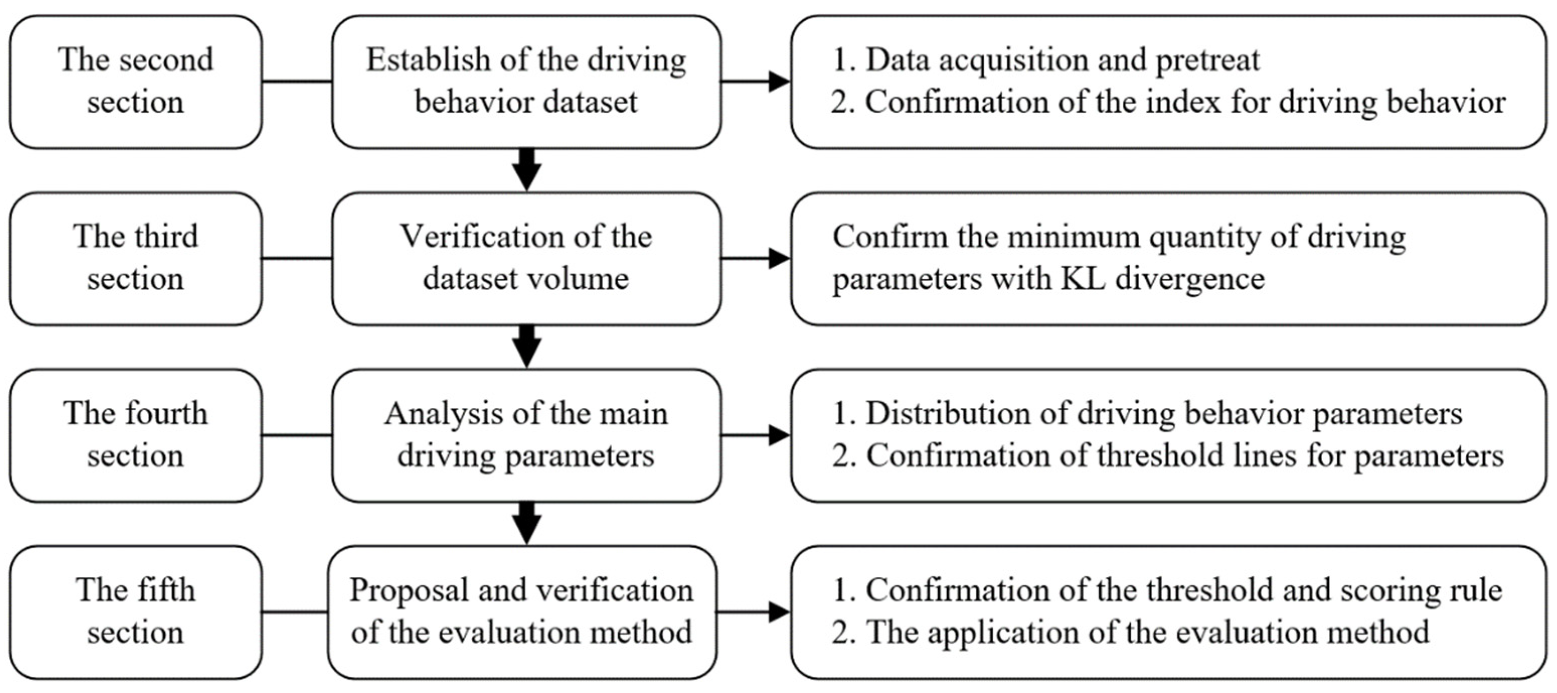
To bridge the knowledge gap, this paper was conducted using the data from shared-electrical cars used in Shanghai and Tianjin cities of China. On this basis, a quantitative evaluation method of driving behaviour was proposed and verified. This paper was organized as follows. Firstly, the NDS data obtained from the OBD-II interface of the shared-electrical car was pre-treated to improve the data quality. Secondly, an estimation method was employed to confirm the appropriate amount of NDS data. Thirdly, the relationship between different driving behaviour parameters was studied. Finally, an evaluation of driving behaviour was proposed and verified in practical application. The study flow chart is shown in Figure 1.
2. Data Acquisition and Treatment
2.1. Data Acquisition
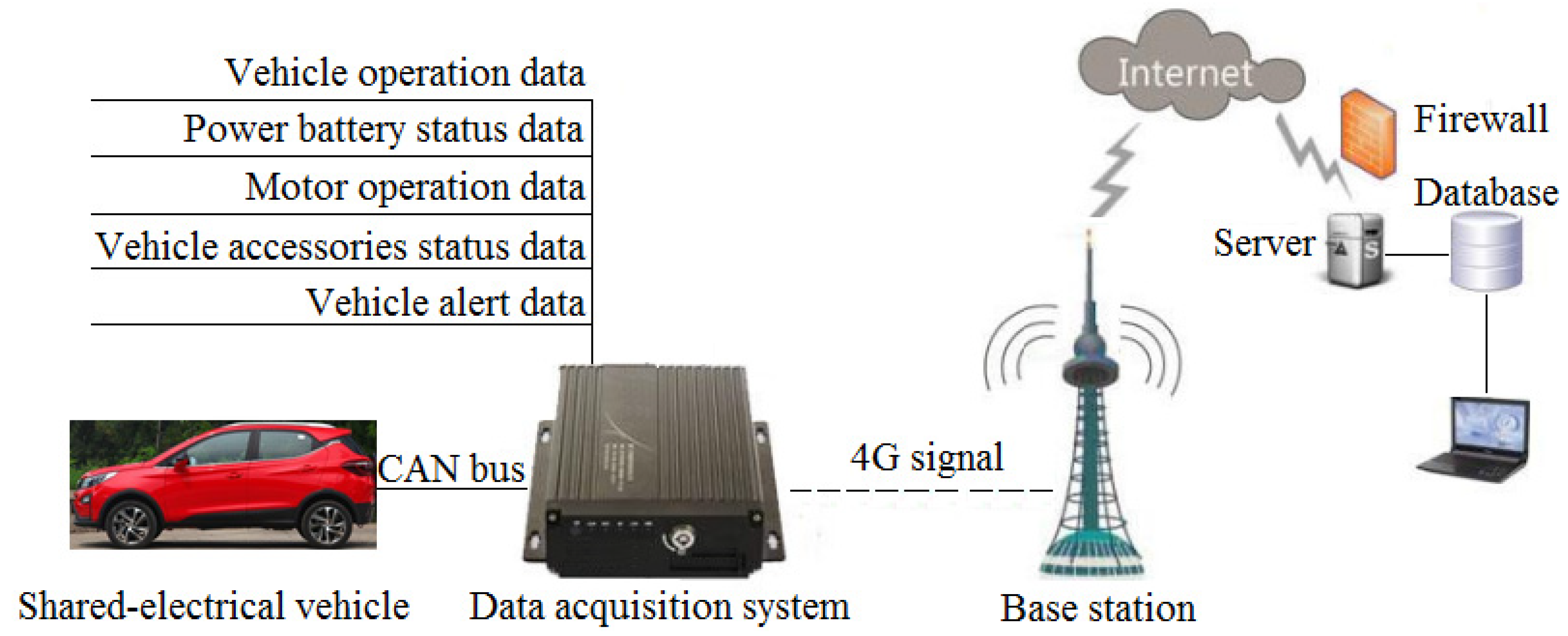
The NDS data were collected from 400 electrical cars, in which 305 cars were shared-electrical cars and others were online car-hiring cars. A data acquisition system was used to obtain the NDS data from the OBD-II interface via CAN bus. All the sampled data were sent to a server by a 4G network. The data were saved and treated thereafter for driving behaviour analysis. The data acquisition process is shown in Figure 2. The data were collected during a period of about four months. The total car mileage was about 1.2 million kilometres, with the total car travelling hours adding up to about 45,000, and the sample points totaling about .
The data acquisition system can obtain more than 50 driving behaviour parameters, including vehicle operation, power battery status, motor operation, vehicle accessories status and vehicle alert. The primary data were shown in Table 1. All the data were collected at a rate of 10 Hz, which was adequate for transient process analysis, such as acceleration or deceleration.
It should be noted that the collected data mentioned above were obtained from the OBD-II interface, and do not include any personal information, such as GPS data.
2.2. Data Treatment
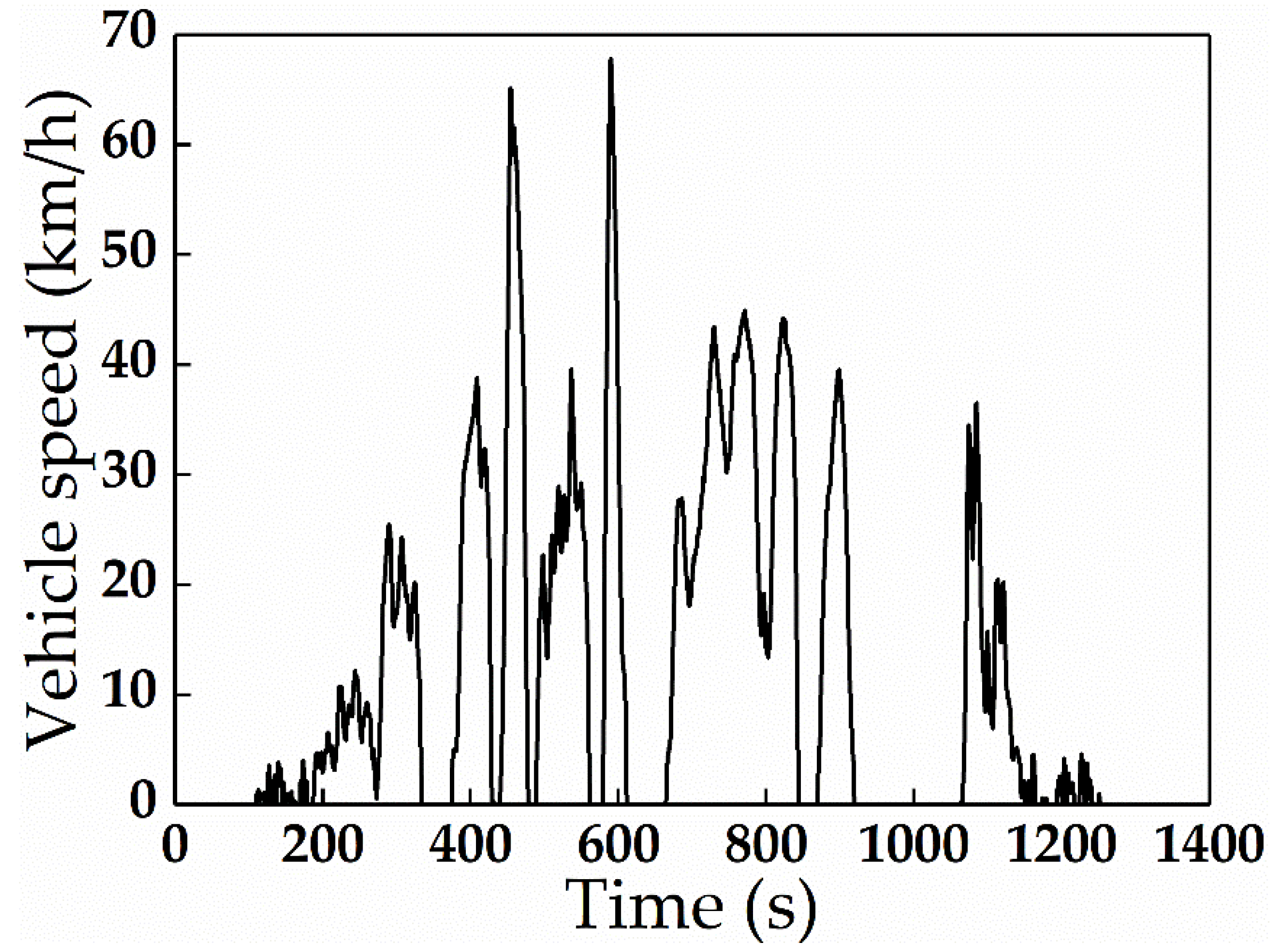
The vehicle data were collected in ‘Charge’, ‘Standby’ and ‘Operation’ phases. For the analysis of driving behaviour, the data collected in the ‘Charge’ and ‘Standby’ phases were neglected. A valid driving event was recognised by both the power-on status and the vehicle speed being greater than zero. When the vehicle speed was zero for less than 10 min with power-on status, it was considered in the same driving event. Figure 3 showed an example of the vehicle speed versus time in a complete driving event.
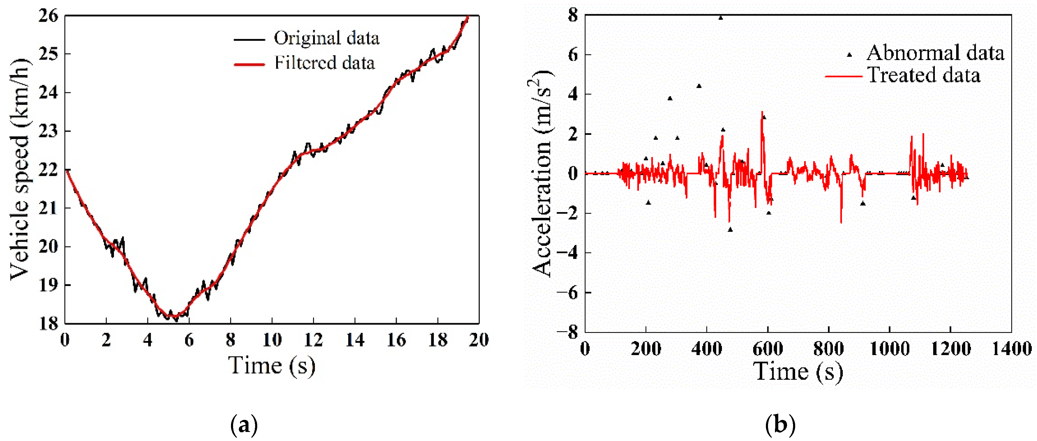
The data acquisition and transmission can be affected by occasional interferences, such as the voltage fluctuation in the vehicle start and stop phase, abnormal power failure of the data acquisition system, the interruption of the communication signal caused by tunnels or tall buildings and so on [27]. The data received by the server include occasional flaws; therefore, a data quality control method must be used before processing. The sliding-window averaging filter was implemented to reduce the random noise. The filter can be expressed as follows:
where is the number of the original data, is the original data, is the length of the sliding-window averaging filter, which is set to five, and is the treated data.
The vehicle data were obtained from the ECUs of the vehicles via CAN bus. Most of the data were deemed normal. To eliminate the occasional abnormal data, the box diagram method was used, which was introduced in the previous paper [28]. The sliding-window averaging filter and box diagram method were used to treat the original data. Figure 4a showed the treatment effect of the filter on vehicle velocity. It can be seen that the signal fluctuation was eliminated but the trend remained the same. Figure 4b showed the treatment effect of the box diagram method for the acceleration and the abnormal value can be eliminated effectively.
2.3. The Indexes for Driving Behaviour
There were multiple indexes to evaluate the driving behaviour. This study mainly focused on the indexes related to driving safety, including frequent adjustment of vehicle speed and steering wheel, rapid acceleration, sudden braking, rapid turning, fatigue driving and power consumption. The proposed evaluation method of driving behaviour was based on 11 indexes. The index, symbol, definition and unit are listed in Table 2. All values were calculated based on a complete driving event.
3. Quantity Estimation of Driving Behaviour Data
For an individual driver, the driving style is relatively stable after a certain period of driving experience and the statistical characteristics will be convergent [29]. The evaluation accuracy of driving behaviour depends on the volume of the NDS dataset, which should cover as many of the driving behaviour characteristics as possible. From the statistical perspective, if the NDS data are adequate, the distribution density of the data will remain the same with additional sample data. In this case, the amount of NDS data can be considered suitable for driving behaviour analysis. To ensure the appropriate quantity of dataset, the amount of NDS data was estimated by Kullback–Leibler (KL) divergence [30]. The quantity estimation of a given dataset included the following two steps.
Firstly, the distribution density () of the dataset was calculated with the kernel density method, which was a non-parametric method, and the equations are as follows.
where is the length of the dataset, is standard deviation of the dataset.
Secondly, the KL divergence was calculated to assess the difference in kernel density between the two datasets with the data length of n and respectively. Assuming the kernel densities of the two datasets are expressed as and , the KL divergence of the two datasets can be expressed as Equation (5). If KL remains as a small value with the increase in m, it indicates that the kernel density is almost unchanged with the adjustment of the dataset and the quantity of the dataset is adequate. The variation value of KL can affect the data quantity, which was set as KL in this study.
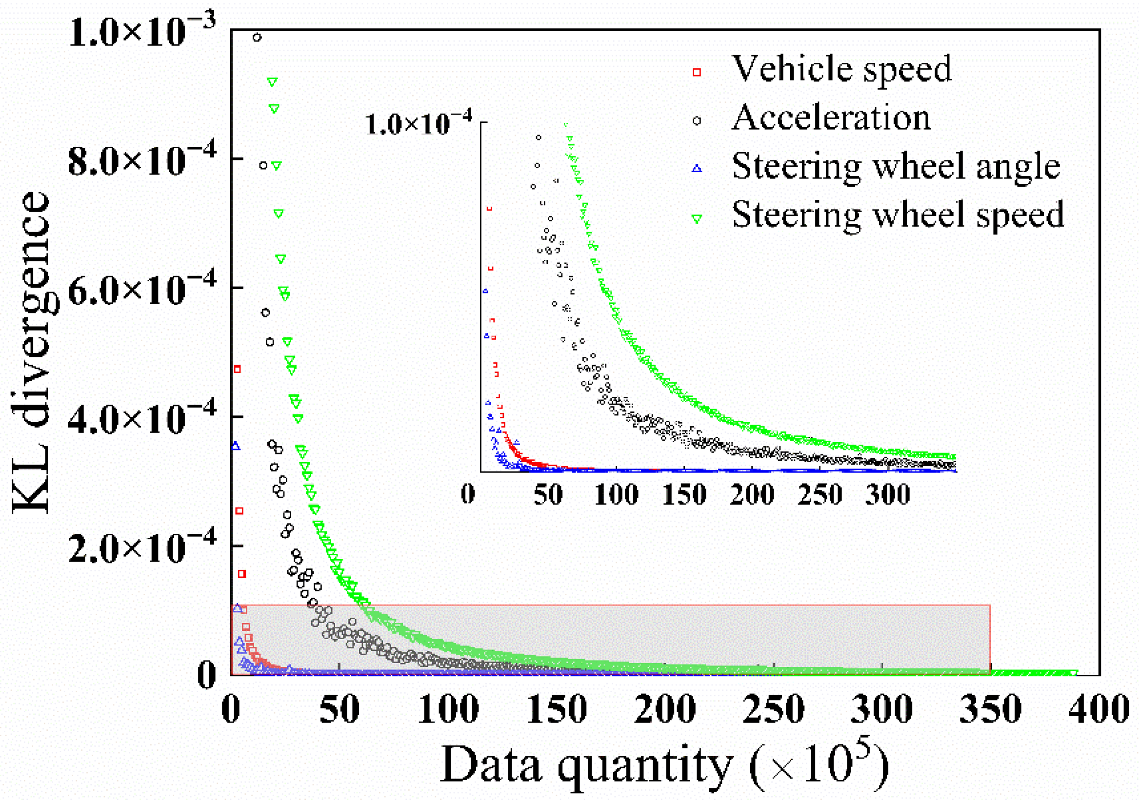
The KL divergence of different driving behaviour parameters was calculated and Figure 5 showed the changing trend of vehicle speed, acceleration, steering wheel angle and steering wheel speed. It can be seen that the KL of different parameters decreased with the increase in data quantity. Although the convergence rate of the parameters was different, the KL convergence of the four parameters all satisfied the requirement when the data quantity exceeded . The similar calculation of KL was applied to other driving behaviour parameters. Based on this analysis, the quantity of the sampled data in this study was considered adequate.
4. Study on the Relationship between Different Driving Behaviour Parameters
4.1. Statistical Characteristics of the Main Driving Behaviour Parameters
Vehicle speed, acceleration, deceleration, steering wheel angle and steering wheel speed contain abundant information reflecting driving behaviour. The statistics of these parameters were firstly calculated to understand the general characteristics of the driving behaviour.
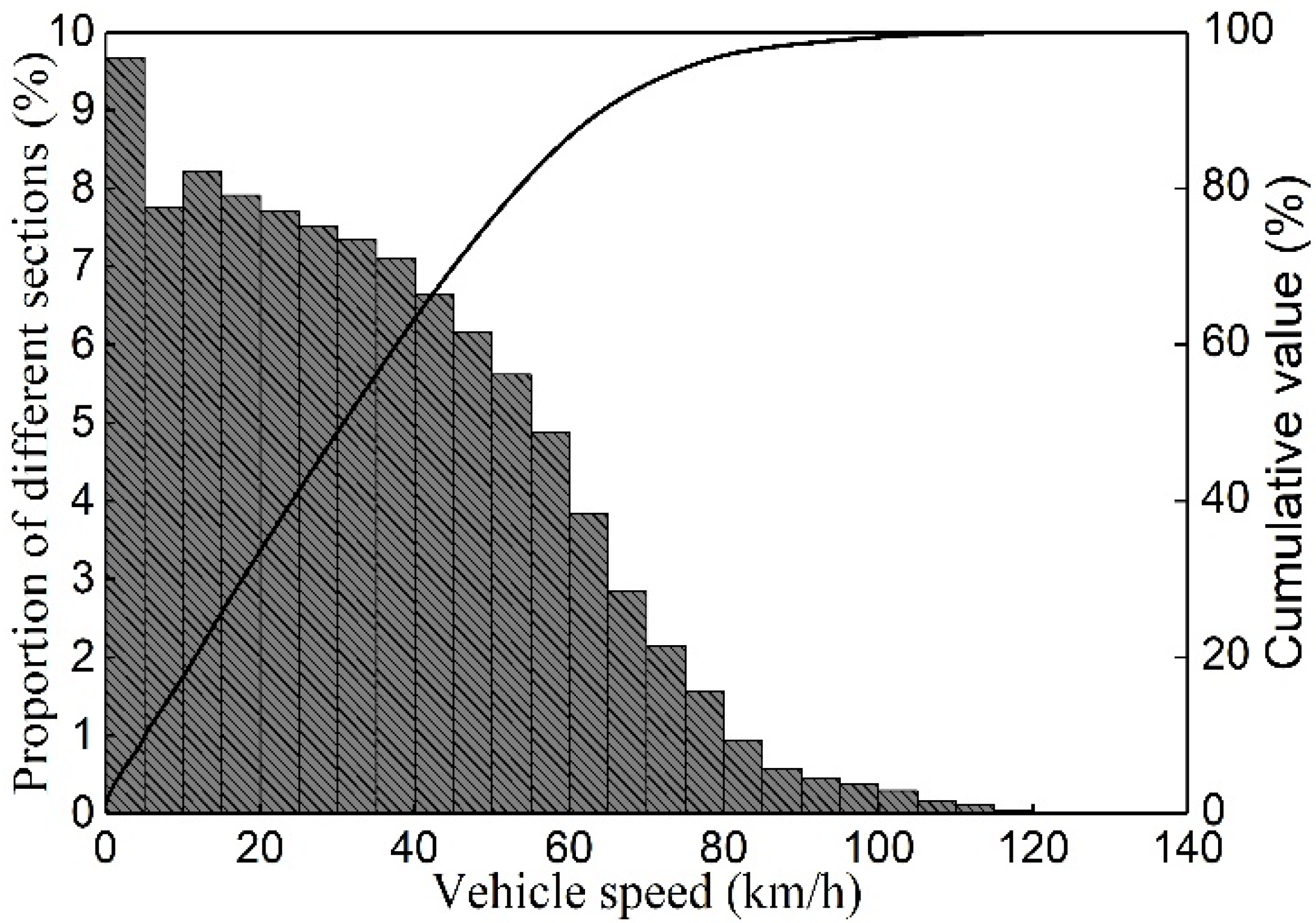
According to Figure 5, the KL of vehicle speed converged when the data quantity exceeded . The vehicle speed was selected randomly from the total dataset of shared-electrical vehicles to the quantity of . The distribution characteristic of the vehicle speed is shown in Figure 6. Most of the vehicles’ speeds were lower than 80 km/h and the average speed was 33.4 km/h. The relatively low speed was mainly attributed to the heavy urban traffic. The largest proportion of the speed was lower than 5 km/h, which reflected the frequent starting or parking mode due to red lights or traffic jams in urban traffic.
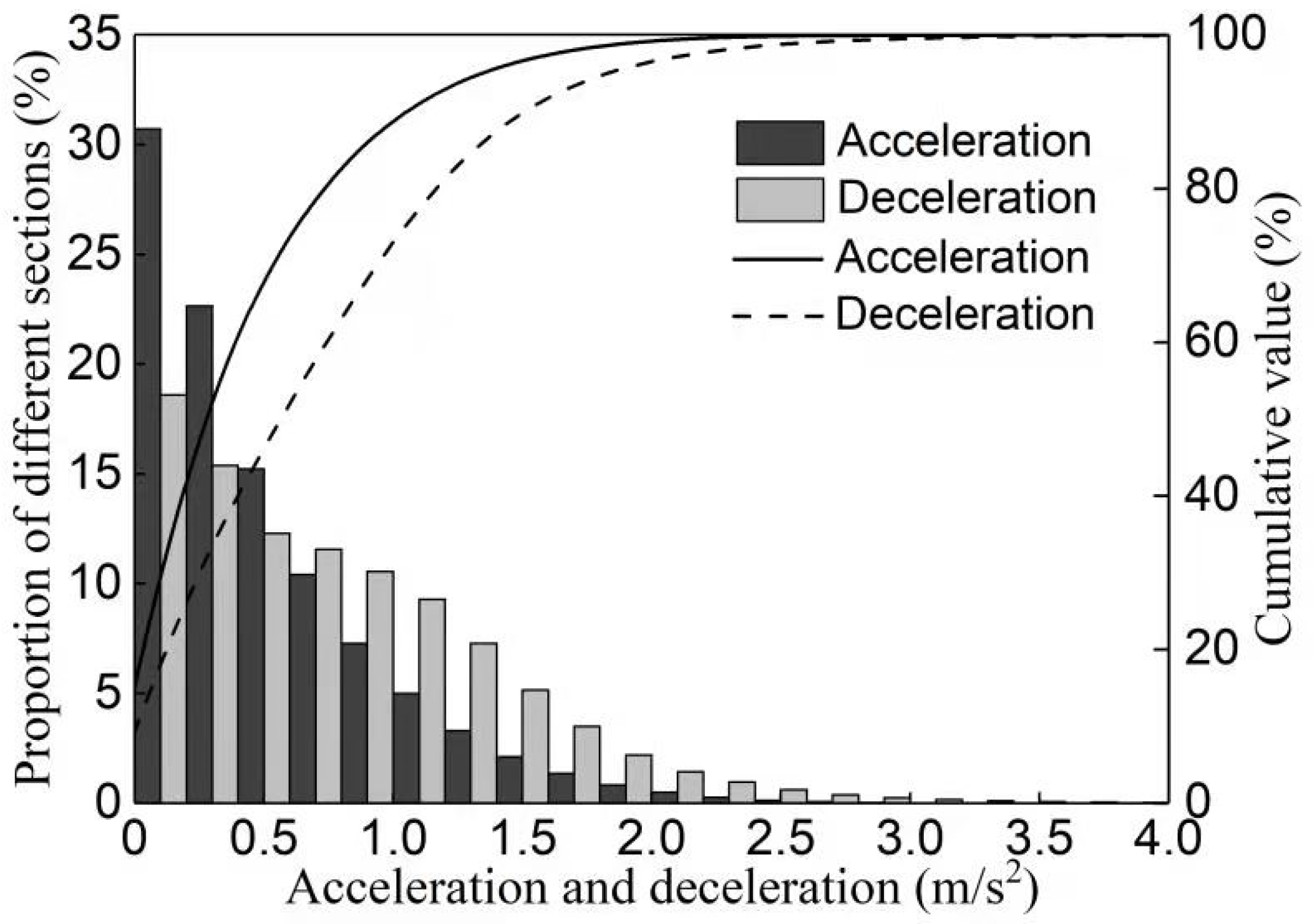
According to Figure 5, the KL of acceleration and deceleration converged when the data quantity exceeded . The corresponding data quantity of acceleration and deceleration were selected randomly from the total dataset of shared-electrical vehicle. The distribution characteristic was compared and shown in Figure 7. Over 90% of the acceleration and deceleration were lower than 1.5 m/s2. The average values of acceleration and deceleration were 2.05 and 2.72 m/s2, respectively. Compared to deceleration, acceleration was mainly located within the small value sections, which was mainly attributed to the heavy traffic.
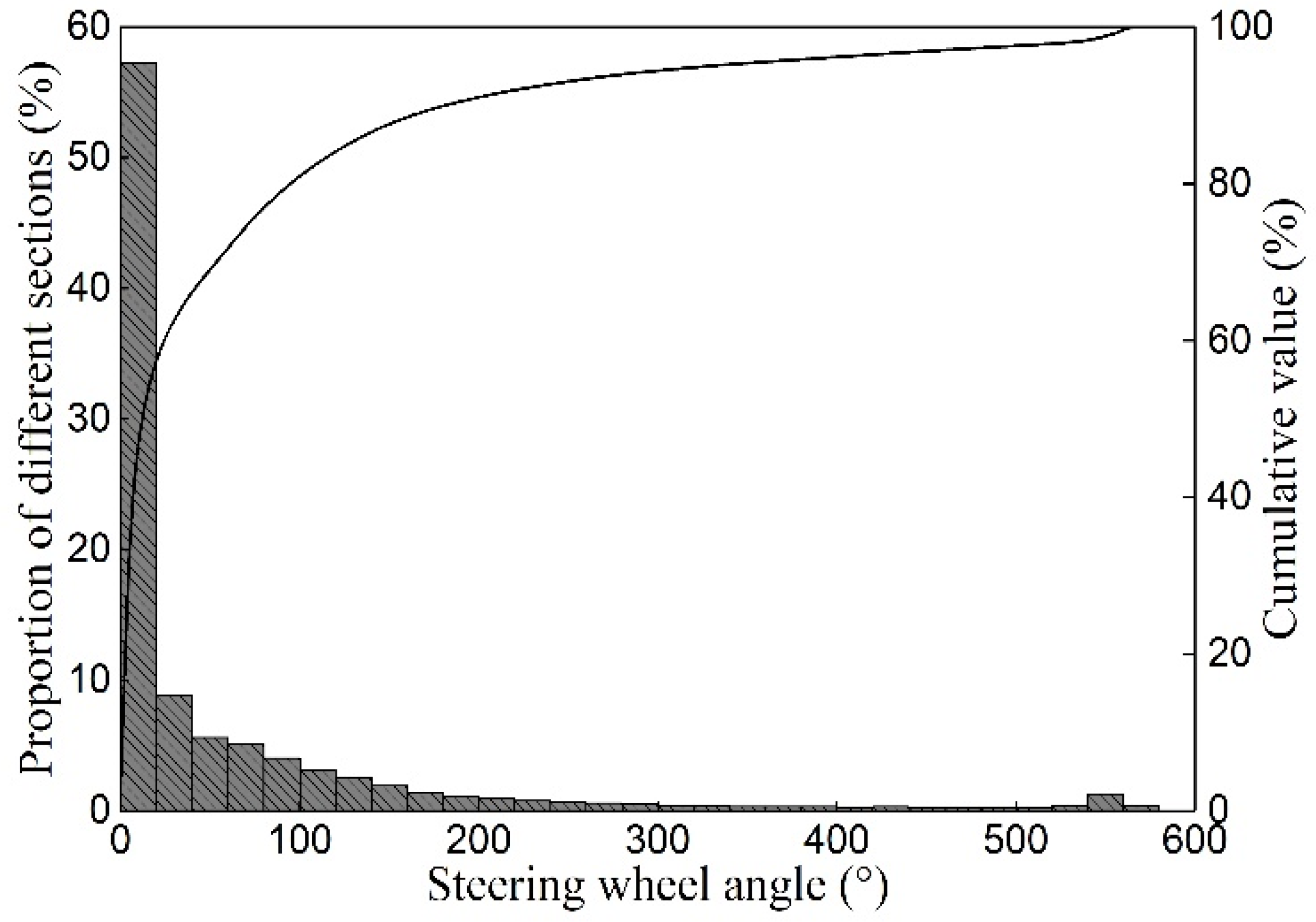
The KL of steering wheel angle converged when the data quantity was more than , and the corresponding quantity of steering wheel angle data was selected randomly. The distribution characteristic of steering wheel angle is shown in Figure 8. Over 60% of the steering wheel angle was lower than 25°, which meant that most of the angle change was attributed to the slight adjustment in driving direction. The percentage decreased with the increase in steering wheel angle until 300°, and these steering actions were mainly due to lane-changing or vehicle turning. There was also angle distribution around 550°, and this was mainly caused by vehicle U-turn or parking.
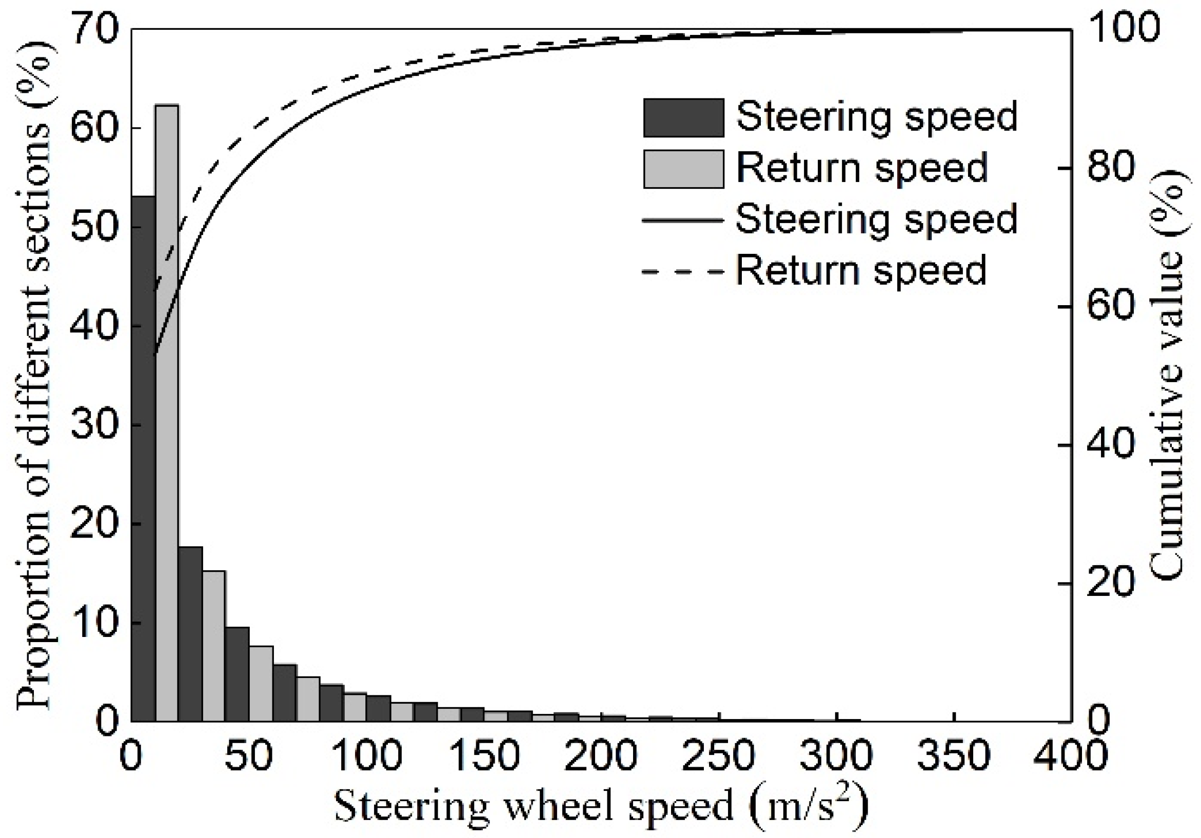
The KL of steering wheel speed converged when the data quantity was more than . The same amount of steering wheel speed data was selected randomly and compared in Figure 9. According to the steering characteristic, the steering wheel speed can be classified to steering speed (positive values) and return speed (negative values). Comparison showed that the two speeds had a similar changing pattern. Most of the steering speeds and return speeds were lower than 25°/s, which meant that the majority of the steering actions were careful. The averages of the steering speed and return speed were calculated, which were 38.11°/s and 30.35°/s, respectively. The steering speed was larger than the return speed, which corresponded to the normal driving habit.
4.2. Statistical Characteristics of Parameters at Different Vehicle Speed
The acceleration, deceleration, steering wheel angle and steering wheel speed are affected by vehicle speed. To reveal the influence of speed on different driving parameters, the statistical characteristics of the parameters at different vehicle speeds were analysed. The analysis can provide guidance for threshold settings of driving behaviour evaluation.
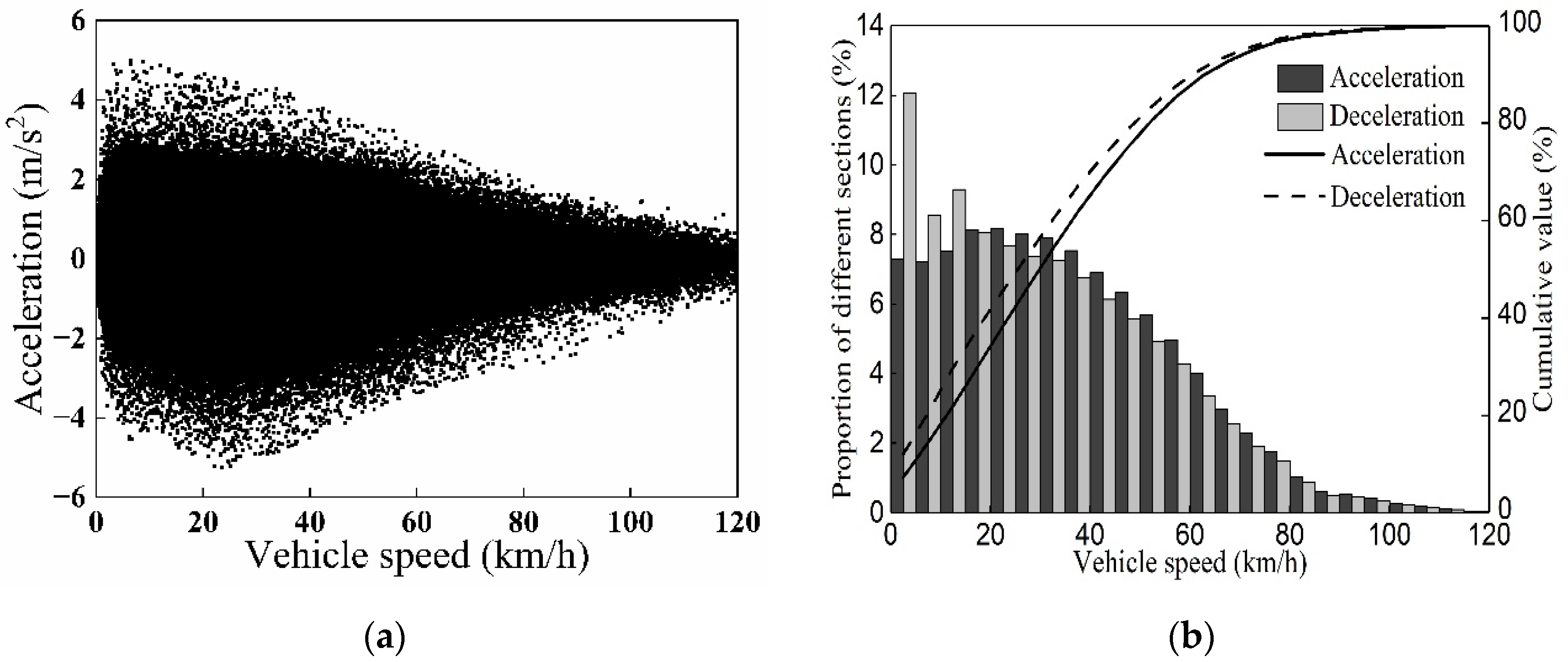
Figure 10a showed the distribution characteristic of acceleration and deceleration versus vehicle speed. The acceleration decreased, along with the increase in vehicle speed. The deceleration firstly increased and then decreased with the increase in vehicle speed, and the inflection point was approximately 25 km/h. An explanation of this scenario is introduced in the following section. The overall change trend suggested that the acceleration and deceleration approached zero with the increase in vehicle speed. This can be explained by the fact that the higher vehicle speeds normally appeared during smooth traffic and the vehicle speed change will reduce accordingly in this situation. Additionally, the drivers tended to keep the speed stable to ensure safety at high vehicle speeds. Figure 10b showed the distribution comparison of acceleration and deceleration at different vehicle speeds. The acceleration distribution was relatively stable in a wide range of vehicle speeds from 0 to 60 km/h and the largest proportion of acceleration appeared around the speed of 20 km/h, which was the vehicle starting condition. The deceleration was mainly distributed in the lower speed condition and the largest proportion of deceleration appeared at speeds ranging from 0 to 5 km/h.
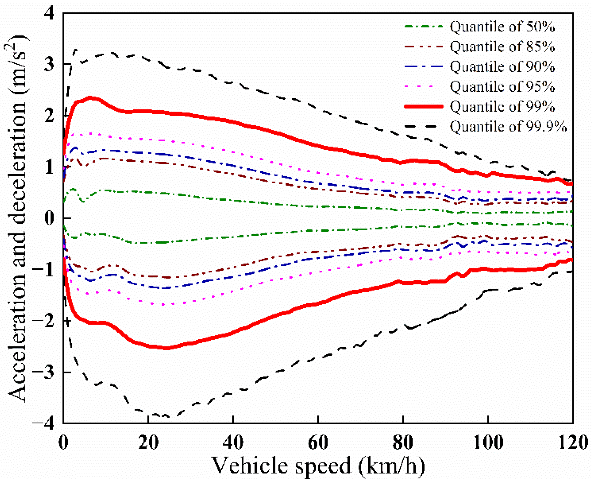
Figure 11 showed the different quantile values of acceleration and deceleration at different vehicle speeds. It can be seen that the acceleration increased significantly during the speed from 0 to 5 km/h, which was attributed to the electric motors’ high torque output at low speed. The quantile of the acceleration decreased with the increase in speed. This can be explained by the fact that the drivers tended to accelerate the vehicle more rapidly at lower speed conditions. The quantile of the deceleration firstly increased and then decreased. The reason for this is that the shared-electrical cars have braking energy recovery and the maximum braking torque appears at around 25 km/h, which led to this inflection point. The braking energy recovery in the deceleration phase was the main difference between the electrical vehicles and vehicles powered by Internal Combustion Engine (ICE).
To evaluate the abnormal acceleration or deceleration, some researchers employed the fixed threshold value. According to Figure 11, both the acceleration and deceleration tended to decrease with the increase in vehicle speed in general. Therefore, it was reasonable that the threshold of abnormal acceleration or deceleration changed with speed. To confirm the threshold, a linear fit was applied to the quantile of acceleration and deceleration during the speed range from 10 to 120 km/h. The linear fit of the acceleration is expressed as Equation (6).
where is vehicle speed and and are the coefficients of linear fit. The linear fit result is shown in Table 3, in which is the coefficient of determination.
Similarly, the quantile of deceleration also had a linear fitted. Considering the piece-wise characteristic of the deceleration, the piece-wise linear fit was employed, which is shown in Equation (7).
where is vehicle speed and , , and are the coefficients of linear fit. The linear fit result is shown in Table 4.
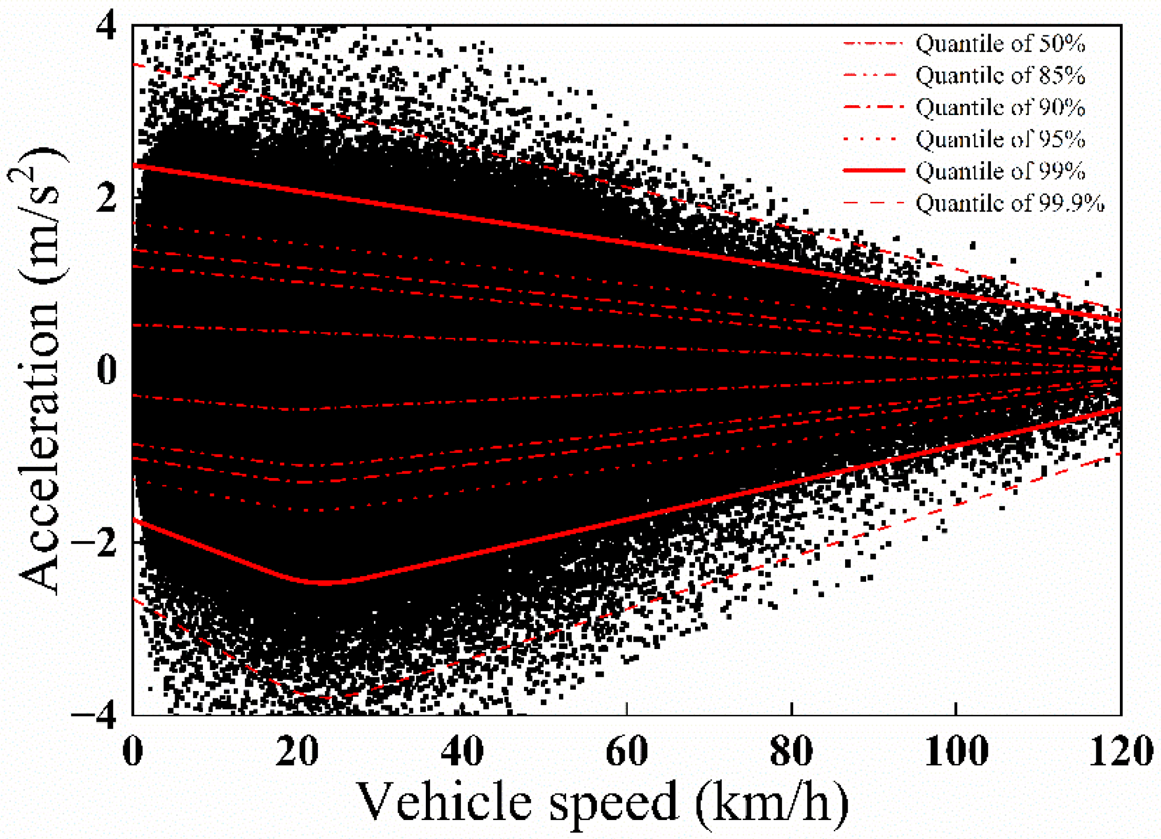
The linear fit result of the acceleration and deceleration were compared in Figure 12. Greater acceleration and deceleration can cause a feeling of discomfort and risk of traffic accidents. According to the quantile and distribution of acceleration and deceleration, the quantile value of 99% was arbitrarily employed to distinguish the abnormal acceleration and deceleration in the following evaluation of driving behaviour.
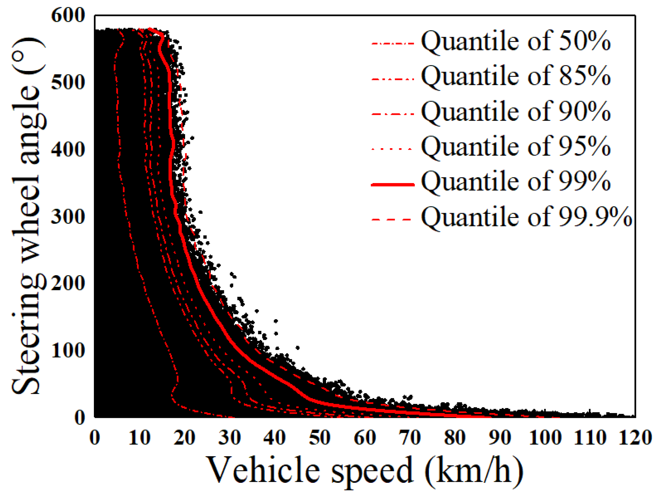
Vehicle speed has a great influence on driving safety and it is dangerous to steer heavily at high speeds. Figure 13 showed the comparison of distribution and quantile of steering wheel angle at different speeds. Most of the steering action occurred at the speed of 20 km/h, and the steering wheel angle decreased with the increase in speed. The trend corresponded to the driving habits that the steering demand was decreased with the increasing speed to ensure driving safety. The quantile value of the steering wheel angle was almost unchanged when the steering wheel angle was larger than 300°. This indicated that drivers tended to decrease vehicle speed at high steering angle conditions to avoid traffic accidents.
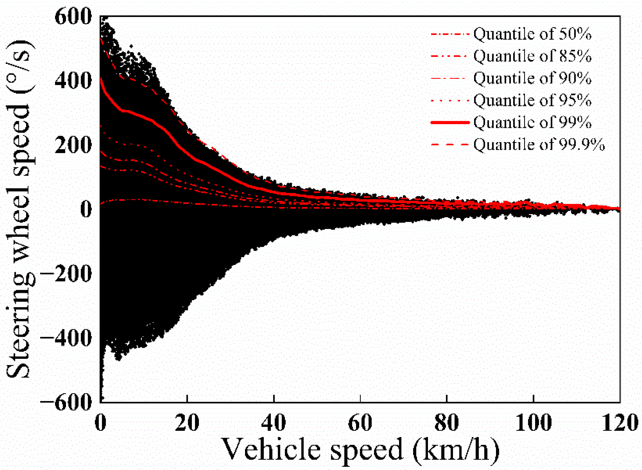
Rapid steering can reduce the lateral stability of vehicles. Steering wheel speed reflects the operation speed of the drivers on the steering wheels. A faster speed is usually associated with a higher risk of rollover and skid of the vehicle. Figure 14 showed the distribution of steering wheel speed versus vehicle speed. The maximum steering wheel speed can reach approximately 600°/s. The high steering wheel speeds mainly occurred at vehicle speeds lower than 30 km/h, which suggested that drivers tended to turn the steering wheel rapidly at safe speeds. The trends of steering speed and return speed were similar. They both decreased with the increase in vehicle speed. Considering the similar trend, the quantiles of the steering speed was obtained. The comparison of the quantile showed that the steering speed was almost unchanged when the vehicle speed was higher than 60 km/h, which meant that most of the steering actions were gentle at high vehicle speeds to ensure driving safety.
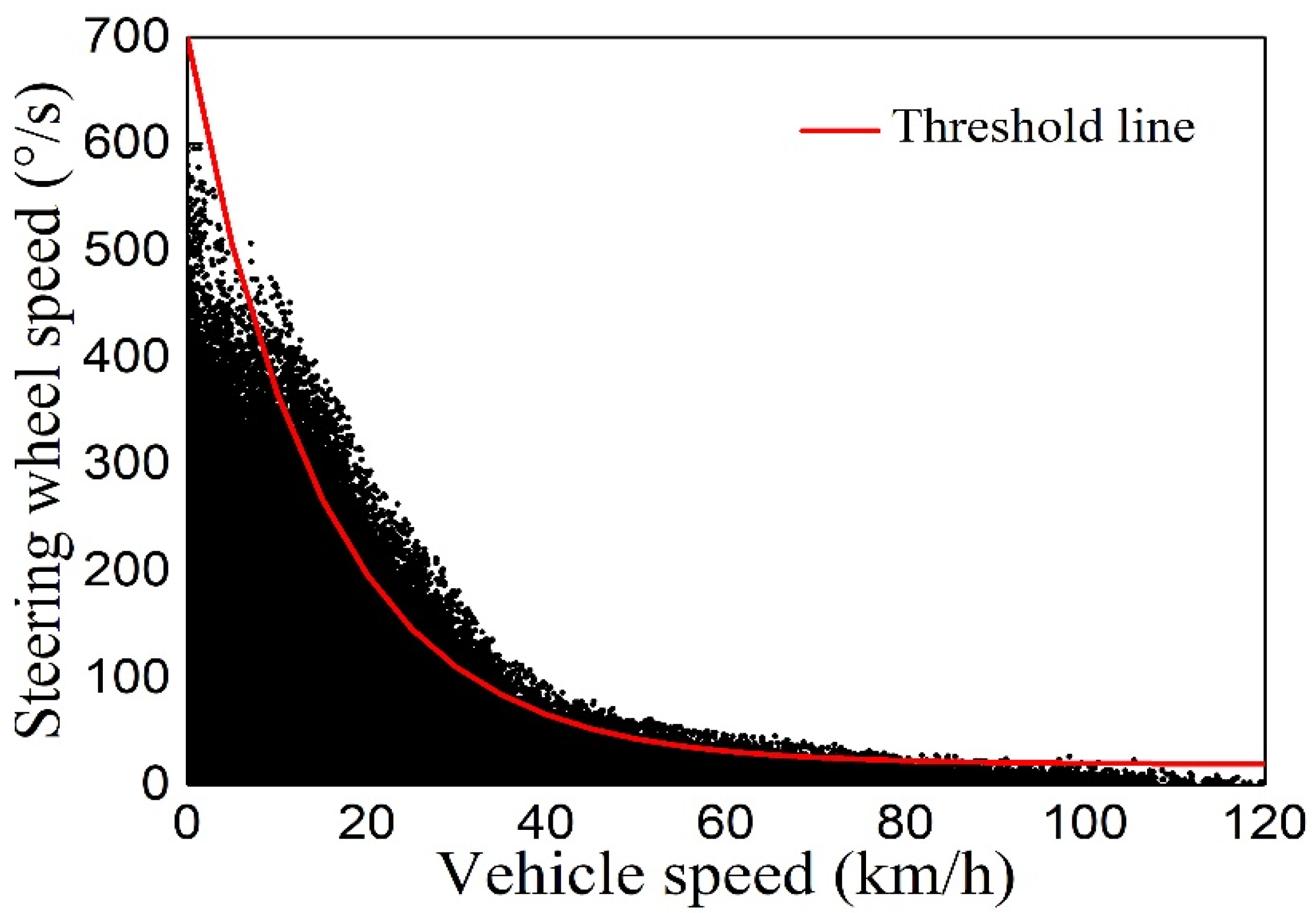
The changing trend of the steering wheel speed was also exponentially fitted with vehicle speed to obtain the threshold of rapid turning. The exponential fitting equation is expressed as Equation (8).
where is vehicle speed and , and are the coefficients of exponential fit. The exponential fit result is shown in Table 5.
Considering the influence of the speed on the safety of steering action, the evaluation of the rapid turning should consider the speed. According to the distribution and quantile of rapid turning, the quantile of 99% was selected as the threshold to distinguish the abnormal steering action, which is shown in Figure 15. The threshold of rapid turning decreased with the increase in vehicle and the setting method of the threshold can distinguish the rapid turning more effectively.
The previous analysis investigated the influence of vehicle speed on driving behaviours, such as acceleration, deceleration and steering action. According to the analysis, the threshold of aberrant driving behaviours were established to identify rapid acceleration, sudden braking, and rapid turning. In the next section, these thresholds were employed to calculate the number of occurrences for aberrant driving behaviour, which can be used to evaluate the driving behaviours.
5. Evaluation Method of Driving Behaviour
5.1. Confirmation of Weight and Scoring Rule
According to the previous analysis, 11 indexes related to driving safety were utilized to evaluate driving behaviour. The evaluation result is influenced by the weight of indexes which can be confirmed by either the subjective or objective evaluation method. Subjective evaluation confirms the weight according to experience. Objective evaluation calculates the weight based on the relationship between the indexes. This study confirmed the weight of indexes by combining the subjective and objective evaluation method.
The comprehensive multi-index evaluation system was composed of two hierarchies. The first layer was the criterion layer, which consisted of three indexes: driving action, vehicle operation and fatigue driving/power consumption. The second layer was the index layer that consisted of the 11 indexes. The detailed index structure is shown in Table 6.
Firstly, the weights of the indexes were preliminarily determined with the Analytic Hierarchy Process (AHP) method, which was a subjective evaluation. According to the experience, the judgement matrix was confirmed and used to indicate the relative importance degree of the indexes in the same layer. Assuming the index number of criterion layer m and the number of index layer n, the weight of indexes for the criterion layer () and index layer () can be calculated by Equation (9).
where and are the product of value in every row of the judgement matrix.
Secondly, the weight was further confirmed by the Entropy Weight Method (EWM), which was an objective evaluation. The EWM confirmed the weight of indexes according to the difference in the samples. Assuming the evaluation objectives are expressed as , the indexes are as follows: , is the original value of the jth index in the ith sample and is the treated value by the Equation (10). The weight of index () can be calculated by EWM method using Equation (11).
where is the weight of the index in the sample and this can be expressed as Equation (12).
Finally, the comprehensive index weight () can be calculated from and using Equation (13). Then, the normalisation can be applied to index layer, which is expressed as . The final weight () can be obtained from the product of and , as shown in Equation (14).
The judgement matrix was established based on the questionnaire introduced in previous studies [31,32,33], as shown in Table 7. The values in the matrix indicated the relative importance degree of the indexes. The final weights () were calculated by combining the AHP and EWM, which were shown in Table 8. It can be seen that the number of speeding occurrences during steering per 100 km had the maximum value of the weight and score. This suggests that the speeding during steering was the most dangerous behaviour among the selected indexes. Other indexes with higher weight or score were also risky in terms of causing traffic accidents.
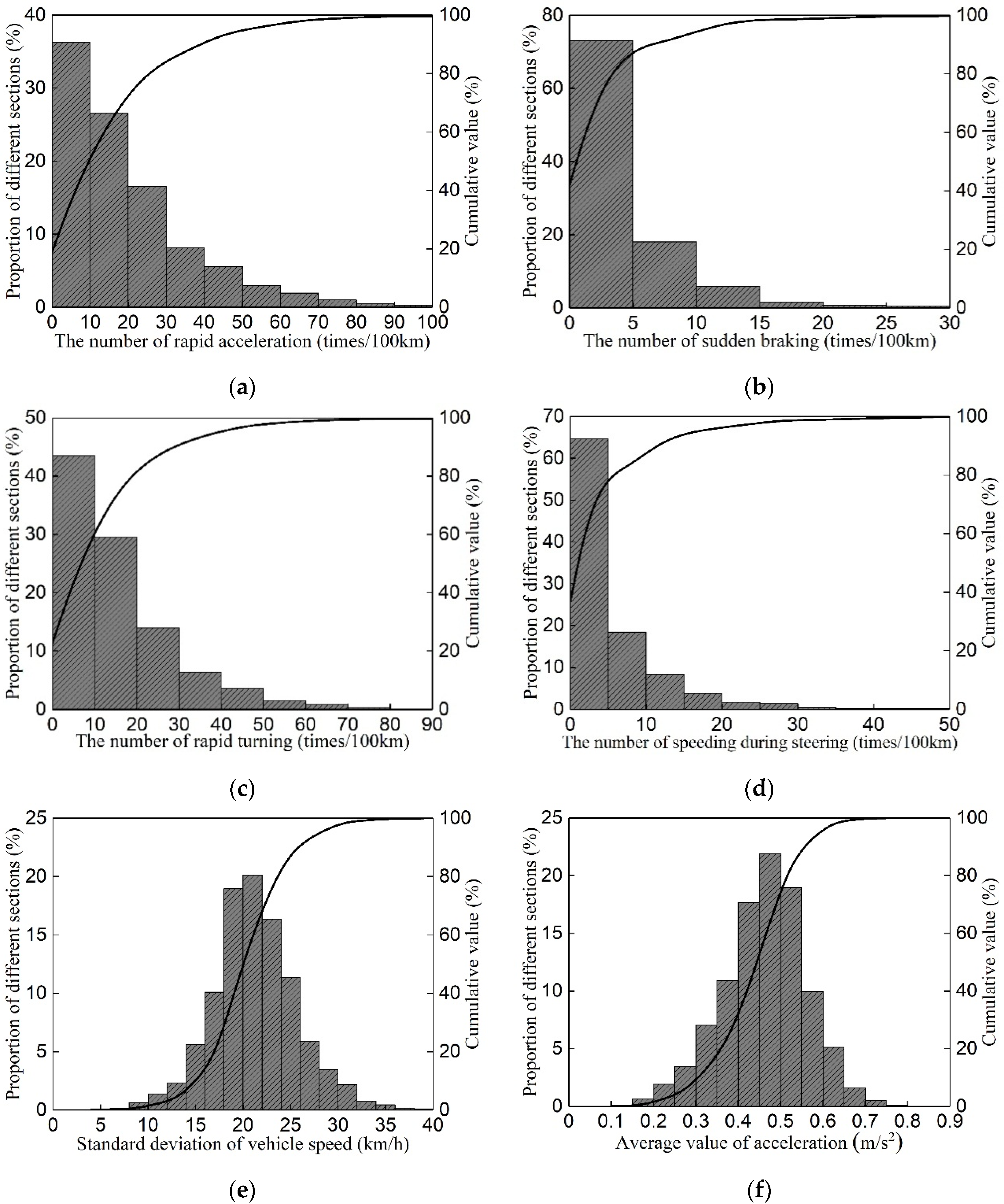
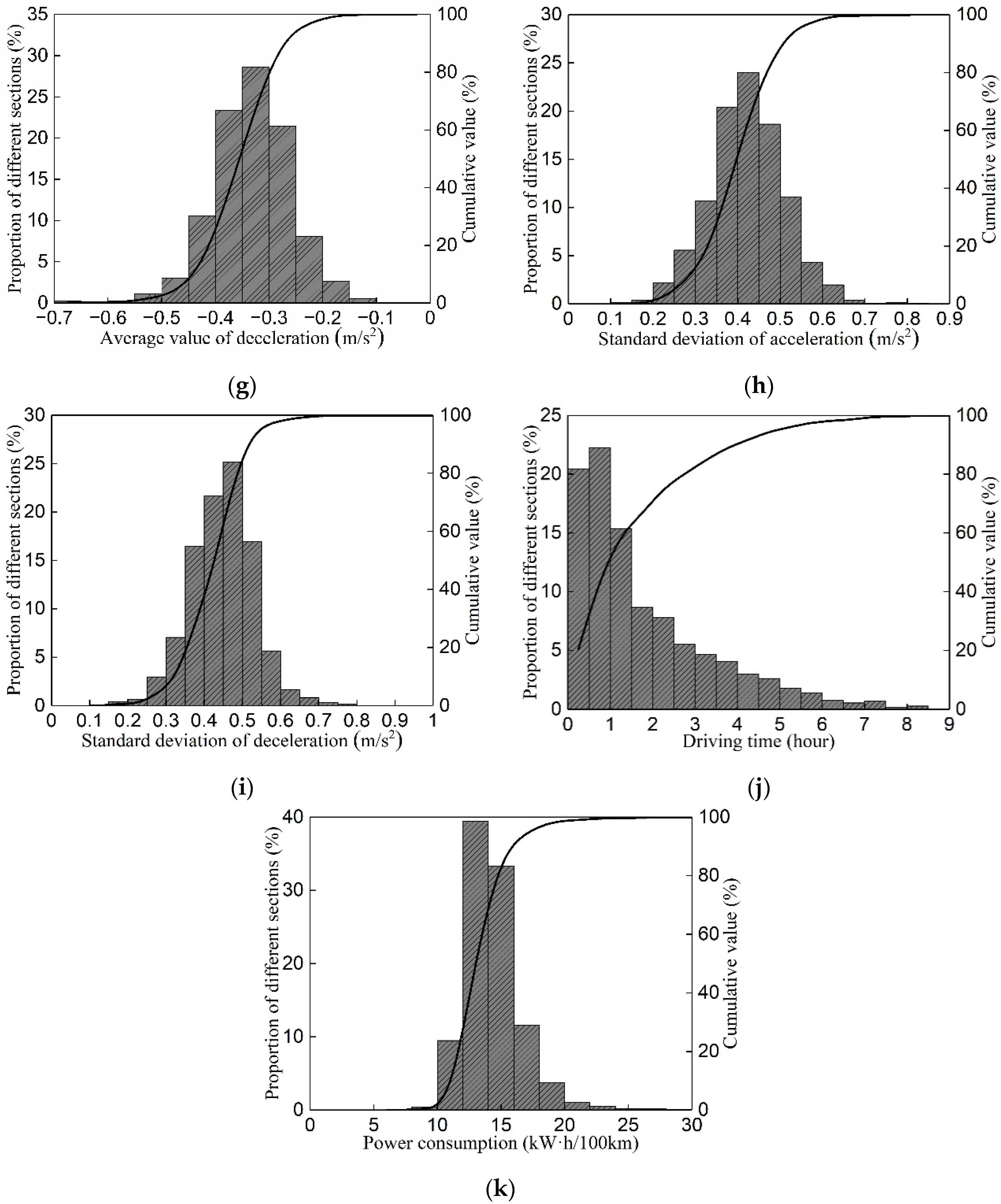
After the confirmation of the index weight, the scoring rule for different indexes was set to accurately evaluate the driving behaviour. The distribution of the 11 indexes was analysed and compared in Figure 16. Figure 16a shows the distribution of the number of rapid accelerations per 100 km. It can be seen that the number gradually decreased and in over 90% of cases, it was lower than 50 times. According to the distribution and the weight of the index, the scoring rule was set with a cut-off point of 50. The other scoring rules of the indexes were confirmed with the similar treatment by combining the distribution and the weight, and the results are shown in Table 9.
5.2. Proposed Driving Behaviour Evaluation Method
Based on the previous analysis, a driving behaviour evaluation method was proposed. This method included driving behaviour data acquisition, data pre−processing, recognition of the aberrant driving behaviour by statistics, index value calculation and output of the score. The flow chart of the evaluation process is shown in Figure 17.
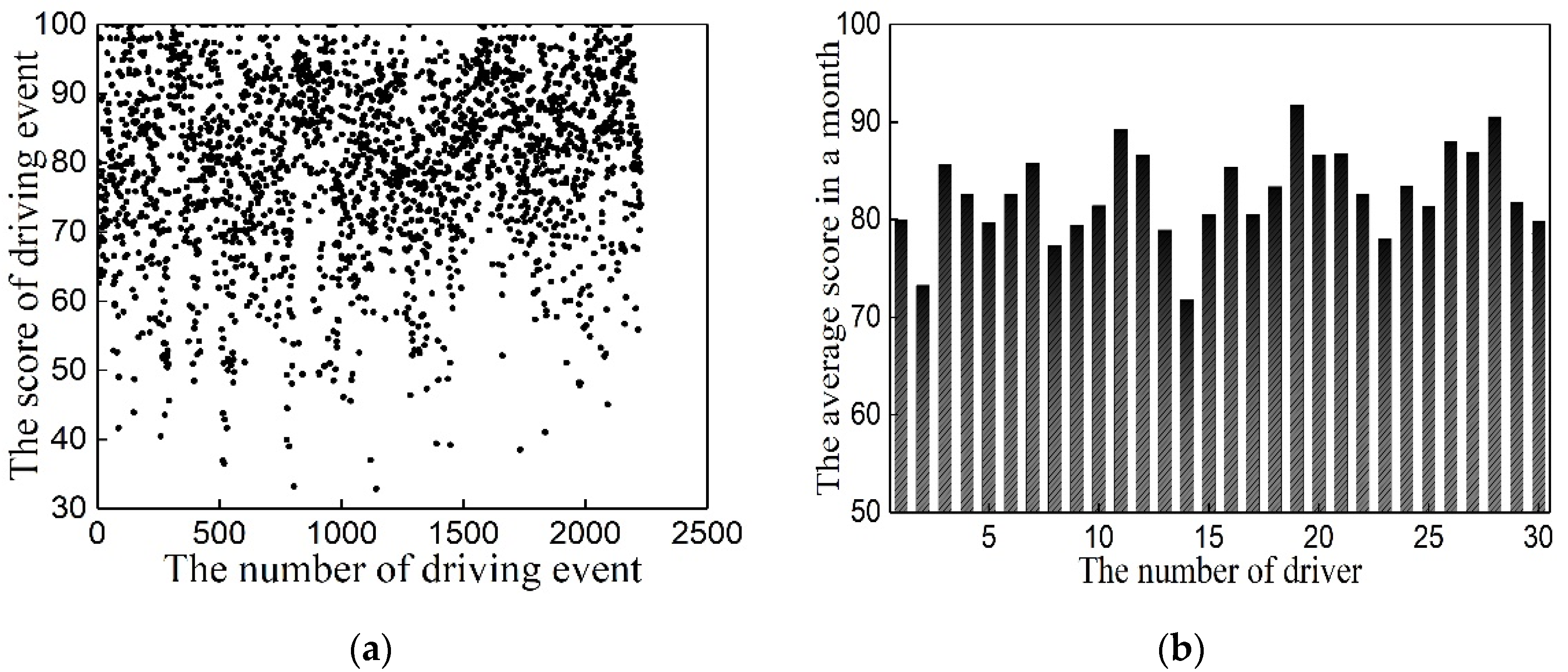
To verify the effectiveness of the evaluation method, thirty drivers were selected from the online car−hiring. The driving behaviour data were selected in one month with 2227 driving events. The scoring result for each driving event was calculated and compared in Figure 18. Most of the scoring results were located from 70 to 100, which indicates that most of the driver behaviours were cautious. There were also some scoring results lower than 60, which can be considered as unsafe driving behaviours. To quantitatively evaluate the driving behaviour of a driver, the average score for every driver in a month was obtained by averaging the score of each driving event, which is shown in Figure 18b. The comparison result showed that the score difference was considerable for each driver. The evaluation result suggested that the scores of the driver number 2 and 14 were relatively low.
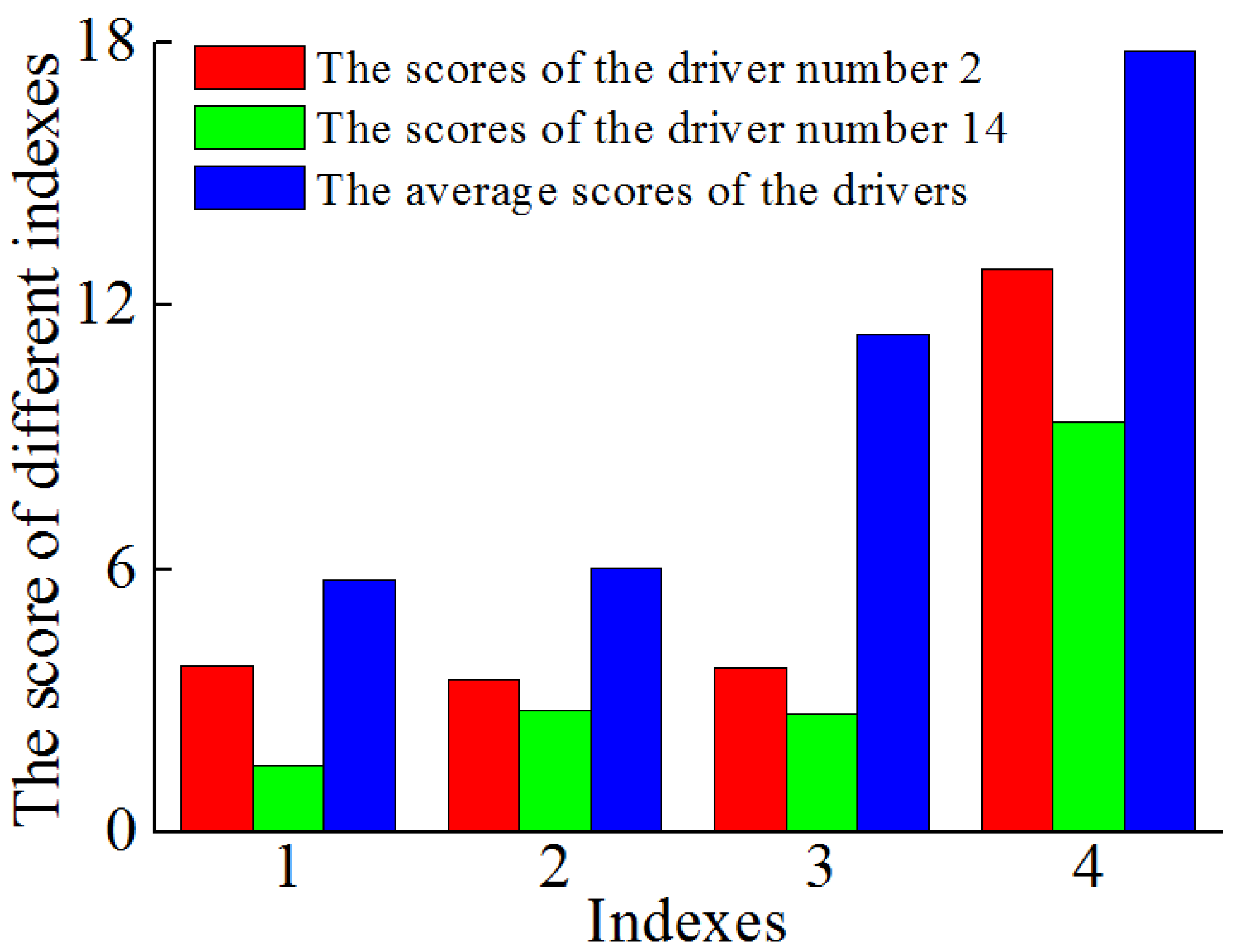
In order to investigate the reasons for the low scores of drivers 2 and 14, the score of the four indexes were compared in Figure 19. The four indexes were the number of rapid accelerations per 100 km, the number of sudden brakings per 100 km, the number of rapid turns per 100 km and the number of speeding occurrences during steering per 100 km, which were closely related with aberrant driving behaviour. The scores of drivers 2 and 14 were also compared with the average scores of the thirty drivers. It can be seen that the scores of the selected four indexes for drivers 2 and 14 were obviously lower than the average scores. Additionally, the score of driver number 14 was lower than that of driver number 2. A lower score meant more aberrant driving behaviour, which showed the effectiveness of the evaluation method. The scoring result can be an important reference for the passenger transport company to distinguish the driver with abnormal or dangerous driving behaviour. The driving behaviour scores can also be an important basis for evaluation for the insurance company to collect the premium.
6. Conclusions
This study proposed a quantitative evaluation method of driving behaviour based on NDS data collected from shared-electrical cars and online car-hiring services. Data acquisition, treatment method and data volume verification were analysed to ensure the effectiveness of the dataset. The distribution characteristics of the main driving behaviour parameters were studied. On this basis, the evaluation method was proposed and verified. The main conclusions were shown as follows. The main differences between the electrical vehicles and vehicles powered by ICE were in the deceleration phase. There was braking energy recovery for the electrical vehicles. Therefore, the conclusion can be basically applied to the ICE vehicles.
- The NDS data were collected from the OBD−II interface via CAN bus with the rate of 10 Hz. This sampling frequency satisfies the requirement of transient process analysis. The sliding-window averaging filter and the box diagram method were used to improve the data quality. Eleven indexes were selected to evaluate the driving behaviour, including vehicle running data, driver operation data and power consumption of the vehicles.
- KL divergence was applied to confirm the appropriate data quantity for the driving behaviour analysis. The result showed that the minimum data quantity for vehicle speed, acceleration, steering wheel angle and steering wheel speed were 20 × 105, 63 × 105, 10 × 105, 231 × 105, respectively, with the variation value of KL lower than 1 × 10⁵.
- The changing trend of acceleration and deceleration, steering wheel angle and steering wheel speed versus vehicle speed were compared. Based on the distribution characteristics, the thresholds of aberrant driving were determined in correlation with vehicle speed to enhance the recognition accuracy of the aberrant driving behaviour. The thresholds can be used to evaluate the aberrant driving behaviour.
- The weights for the 11 indexes were obtained by combining the AHP and EWM methods. The scoring rules of the 11 indexes were confirmed based on the distribution of the indexes. An evaluation method of driving behaviour was proposed and verified according to the driving behaviour data of the car-hiring driver.
In future research, more parameters will be considered including, road slope, weather, driving experience and so on. Additionally, other useful sensors will be used to obtain more driving behaviour parameters. On this basis, the scoring rule will be further optimized and the accuracy of the evaluation method can be subsequently improved.
Author Contributions
Formal analysis, X.L.; methodology, Y.C.; software, K.Z. and S.S.; validation, Z.Y.; writing—original draft, S.J.; writing—review and editing, G.T. All authors have read and agreed to the published version of the manuscript.
Funding
This research was funded by National Key Research and Development Program, grant number 2020YFB1600501; Major Technology Innovation Projects of Shandong Province, grant number 2019TSLH0203; Natural Science Foundation of Shandong Province, grant number ZR2020ME180; National Natural Science Foundation of China, grant number 51976107.
Institutional Review Board Statement
Ethical review and approval were waived for this study due to the reason that the driving behaviour data in this study was obtained from the vehicle operation data and did not involve any personal information, such as GPS data and so on.
Informed Consent Statement
Informed consent was obtained from all subjects involved in the study.
Data Availability Statement
The data were obtained from the OBD−II interface, which only contained the vehicle and components operation data. The driving behaviour data were obtained from the vehicle operation data.
Conflicts of Interest
The authors declare that they have no known competing financial interest or personal relationships that could have appeared to influence the work reported in this paper.
Abbreviations
| AHP | Analytic Hierarchy Process |
| CAN | Controller Area Network |
| ECU | Electronic Control Units |
| EWM | Entropy Weight Method |
| GPS | Global Positioning System |
| ICE | Internal Combustion Engine |
| IMU | Inertial Measurement Unit |
| KL | Kullback–Leibler |
| NDS | Naturalistic Driving Study |
| OBD | On-Board Diagnostics |
References
- Singh, H.; Kathuria, A. Analyzing driver behavior under naturalistic driving conditions: A review. Accid. Anal. Prev. 2021, 150, 105908. [Google Scholar] [CrossRef] [PubMed]
- Singh, S. Critical Reasons for Crashes Investigated in the National Motor Vehicle Crash Causation Survey; National Center for Statistics and Analysis: Washington, DC, USA, 2015.
- Tanvir, S.; Chase, R.T.; Roupahil, N.M. Development and analysis of eco-driving metrics for naturalistic instrumented vehicles. J. Intell. Transp. Syst. 2021, 25, 235–248. [Google Scholar] [CrossRef] [Green Version]
- Ersan, Ö.; Üzümcüoğlu, Y.; Azık, D.; Fındık, G.; Kaçan, B.; Solmazer, G.; Özkan, T.; Lajunen, T.; Öz, B.; Pashkevich, A.; et al. The relationship between self and other in aggressive driving and driver behaviors across countries. Transp. Res. Part F Traffic Psychol. Behav. 2019, 66, 122–138. [Google Scholar] [CrossRef]
- Deng, Z.; Chu, D.; Wu, C.; He, Y.; Cui, J. Curve safe speed model considering driving style based on driver behaviour questionnaire. Transp. Res. Part F Traffic Psychol. Behav. 2019, 65, 536–547. [Google Scholar] [CrossRef]
- Han, H.; Kim, S.; Choi, J.; Park, H.; Yang, J.H.; Kim, J. Driver’s avoidance characteristics to hazardous situations: A driving simulator study. Transp. Res. Part F Traffic Psychol. Behav. 2021, 81, 522–539. [Google Scholar] [CrossRef]
- Papazikou, E.; Thomas, P.; Quddus, M. Developing personalised braking and steering thresholds for driver support systems from SHRP2 NDS data. Accid. Anal. Prev. 2021, 160, 106310. [Google Scholar] [CrossRef]
- Akamatsu, M.; Green, P.; Bengler, K. Automotive technology and human factors research: Past, present, and future. Int. J. Veh. Technol. 2013, 2013, 1–27. [Google Scholar] [CrossRef]
- Precht, L.; Keinath, A.; Krems, J.F. Effects of driving anger on driver behavior—Results from naturalistic driving data. Transp. Res. Part F Traffic Psychol. Behav. 2017, 45, 75–92. [Google Scholar] [CrossRef]
- Ellison, A.B.; Greaves, S.P.; Bliemer, M.C.J. Driver behaviour profiles for road safety analysis. Accid. Anal. Prev. 2015, 76, 118–132. [Google Scholar] [CrossRef]
- Shridhar Bokare, P.; Kumar Maurya, A. Study of effect of speed, acceleration and deceleration of small petrol car on its tail pipe emission. Int. J. Traffic Transp. Eng. 2013, 3, 465–478. [Google Scholar] [CrossRef] [Green Version]
- Sun, Q.; Xia, J.; Nadarajah, N.; Falkmer, T.; Foster, J.; Lee, H. Assessing drivers’ visual-motor coordination using eye tracking, GNSS and GIS: A spatial turn in driving psychology. J. Spat. Sci. 2016, 61, 299–316. [Google Scholar] [CrossRef]
- Sheykhfard, A.; Haghighi, F. Performance analysis of urban drivers encountering pedestrian. Transp. Res. Part F Traffic Psychol. Behav. 2019, 62, 160–174. [Google Scholar] [CrossRef]
- Bokare, P.S.; Maurya, A.K. Acceleration-deceleration behaviour of various vehicle types. Transp. Res. Procedia 2017, 25, 4733–4749. [Google Scholar] [CrossRef]
- Chen, R.; Kusano, K.D.; Gabler, H.C. Driver behavior during overtaking maneuvers from the 100-car naturalistic driving study. Traffic Inj. Prev. 2015, 16, S176–S181. [Google Scholar] [CrossRef]
- Mahapatra, G.; Maurya, A.K. Study of vehicles lateral movement in non-lane discipline traffic stream on a straight road. Procedia Soc. Behav. Sci. 2013, 104, 352–359. [Google Scholar] [CrossRef] [Green Version]
- Papadimitriou, E.; Argyropoulou, A.; Tselentis, D.I.; Yannis, G. Analysis of driver behaviour through smartphone data: The case of mobile phone use while driving. Saf. Sci. 2019, 119, 91–97. [Google Scholar] [CrossRef]
- Saleh, K.; Hossny, M.; Nahavandi, S. Driving behavior classification based on sensor data fusion using LSTM recurrent neural networks. In Proceedings of the 2017 IEEE 20th International Conference on Intelligent Transportation Systems (ITSC), Yokohama, Japan, 16–19 October 2017. [Google Scholar]
- Sangster, J.; Rakha, H.; Du, J. Application of naturalistic driving data to modeling of driver car-following behavior. Transp. Res. Rec. 2013, 2390, 20–33. [Google Scholar] [CrossRef]
- Jachimczyk, B.; Dziak, D.; Czapla, J.; Damps, P.; Kulesza, W. IoT on-board system for driving style assessment. Sensors 2018, 18, 1233. [Google Scholar] [CrossRef] [Green Version]
- Mayhew, D.R.; Simpson, H.M. The safety value of driver education and training. Inj. Prev. J. Int. Soc. Child Adolesc. Inj. Prev. 2002, 8 (Suppl. 2), ii3–ii8. [Google Scholar]
- Zhao, Y.; Yamamoto, T.; Morikawa, T. An analysis on older driver’s driving behavior by GPS tracking data: Road selection, left/right turn, and driving speed. J. Traffic Transp. Eng. 2018, 5, 56–65. [Google Scholar] [CrossRef]
- Feng, F.; Bao, S.; Sayer, J.R.; Flannagan, C.; Manser, M.; Wunderlich, R. Can vehicle longitudinal jerk be used to identify aggressive drivers? An examination using naturalistic driving data. Accid. Anal. Prev. 2017, 104, 125–136. [Google Scholar] [CrossRef] [PubMed]
- Das, A.; Ghasemzadeh, A.; Ahmed, M.M. Analyzing the effect of fog weather conditions on driver lane-keeping performance using the SHRP2 naturalistic driving study data. J. Saf. Res. 2019, 68, 71–80. [Google Scholar] [CrossRef] [PubMed]
- Kong, X.; Das, S.; Jha, K.; Zhang, Y. Understanding speeding behavior from naturalistic driving data: Applying classification based association rule mining. Accid. Anal. Prev. 2020, 144, 105620. [Google Scholar] [CrossRef] [PubMed]
- Morgenstern, T.; Schott, L.; Krems, J.F. Do drivers reduce their speed when texting on highways? A replication study using European naturalistic driving data. Saf. Sci. 2020, 128, 104740. [Google Scholar] [CrossRef]
- Hallmark, S.L.; Tyner, S.; Oneyear, N.; Carney, C.; McGehee, D. Evaluation of driving behavior on rural 2-lane curves using the SHRP 2 naturalistic driving study data. J. Saf. Res. 2015, 54, 17.e1–27. [Google Scholar] [CrossRef] [Green Version]
- Ji, S.; Chen, Q.; Shu, M.; Tian, G.; Liao, B.; Lv, C.; Li, M.; Lan, X.; Cheng, Y. Influence of operation management on fuel consumption of coach fleet. Energy 2020, 203, 117853. [Google Scholar] [CrossRef]
- Sagberg, F.; Selpi; Bianchi Piccinini, G.F.; Engström, J. A review of research on driving styles and road safety. Hum. Factors 2015, 57, 1248–1275. [Google Scholar] [CrossRef]
- Wang, W.; Liu, C.; Zhao, D. How much data is enough? A statistical approach with case study on longitudinal driving behavior. IEEE Trans. Intell. Veh. 2017, 2, 85–98. [Google Scholar] [CrossRef] [Green Version]
- Wang, Z. Research on Vehicle Insurance Pricing Based on UBI Driving Behaviour Score. Master’s Thesis, Hunan University, Hunan, China, 2019. [Google Scholar]
- Peng, J. Research on Usage-Based Insurance Premiums and Driving Behaviour Scoring Based on GID. Master’s Thesis, Nanjing University of Posts and Telecommunications, Nanjing, China, 2016. [Google Scholar]
- Tselentis, D.I.; Yannis, G.; Vlahogianni, E.I. Innovative motor insurance schemes: A review of current practices and emerging challenges. Accid. Anal. Prev. 2017, 98, 139–148. [Google Scholar] [CrossRef]
Figure 1.
The main study flow chart.

Figure 2.
The acquisition process of the NDS data.

Figure 3.
The vehicle speed versus time in a complete driving event.

Figure 4.
The comparison of the signal with different treat method: (a) Sliding-window averaging filter; (b) The box diagram method.
Figure 4.
The comparison of the signal with different treat method: (a) Sliding-window averaging filter; (b) The box diagram method.

Figure 5.
The KL of different parameters versus data quantity.

Figure 6.
The distribution characteristic of the vehicle speed.

Figure 7.
The distribution characteristic of acceleration and deceleration.

Figure 8.
The distribution characteristic of steering wheel angle.

Figure 9.
The distribution characteristic of steering wheel speed.

Figure 10.
The distribution characteristic of acceleration and deceleration versus vehicle speed: (a) Overall trend; (b) Comparison of distribution characteristic.
Figure 10.
The distribution characteristic of acceleration and deceleration versus vehicle speed: (a) Overall trend; (b) Comparison of distribution characteristic.

Figure 11.
The comparison of different quantile value for acceleration and deceleration.

Figure 12.
The linear result of quantile for acceleration and deceleration.

Figure 13.
The comparison of distribution and quantile for steering wheel angle at different speeds.
Figure 13.
The comparison of distribution and quantile for steering wheel angle at different speeds.

Figure 14.
The comparison of distribution and quantile for steering wheel speed at different speeds.
Figure 14.
The comparison of distribution and quantile for steering wheel speed at different speeds.

Figure 15.
The distribution of steering wheel speed and threshold of abnormal steering action.

Figure 16.
The distribution of different indexes: (a) The number of rapid accelerations per 100 km; (b) The number of sudden brakings per 100 km; (c) The number of rapid turns per 100 km; (d) The number of speeding occurences during steering per 100 km; (e) Standard deviation of vehicle speed; (f) Average value of acceleration; (g) Standard deviation of acceleration; (h) Average value of deceleration; (i) Standard deviation of deceleration; (j) Driving time per trip; (k) Power consumption.


Figure 17.
The evaluation flow chart of driving behaviour.

Figure 18.
The evaluation result of driving behaviour: (a) The score distribution of driving events; (b) The score for every driver.
Figure 18.
The evaluation result of driving behaviour: (a) The score distribution of driving events; (b) The score for every driver.

Figure 19.
The comparison of scores for four indexes (numbers from 1 to 4 represent the number of rapid accelerations per 100 km, the number of sudden brakings per 100 km, the number of rapid turns per 100 km and the number of speeding occurrences during steering per 100 km, respectively).
Figure 19.
The comparison of scores for four indexes (numbers from 1 to 4 represent the number of rapid accelerations per 100 km, the number of sudden brakings per 100 km, the number of rapid turns per 100 km and the number of speeding occurrences during steering per 100 km, respectively).


Table 1.
The primary parameters collected by the data acquisition system.
| Signal Type | The Primary Parameters |
|---|---|
| Vehicle operation | Vehicle speed, mileage, position of the acceleration and brake pedal, steering wheel angle. |
| Power battery status | Total voltage and current of the battery pack, insulation resistance and temperature. |
| Motor operation | Voltage, current, motor speed, motor torque and temperature. |
| Vehicle accessories status | Voltage and current of the air conditioner, Voltage and current of the DC-DC. |
| Vehicle alert | Alert signal of power battery, motor and thermal management system. |
Table 2.
The indexes used to evaluate the driving behaviour.
| Number | Index | Symbol | Definition | Unit |
|---|---|---|---|---|
| 1 | Standard deviation of vehicle speed | km/h | ||
| 2 | Average value of acceleration | m/s2 | ||
| 3 | Average value of deceleration | m/s2 | ||
| 4 | Standard deviation of acceleration | m/s2 | ||
| 5 | Standard deviation of deceleration | m/s2 | ||
| 6 | The number of rapid acceleration per 100 km | times/100 km | ||
| 7 | The number of sudden braking per 100 km | times/100 km | ||
| 8 | The number of rapid turning per 100 km | times/100 km | ||
| 9 | The number of speeding during steering per 100 km | times/100 km | ||
| 10 | Driving time per trip | - | hour | |
| 11 | Power consumption per 100 km | kW·h/100 km |
where i is the number of sample point, n is the total number of sample point in a complete driving event, vi is the vehicle speed of each sample point, vm is the average speed in a complete driving event, is the acceleration of each sample point, is the deceleration of each sample point, Na, Nd, Nt and Nst are the number of occurrences of rapid acceleration, sudden braking, rapid turning and speeding during steering, respectively, in a complete driving event, D is the mileage in a complete driving event, and W is the power consumption in a complete driving event.
Table 3.
The linear fit result of the acceleration.
| Coefficient | 50% | 85% | 90% | 95% | 99% | 99.9% |
|---|---|---|---|---|---|---|
| β1 | −0.0042 | −0.0090 | −0.0102 | −0.0118 | −0.0150 | −0.0238 |
| β2 | 0.5312 | 1.2056 | 1.4002 | 1.7076 | 2.5000 | 3.5534 |
| R2 | 0.9123 | 0.9351 | 0.9386 | 0.9477 | 0.9708 | 0.9930 |
Table 4.
The linear fit result of the deceleration.
| Coefficient | 50% | 85% | 90% | 95% | 99% | 99.9% |
|---|---|---|---|---|---|---|
| β1 | −0.0087 | −0.0128 | −0.0146 | −0.0182 | −0.030 | −0.0565 |
| β2 | −0.2903 | −0.8529 | −1.0147 | −1.2648 | −1.8500 | −2.6433 |
| β3 | 0.0047 | 0.0105 | 0.012 | 0.0144 | 0.0220 | 0.0301 |
| β4 | −0.5456 | −1.3544 | −1.5801 | −1.9741 | −3.150 | −4.57 |
| R2 | 0.8266 | 0.8263 | 0.8402 | 0.8838 | 0.9494 | 0.9220 |
Table 5.
The exponential fit result of the steering wheel speed.
| Coefficient | 50% | 85% | 90% | 95% | 99% | 99.9% |
|---|---|---|---|---|---|---|
| a | 0.97 | 5.82 | 7.64 | 9.83 | 19.56 | 3.80 |
| b | −53.27 | −209.30 | −270.77 | −373.06 | −680.00 | −692.02 |
| c | 0.948 | 0.940 | 0.936 | 0.936 | 0.935 | 0.949 |
| R2 | 0.9932 | 0.9982 | 0.9985 | 0.9985 | 0.9942 | 0.9935 |
Table 6.
The detailed index structure of driving behaviour evaluation.
| Criterion Layer | Index Layer | Symbol of the Index |
|---|---|---|
| vehicle operation | The number of rapid accelerations per 100 km | |
| The number of sudden brakings per 100 km | ||
| The number of rapid turns per 100 km | ||
| The number of speeding occurrences during steering per 100 km | ||
| driving action | Standard deviation of vehicle speed | |
| Average value of acceleration | ||
| Average value of deceleration | ||
| Standard deviation of acceleration | ||
| Standard deviation of deceleration | ||
| fatigue driving/power consumption | Time of a driving event | |
| Power consumption per 100 km |
Table 7.
The judgement matrix for evaluation of the driving behaviour.
| Criterion Layer | Index Layer |
|---|---|
Table 8.
The final weight for different indexes.
| Index | Weight (Wj) | Value (Percentage) |
|---|---|---|
| The number of rapid accelerations per 100 km | 0.0858 | 9 |
| The number of sudden brakings per 100 km | 0.0677 | 7 |
| The number of rapid turns per 100 km | 0.1580 | 16 |
| The number of speeding occurrences during steering per 100 km | 0.2280 | 22 |
| Standard deviation of vehicle speed | 0.0428 | 4 |
| Average value of acceleration | 0.0233 | 2 |
| Average value of deceleration | 0.0206 | 2 |
| Standard deviation of acceleration | 0.0434 | 4 |
| Standard deviation of deceleration | 0.0333 | 4 |
| Driving time per trip | 0.1525 | 15 |
| Power consumption per 100 km | 0.1445 | 15 |
Table 9.
The scoring rule of different indexes.
| Index | Unit | Score | Score Rule |
|---|---|---|---|
| The number of rapid acceleration per 100 km | times/100 km | 9 | |
| The number of sudden braking per 100 km | times/100 km | 7 | |
| The number of rapid turning per 100 km | times/100 km | 16 | |
| The number of speeding during steering per 100 km | times/100 km | 22 | |
| Standard deviation of vehicle speed | km/h | 4 | |
| Average value of acceleration | m/s2 | 2 | |
| Standard deviation of acceleration | m/s2 | 4 | |
| Average value of deceleration | m/s2 | 2 | |
| Standard deviation of deceleration | m/s2 | 4 | |
| Driving time per trip | hour | 15 | |
| Power consumption | kW·h/100 km | 15 |
Publisher’s Note: MDPI stays neutral with regard to jurisdictional claims in published maps and institutional affiliations. |
© 2022 by the authors. Licensee MDPI, Basel, Switzerland. This article is an open access article distributed under the terms and conditions of the Creative Commons Attribution (CC BY) license (https://creativecommons.org/licenses/by/4.0/).
Share and Cite
MDPI and ACS Style
Ji, S.; Zhang, K.; Tian, G.; Yu, Z.; Lan, X.; Su, S.; Cheng, Y. Evaluation Method of Naturalistic Driving Behaviour for Shared-Electrical Car. Energies 2022, 15, 4625. https://doi.org/10.3390/en15134625
AMA Style
Ji S, Zhang K, Tian G, Yu Z, Lan X, Su S, Cheng Y. Evaluation Method of Naturalistic Driving Behaviour for Shared-Electrical Car. Energies. 2022; 15(13):4625. https://doi.org/10.3390/en15134625
Chicago/Turabian StyleJi, Shaobo, Ke Zhang, Guohong Tian, Zeting Yu, Xin Lan, Shibin Su, and Yong Cheng. 2022. "Evaluation Method of Naturalistic Driving Behaviour for Shared-Electrical Car" Energies 15, no. 13: 4625. https://doi.org/10.3390/en15134625
Note that from the first issue of 2016, this journal uses article numbers instead of page numbers. See further details here.