
Development of a Novel Experimental Facility to Assess Heating Systems’ Behaviour in Buildings
by
 , , and
Wirich Freppel
1,2 ,
,
Geoffrey Promis
1,*,
Anh Dung Tran Le
1,
Omar Douzane
1 and
Thierry Langlet
1 1
Laboratory of Innovative Technologies (EA3899), University of Picardie Jules Verne, Avenue des Facultés—Le Bailly, CEDEX, 80025 Amiens, France
2
Noirot, Groupe Muller, 8 Rue Ampère, CEDEX 02, 02000 Laon, France
*
Author to whom correspondence should be addressed.
Energies 2022, 15(13), 4615; https://doi.org/10.3390/en15134615
Submission received: 7 May 2022
/
Revised: 31 May 2022
/
Accepted: 20 June 2022
/
Published: 23 June 2022
(This article belongs to the Special Issue The Effects of Predictive Control on Energy Performance of Buildings)
Abstract
:The building sector represents approximately 40% of the global energy consumption, of which 18 to 73% is represented by heating and ventilation. One focus of research for reducing energy consumption is to study the interaction between the heating system, the occupant’s behaviour, and the building’s thermal mass. For this purpose, a new experimental facility was developed. It consists of a real accommodation in which the thermal performance of the envelope, the heating system, the room’s layout, the weather conditions, and the occupant’s activity are variable parameters. A simulation model of the experimental facility, built in TRNSYS, was used to characterise the experimental facility. This article details the development of the experimental facility and then compares results for two different types of building inertia (low and high thermal masses). Results show the accuracy of the thermal inertia reproduction in the experimental facility and highlight the possibilities of improvements in the interaction between heating systems and building envelope efficiency.
1. Introduction
Energy efficiency in buildings has been a major environmental preoccupation for a long time now. From the Grenelle Environment Roundtable in 2007 to the conference of Parties in 2021 [1], which gathered local governments, employer organizations, NGOs, and representatives of the central governments, many decisions were made in order to improve energy efficiency in buildings. Firstly, new buildings must reach high levels of insulation as recommended by labels such as BREEAM for England, LEED for the United States of America, and EFFINERGIE for France. Secondly, new strategies for heating and cooling were developed in order to use energy more efficiently [1,2].
Today, the figures show a quite significant improvement in energy efficiency, but more efforts are required to keep the human environmental impact under the threshold that was set up by the United Nations. Looking at the charts from 2017 [3], the building sector represented 40% of the global energy consumption in the world. It was mostly characterized by heating and cooling with a rate between 18 to 73%, depending on the region [4]. For many years, engineers focused on thermal insulation [5,6] and sustainable architecture [7]. However, only 1% of the existing housing stock is renovated every year, and the rate of new construction is less than 1%. It would take at least half a century to replace all the existing stock with high insulated buildings. So the building sector must be observed from another angle in order to optimize its energy consumption.
Usually, the heating system in buildings is used as an additional tool to achieve thermal comfort. However, although very effective when tested individually and in a standard situation, it is still designed to react to physical phenomena that have already occurred. More specifically, the heaters only operate as a function of the indoor air temperature. As this information is the result of the weather conditions and the building’s thermal behaviour, there is generally a gap between the requirements for thermal comfort and the heaters’ reaction. So that, most of the time, the occupants feel either too cold or too warm. This lack of anticipation often results in wasted energy and discomfort. Understanding the relationship between the building and the heating system means the ability to adapt to comfort requirements, and thus more efficiently reduce energy consumption [8,9].
But how do we accurately assess that relationship? To date, most numerical tools are efficient when estimating the energy demand for heating [10], but they are not that efficient for estimating thermal comfort in a variable state. For example, in simulation, occupants are most often considered as a simple energy supply, while in reality, their activities lead to air motions affecting the energy consumption and thermal comfort (e.g., openings, kitchen hood) [11]. In addition, heat transfer from the heating devices is relatively complex and its behaviour is difficult to simulate. For both examples, a Computational Fluid Dynamics (CFD) solver would be needed, in which computing in a building would be time and cost consuming, and difficult to develop. Tian suggested applying CFD to the zone of study while the others are modelled with a simple thermal simulation tool [12]. This solution does not work well when multiple zones interact. An ideal solution would be to combine simulation and experimentation with a real test building that respects several conditions. Firstly, the envelop composition should be quickly variable without the need to change the materials between each test. Secondly, the weather conditions should be also variable and controlled dynamically. Finally, the heating system should be replaceable to study different technologies. In that test building, it would be easy to observe the behaviour of the heating system as a function of the building envelope and weather conditions in a quite fast manner. This paper aims to describe the conception and the validation of an experimental facility in which the building envelop can be changed without affecting the external structure or its geometry and in which weather conditions, the heating system, the thermal response of the envelope, and the occupant’s way of life are controlled. Its aim is to better analyze the interactions between the heating system, the building’s envelope, and the weather conditions.
In experimentation, it is common to use twin houses [13] or a group of several houses with the same design but different envelope compositions [14]. However, they proved their efficiency to highlight the performance of the building but not of the heating system itself. One first problem is the difficulty to meet repeatability with weather conditions since those experimental setups are placed outside. It also enables to study the heating system only during the cold season, which can be rather problematic for fast development. Another problem is the poor number of available envelope compositions, or in other words, the building’s thermal masses, that can be tested. Sun & al. built twelve identical one-node experimental rooms placed in a climatic chamber [15]. Each room had a different envelope composition so that different time lags and decrement factors could be tested. However, those experimental rooms are too small to study thermal transfer between the heating system and the building’s envelope in a real environment. This kind of strategy quickly reaches its limit since the stock of buildings is composed of a large range of different types of architecture [16]. It would be costly and time-intensive to build a new house for each envelope composition to be tested.
For this purpose, a 140 square meter experimental facility was developed. In this facility, most of the influent parameters on thermal exchanges in buildings are controlled without changing their structure. It enables us to observe and study the behaviour of the heating system as if it was placed in a real accommodation under real weather conditions. It was developed following two main features: air exchanges through ventilation and openings and thermal transfer through the envelope. The method used to respect each feature is described in this paper.
A simulation model of the experimental facility was developed using TRNSYS 17 to validate and optimize the experimental facility’s behaviour. A quick description of the model is made in the third section.
2. Description of the Experimental Facility
2.1. Structure and Composition
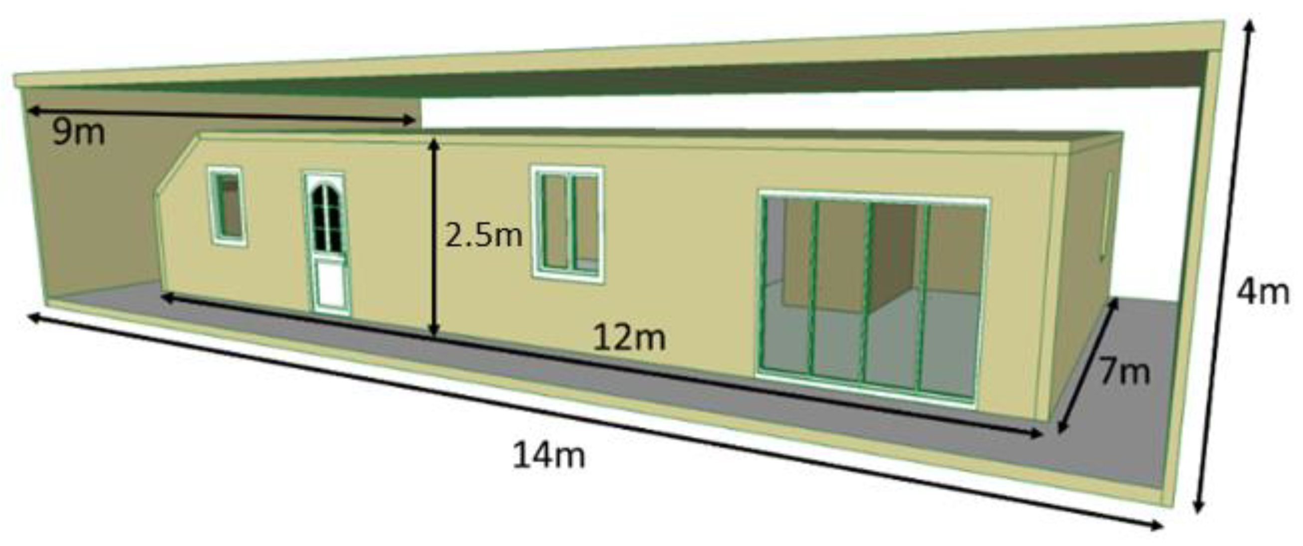
The experimental facility was built to vary its thermal mass and weather conditions without the need to change its structure. In this regard, two enclosures that fit together were built, as shown in Figure 1.
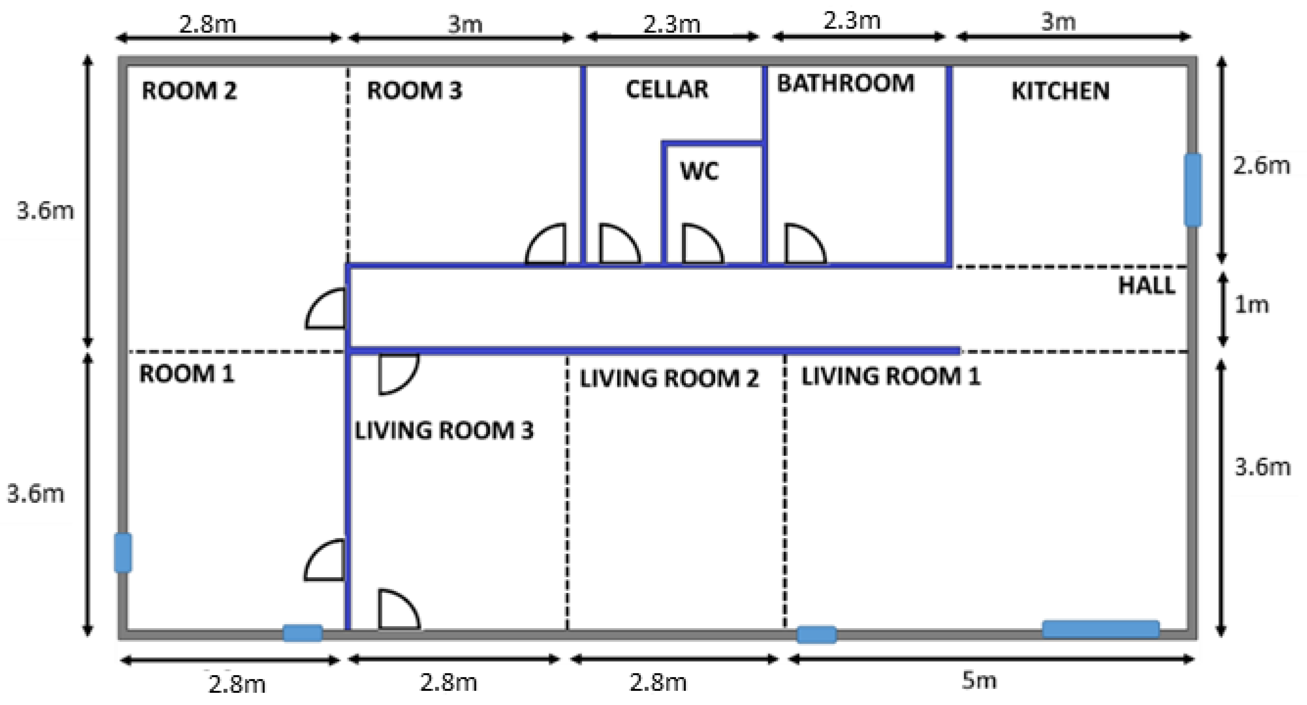
The smaller enclosure represents the accommodation which is called the “test chamber”. This study was carried out with a French industrial partner who wishes to be as close as possible to the existing building heritage in France for the refurbishment market. A preliminary study was carried out to identify the average housing in France. The test chamber, which is based on this study, has an area of 100 m2 and is composed of a kitchen, a living room, several bedrooms, a bathroom, a hall, a toilet, and a utility room (Figure 2). However, in order to extend the study to other housing types, the bedrooms and the living room are equipped with removable walls (dotted lines in Figure 2), which allow to vary the shape and volumes of each room.
The volume between both enclosures is called a “cold chamber”. The bigger enclosure is used as protection from the laboratory thermal contributions and to delimiter the cold chamber. It is made of metallic panels filled with 120 mm thick mineral wool to reduce as much as possible thermal transfer with the laboratory.
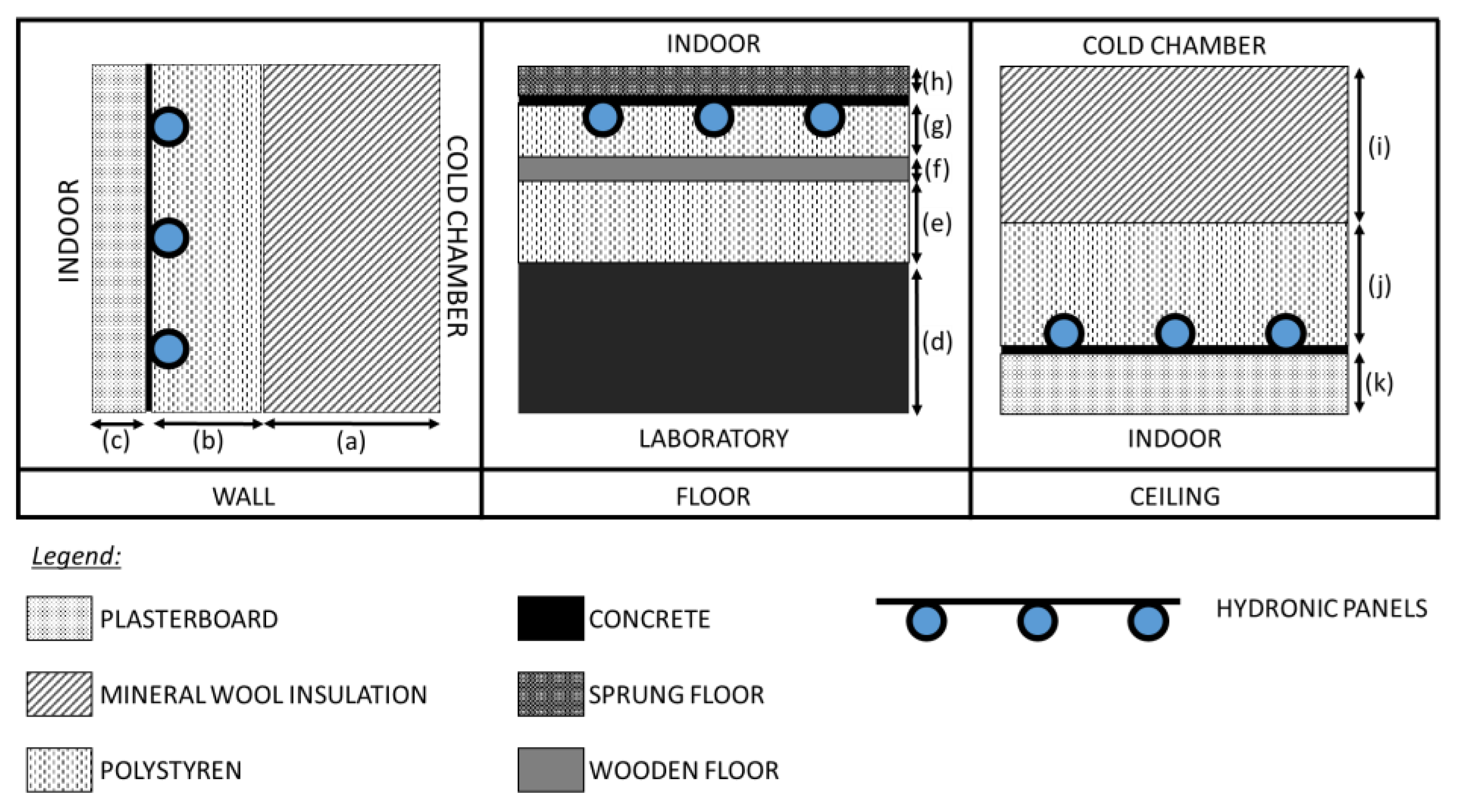
Figure 3 shows the envelope composition of the test chamber. The walls are composed, from outside to inside, of 120 mm thick mineral wool (a), hydronic circuits which were embedded in 30 mm thick polystyrene (b), and a 13 mm thick white painted plasterboard (c). The floor is composed of 160 mm thick concrete (d), 90 mm thick expanded polystyrene (e), a 19 mm thick wooden floor (f), the hydronic circuits embedded in 30 mm thick polystyrene (g), and finally a 10 mm thick sprung floor (h). The ceiling has the same composition as the walls, from the indoor to the cold chamber: a 13 mm-thick white painted plasterboard (k), the hydronic circuits embedded in a 30 mm-thick polystyrene panel (j) and a 120 mm-thick mineral wool layer (i). The thermal resistance of walls and the ceiling is equal to 3.71 m2 K/W, and the floor thermal resistance is equal to 3.60 m2 K/W.
The hydronic circuits were placed all around the envelope of the test chamber, on its inner surface, right behind the plasterboards for walls and ceiling, and under the wooden floor. They can be considered as thermally active panels (TAP), in which the temperature is adapted as a function of time. Section 2.3 is dedicated to detailing the development of this technological solution.
2.2. Thermal Transfer through Ventilation and Openings
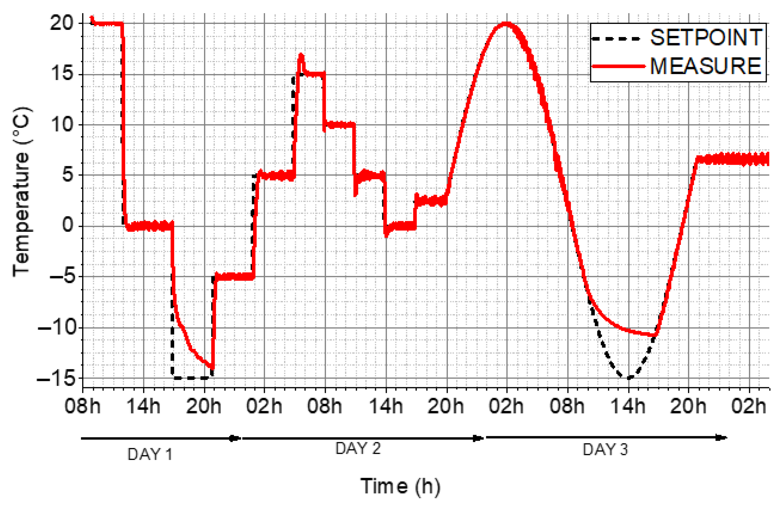
The air in the cold chamber is temperature-controlled and represents a volume of about 300 m3. Its aim is to reproduce thermal transfer through openings and ventilation as if the test chamber was located outside. Three heat exchangers are placed in the cold chamber, having a total cooling and heating power of 17 kW which enable to vary the air temperature to high reactivity, as shown in Figure 4. The power is such that it can decrease the air temperature by 3 °C per minute and increase it by the same rate. This is much more than needed for a north European climate.
As shown in Figure 4, a typical daily evolution of the outside air temperature was applied at the end of day 2. The positive part was well respected, unlike the negative part where the set point of −10 °C was hardly reached. According to this result, the outside air temperature was set as a variable from −10 °C to +20 °C. As a reminder, this work focuses on studying the heating system’s behaviour, so it is not necessary to reach a higher temperature than 20 °C in the cold chamber.
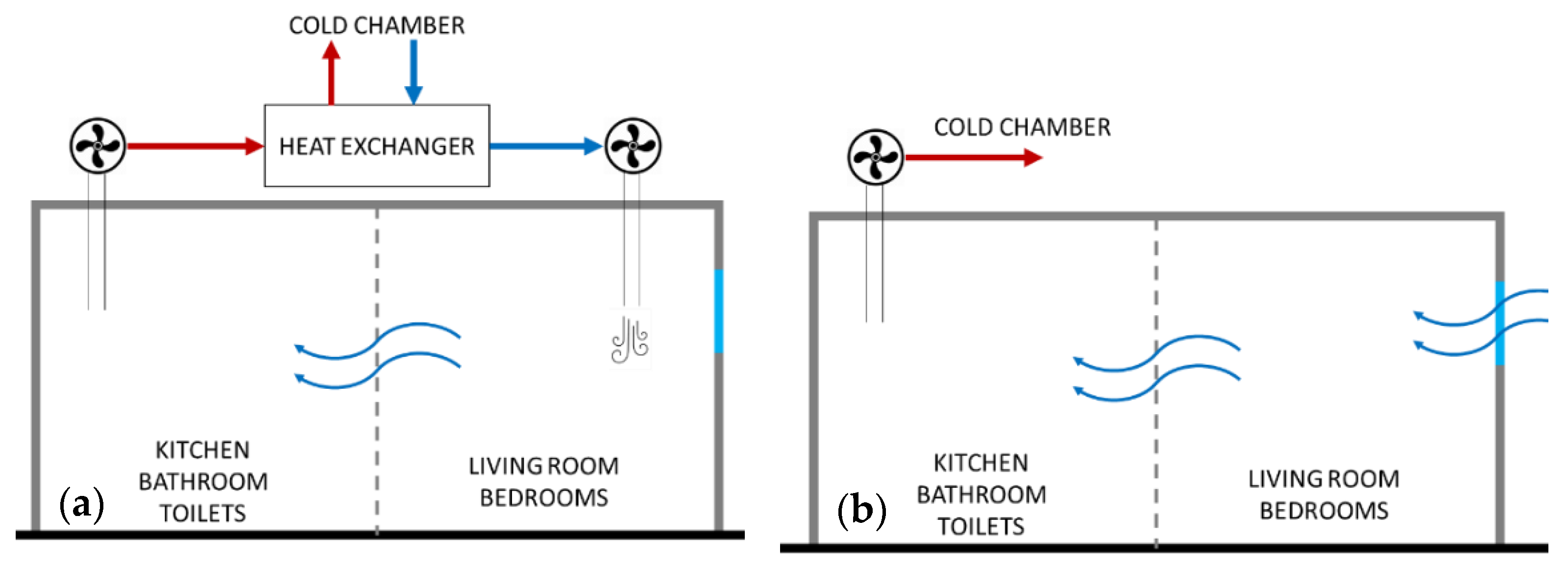
Two ventilation networks were installed in the test chamber: exhaust air ducts and fresh air ducts. Two configurations of these networks are possible:
When the dual flow ventilation system is used, inlets from the windows are closed. The dual flow ventilation engine can be replaced by any ventilation solution. The purpose here is to be able to compare dual flow engines in terms of energy efficiency and also in terms of indoor air quality.
2.3. Thermal Transfer through the Envelope
The TAPs were placed all around the test chamber’s envelope, on its inner surface to control the thermal response of the external walls regarding the environmental solicitations. The objective, by using TAPs, is to control the temperature of the envelope as a function of time.
2.3.1. Control of the Thermally Active Panels
Looking at the thermal balance of inner and outer surfaces of a wall, heat transfer depends on multiple factors such as weather conditions, the wall’s composition, and indoor conditions. The thermal balance on the inner surface shows that its temperature can, only by itself, represent results from all the heat fluxes which occur on the envelope at each time step [8,17]. That means, by continuously controlling the inner surface temperature of the envelope, it is possible to simulate specific weather conditions and envelop composition. This is the purpose of the TAPs.
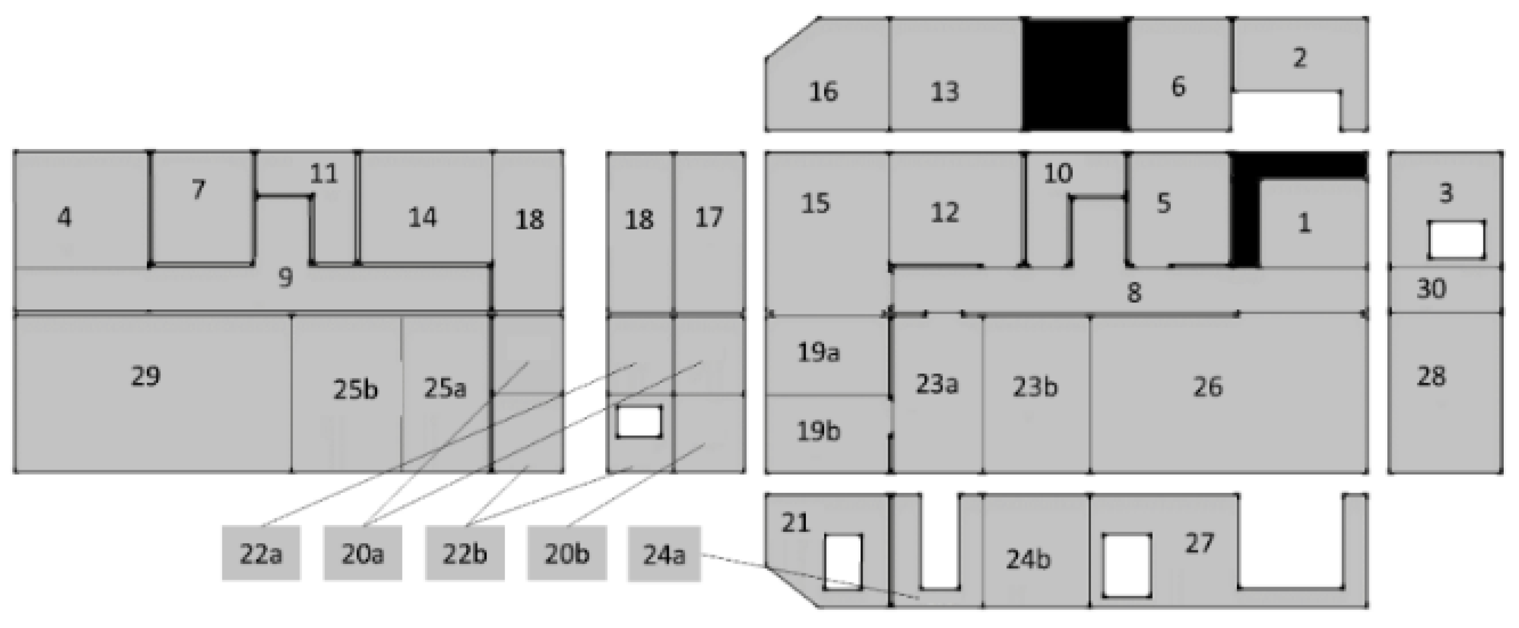
The entire surface of the TAPs was divided into 36 thermally independent ones. Figure 6 shows the cutting of the envelope, all surfaces are illustrated on a plan. This setup is necessary since the thermal behaviour of the envelope is not homogenous. For example, two adjacent walls that are exposed to the same outdoor conditions, but different indoor conditions, would present different temperatures on their surface. So one TAP is associated with one surface of the envelope only.
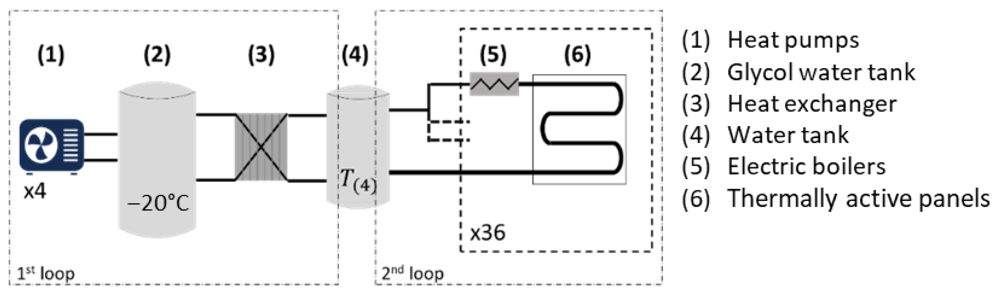
The thermal regulation of each TAP is provided by two thermal loops (Figure 7), the first one is the refrigerant loop, and the second one is the heating loop. In the first loop, four heat pumps (1) keep the temperature of a 1500 L glycol water tank (2) at −20 °C. A 700 L water tank (4) is linked to (2) by a plate heat exchanger (3). The first loop is common to all TAPs; thus, the outlet temperature of the water tank is equal to the lowest inner surface temperature to reach among the 36 ones (w = [1:36]), to which we substrate two more degrees in order to allow quick cooling of the walls if needed, as shown in Equation (1). This setting is updated at each time step.
The second loop is used to heat the water flowing to the TAPs. The cold water from (4) is pumped and sent to 36 electric boilers (5). Each one is linked to a TAP (6) and heats the entering water following a PI regulation loop. There is no set point to reach in the water as the real set point is located on the surface of the wall, ceiling, or floor. So here we have an open-loop control. The heaters are switched on and off in order to reach the target temperature at the surface.
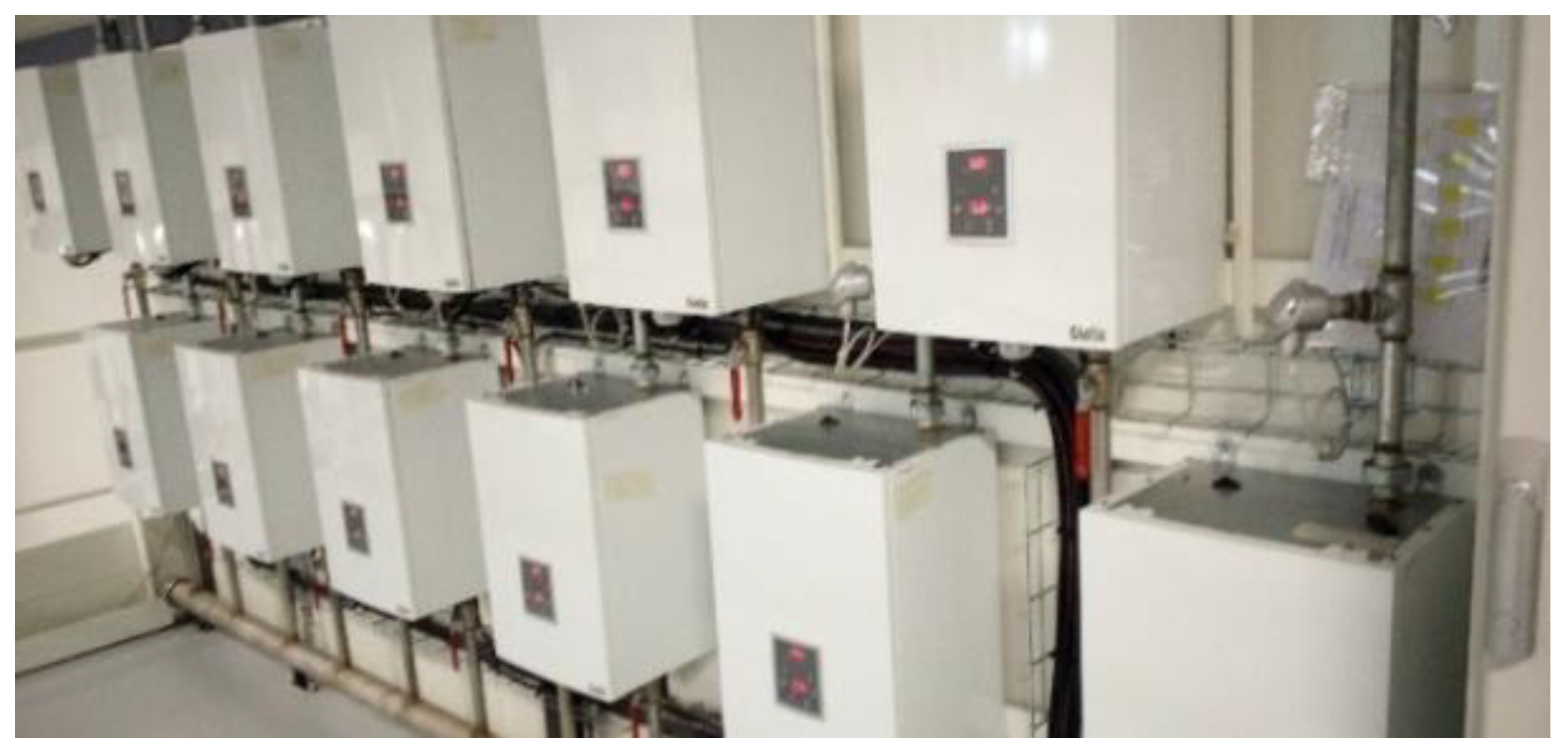
The existence of two thermal loops is clearly justified by the necessity to have a great reactivity at the surface of the envelope. The water in the tank (4) is always set to a much lower temperature than the 36 ones to reach on the envelope (by subtracting two degrees). Because of that, the electrical boilers (Figure 8) are almost continuously switched on to heat the water entering the TAPs. Each one can provide up to 6 kW of power, enabling a great reactivity of the temperature variation. Indeed, some experimentation in the laboratory showed that the target temperature on the surface of the envelope is reached with more accuracy when warming the water than when cooling it. To decrease the temperature of the surface, its associated electrical boiler is switched off, enabling cold water to enter the TAP.
The target temperature for each inner surface of the envelope is calculated and used as a set point every five minutes. So between each time step, the TAPs have five minutes to reach the set point on their respective surface. The next paragraph describes the method used to calculate the set point temperature.
2.3.2. Calculation of the Inner Surface Temperature
There exist quite numerous methods to estimate the thermal behaviour of a wall [18]. However, most of them either don’t consider indoor thermal perturbations or are not accurate enough when estimating the temperature distribution within the wall. As an example, the first order R-C lump method consists of converting a multi-slab wall into an equivalent one-layer wall, disabling the impact of thermal mass position on time lag [19].
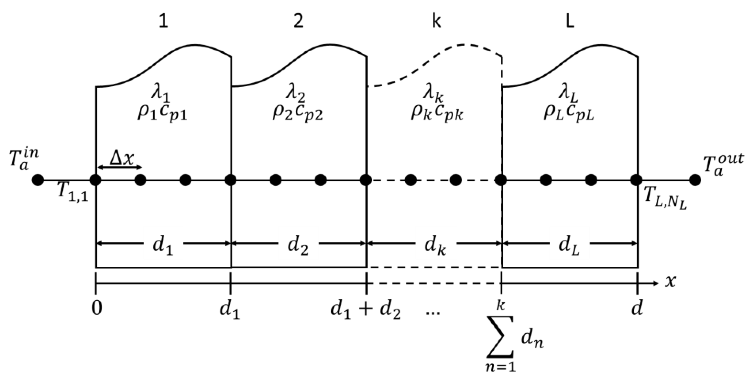
A simple and accurate method to estimate the inner surface temperature of a wall is to analyse its thermal balance and solve the conduction heat equation within the wall in a fundamental way. Under transient conditions, the temperature (T) is a function of the position along with the envelope thickness (x), and the time (t). For a one-dimensional system, the conduction heat transfer is expressed as:
The accuracy when solving Equation (2) depends on the numerical method employed to convert it into an algebraic equation. Pal et al. [20] obtained good results by using the finite difference method for heat transfer modelling on glazing under exposure to solar radiation. Thus, in this study, we combined the well-known explicit finite difference method with Newton’s law at wall boundaries [21].
The explicit finite difference method consists of approximating the derivative terms in Equation (2) by a linear approximation: the first derivative of the temperature with respect to the time and the second derivative of the temperature with respect to the space, at each thermal node along the thickness distribution [22]. Then, we adapted the new algebraic equation for nodes within the layer and for nodes at boundaries between layers. Finally, a thermal balance was made on the inner and outer surfaces of the envelope.
That gives a total of four expressions which represent respectively the temperature at the inner surface (Equation (3)), the temperature of nodes within a layer (Equation (4)), the temperature of nodes at layers’ boundaries (Equation (5)) and finally the temperature at the outer surface (Equation (6)).
where i and j represent time and space indices respectively. The space discretization within the envelope is shown in Figure 9. The temperature at each node is denoted by the symbol where k is the layer index (from inside to outside). The number of nodes varies along the layers since each one has a specific thickness. Thus, a k-layer is given a unique number of nodes, which is noted as . To better read the equations, at each layer, the node counting goes from j = 1 to j = .
The mesh size Δx was set equal to one millimetre to make sure that all boundaries between layers are occupied by a node and to ensure the calculation convergence. Indeed, we assumed that the thickness of a layer is always an integer, given in millimetres. Fixing the mesh size leads to imposing a specific range of time steps for the calculation in order to respect stability criteria for the explicit finite difference method, which is given by:
where α is the thermal diffusivity of the layer. Given that the range of thermal diffusivity is usually between and , the shortest time step for the calculation would be in the range of 0.05 s, which leads to an average of 6000 loops to calculate the target temperature to reach during the five next minutes. This is more than sufficient and not difficult to execute with a standard computer (this calculation is made for the 36 surfaces, which means a total of 216,000 loops are executed).
The radiative and convective heat flux at the surface were combined, using a unique heat transfer coefficient, named hin for the inner surface and hout for the outer surface. In the literature, a large number of expressions can be found for their calculation. It usually depends on the exposition of the wall to other radiative surfaces and air velocity. Wallentén [23] established a non-exhaustive list of different correlations between the heat transfer coefficient and the difference between air temperature and the surface temperature. Usually, it is more appropriate to set the internal heat transfer coefficient as constant since air motion can be considered steady (vair << 1 m/s). It was therefore set at 8 W/m2 K for the inner surfaces: ground, ceiling, and walls. The external heat transfer coefficient is more variable since air motion under outdoor conditions is not steady. For a greater interpretation of air motion, laminar and turbulent flow equations could be taken into account, as shown by Churchill and Chu [24]. However, as a first assumption, we considered the wind behaviour to be close to internal conditions (very low velocity). Thus, the external heat transfer coefficient was set at 25 W/m2 K. Note that these values are also used in the European standard EN 673.
2.4. Measurement Setup
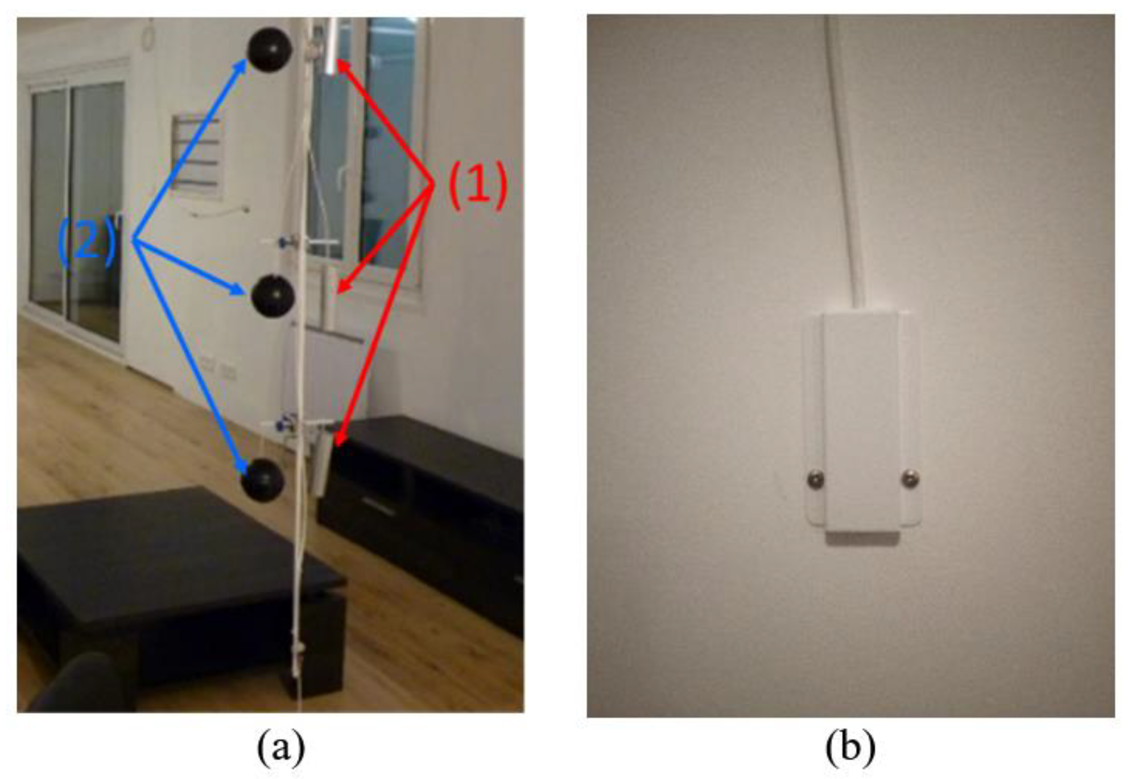
Each temperature-controlled surface is equipped with a sensor placed in its centre. The number of sensors on the envelope is thus equal to 36. In order to increase the measurement precision, the sensors are 4-wire resistance temperature detectors, called PT100 whose technology is well explained by Liu et al. [25]. Their precision was established at 0.04 °C for measurements between 0 °C and 25 °C. All the surface temperature sensors are covered by a small steel white box which isolates them from surrounding radiation and air motion (the right sided picture in Figure 10). That enables the sensor to measure only the surface temperature contribution. In each thermal zone, a measurement mast is placed at the centre (left sided picture in Figure 10). The latter is composed of three pairs of an air temperature sensor placed in a bright aluminium cylinder that works as a radiation shield (1), and a black globe to measure global radiation in the zone (2). The test chamber is composed of ten thermal zones. A preliminary study was performed to establish the critical points to be instrumented in order to record a maximum of efficient data both on the behaviour of the whole housing (and to ensure the proper functioning of the system for reproducing the thermal response of the walls), on the occupant comfort and on the energy consumption of the different thermal zones. In total, 60 sensors are used to measure temperatures. The internal walls and doors were equipped with thermal sensors as well (PT100), totalizing 114 sensors.
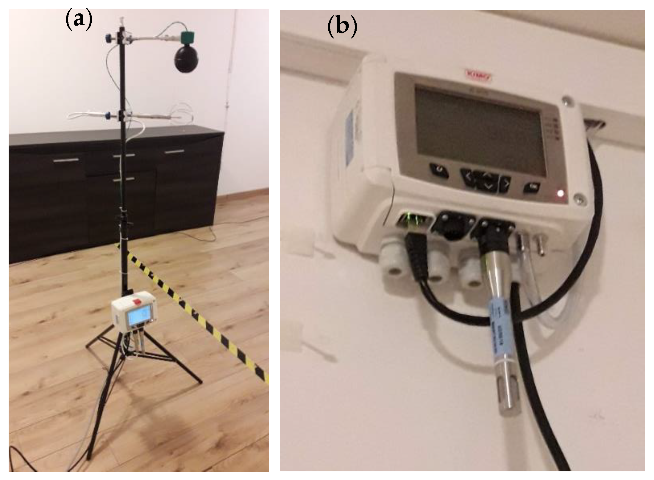
Furthermore, three psychrometric data loggers were placed within the test chamber to evaluate internal psychrometric conditions, as shown in Figure 11. Two mobile masts were also placed in the accommodation. They are equipped with a black globe, an air velocity sensor, and a relative humidity sensor in order to quantify thermal comfort at any place in the test chamber.
In a nutshell, nearly 300 sensors were installed in the test chamber in order to record the regulation parameters of the envelope, the thermal comfort of the occupants, the indoor air quality, and the energy consumption.
2.5. Dynamical Control of the Experimental Facility
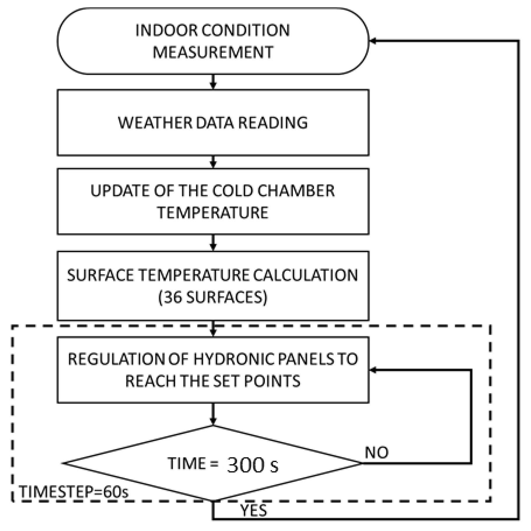
The cold chamber, the TAPs, and the measurement setup are put together in order to reproduce the dynamical thermal behaviour of the building. An experiment campaign works as follows. Before starting experimentation in the test chamber, a weather file and the envelope composition are selected. The thermal properties of the selected materials are then injected into Equations (3)–(6). At initial conditions, we would like to start with an air temperature of say, 20 °C in the test chamber. Therefore, the temperature of the envelope is calculated using a steady state equation in which data from the first line of the weather file and a theoretical indoor air temperature equal to 20 °C are used. All TAPs are then switched on to reach the set point on the envelope. Since the temperature of the envelope is changing, so is the air temperature (either it goes up if the envelope was colder than the set point or it goes down in the opposite situation). Once the indoor air temperature has reached 20 °C, initial conditions are fulfilled, and the experimentation can begin. Then, at each time step, the experimental facility is updated as follows:
- The indoor air temperature, as well as each surface temperature of the envelope, are measured
- The next line of the weather file is read (air temperature and solar radiation)
- The air temperature of the cold chamber is set equal to the one read in the weather file
- Equations (3)–(6) are used to obtain the temperature to reach on the envelope during the next five minutes (for the 36 surfaces)
- TAPs are controlled to reach the set points calculated in step 4
All steps are shown through an organization chart in Figure 12.
The combination of the TAPs and the cold chamber should lead to a good reproduction of the thermal response of the building. The particularity here is that at each time step, the envelope is adapted to the heating system reaction through the air temperature measurement. For example, if heaters stop emitting heat, air temperature stops increasing or even decreases. That behaviour is read by the air temperature sensors and injected into the equations for the new envelope temperature calculation. The latter is thus adapted (according to the materials that were selected at the beginning) to react to that change in thermal evolution. In other words, it is possible in the test chamber to observe the behaviour of heating systems in a wooden house as well as a stone or concrete house. This solution gives “life” to the envelope since it adapts to internal conditions, according to the thermal inertia which has been imposed.
3. Results and Discussion
3.1. Accuracy of the Envelope Temperature Regulation
Preliminary tests were made to calibrate the PI loop coefficients for the TAPs regulation. The objective was to make sure that the target set point was respected and that the temperature change rate is high enough. To do so, the air temperature inside the test chamber was controlled and set to 18 °C during all the experimentations so that it did not affect the calibration of the TAPs. The latter was then made according to Ziegler Nichols’ method [26].
Figure 13 shows the temperature evolution of a wall after calibrating the PI coefficients (upper graph). All surfaces were set to the same target set point. As seen in the figure, a 1 °C temperature step was applied, then a 0.5 °C step, and finally two progressive increases/decreases were applied, with a 0.1 °C step for the first one and a 0.2 °C step for the second one. Both were applied with a 10-min-long time step for each set point. For the first three types of step change, the demanded reactivity was respected. However, increasing the temperature by 0.2 °C in less than ten minutes seems to be difficult and not steady. The overall standard deviation between the surface temperature and the target set point (lower graph) was 0.1 °C, which included the temperature difference right after the set point modification. When we focus only on steady-state conditions, the standard deviation drops to 0.05 °C, which is at the edge of the temperature sensor’s accuracy.
However, it was not realistic to keep the air temperature at a constant level while increasing the envelope temperature. The larger the temperature difference between both, the more difficult it is to control the envelope temperature with precision, and that explained the error increase at the last type of step change. So, it means that in real conditions, where the air temperature stays close to the envelope temperature, the error after a step change of temperature would be less than 0.1 °C. This result is very satisfying given that it is not relevant to measure temperatures with better precision than 0.1 °C. In addition, looking at the rate of change of temperature on the envelope, the thermal inertia limits that could be set on the envelope varies from very low insulation (just a layer of plasterboard) to very high insulation (beyond the energy label recommendations).
3.2. Analysis of the Thermal Inertia Controlling in the Test Chamber
The PI control loops were calibrated and thus, a great accuracy was observed. The thermal regulation of the envelope is therefore considered satisfying. It is now possible to analyse the thermal inertia controlling in the test chamber. That analysis and the following ones were made by using the simulation model in TRNSYS 17.
A wide variety of building energy simulation programs have been developed, enhanced, and are in use throughout the building energy community [27]. Our industrial needs led us to select TRNSYS 17 for its user-friendly interface and the large number of features that are available. Apart from being powerful and robust, TRNSYS 17 is widely used for thermal calculations in buildings, both for the envelope thermal behavior and for the energy consumption. Therefore, a simulation model of the test chamber was developed in TRNSYS 17, in which thermal and aeraulic transfer were combined by using the extension called TRNFLOW. This extension considers air flows between air nodes and thus, enables to better estimate heat transfer by aeraulic exchanges in the building. The simulation model of the test chamber was developed following its architecture which is composed of twelves air nodes. Each air node is connected to its adjacent ones by air flow links. These links depict either wide openings (e.g., doors) or ducts (e.g., ventilation system). The wide openings are defined by Bernoulli’s equations, in which the discharge coefficient is a function of the openings’ height. For doors, which the dimensions are rather similar worldwide, the Pelletret approach showed great satisfaction [28]. The air flow in ducts is characterized by the friction losses and the dynamic losses coefficient which depend on the ventilation network configuration (length, section, and flexions). In TRNFLOW, the ventilation network is not defined in terms of dimensions but by the dynamic losses coefficient, which can be determined by experimentation. Its value is calculated later on in this subsection. The inner and outer surface temperatures are calculated by the conduction heat transfer function, developed by Mitalas [29], which depends on each layer’s thermal properties. The conduction transfer function is a time series allowing to calculate the inside and outside heat fluxes from current and previous values of the surface temperatures and the heat fluxes themselves. This method leads to short-time calculations.
As a first step, the analysis was done without any heating system. The objective was to verify that the set of equations used to calculate the inner surface temperatures of the envelope works fine. Only the ventilation system was on, set as a single flow.
Two types of envelope composition were selected. The first one was a light thermal mass house, which will be referred to as a “light mass envelope” and the second one was a heavy thermal mass house, referred to as a “heavy mass envelope”. Their composition, shown in Table 1, was adapted from case 900 of the BesTest series [30]. The floor and the ceiling were the same in both envelopes. The only difference is in the walls, where the insulation layer is placed inside the building for the light mass envelope and outside the building for the heavy mass envelope. The composition of the ceiling is the same in both setups with a very low thermal mass. Here, the goal was to observe the heat transfer in two different thermal mass envelopes but with the same insulation rate.
Using the methodology of Chahwane [31], the time constant for both cases was calculated. The light mass envelope had a 20-h-long time constant, while the heavy mass envelope had a 90-h-long time constant. There was a 70-h-long gap between both, which enabled us to make relevant assumptions on the performance of the test chamber for light as well as heavy envelope compositions.
For this kind of test, no weather file was used. Instead, only the outdoor dry-bulb temperature was considered, which was defined as:
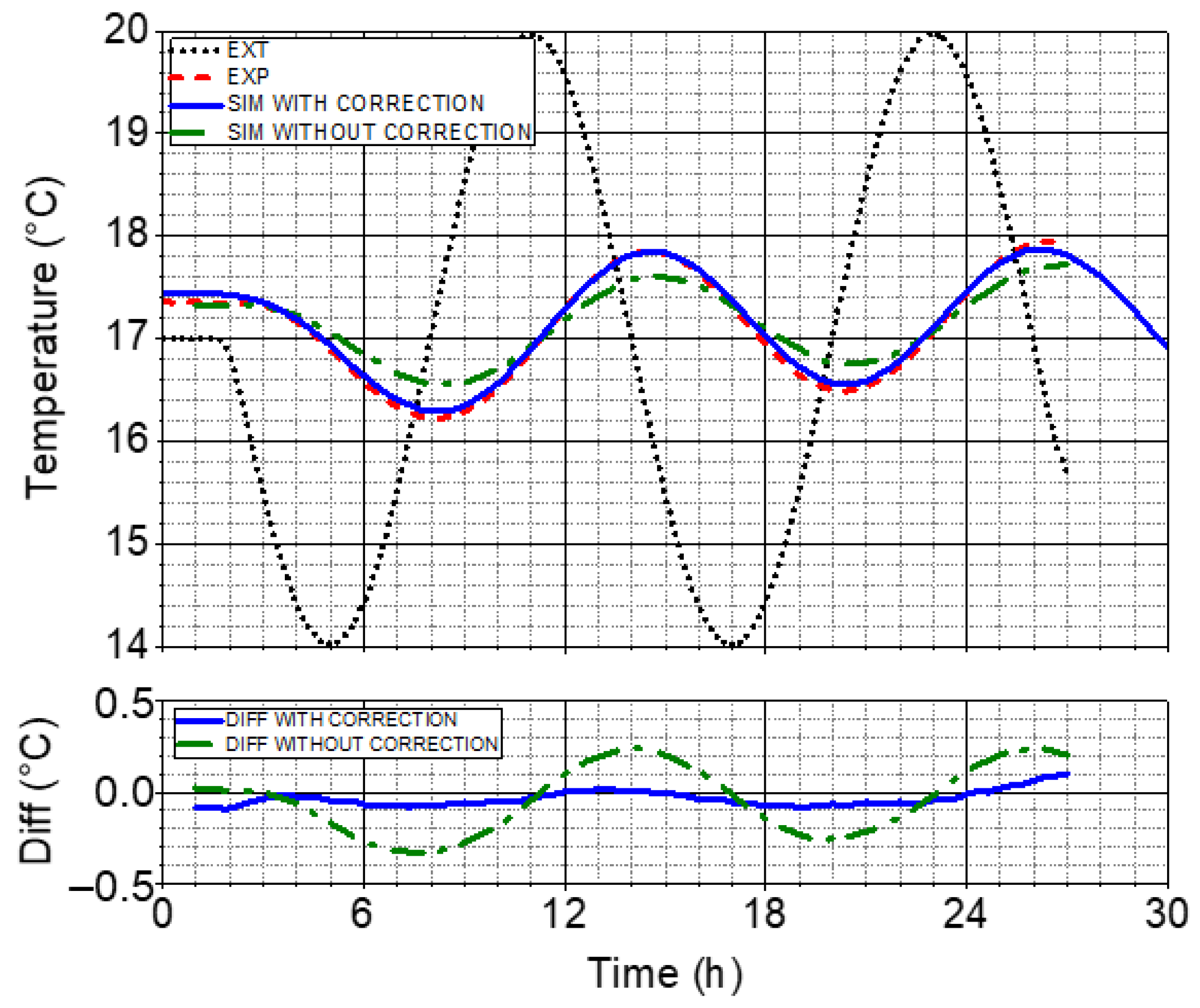
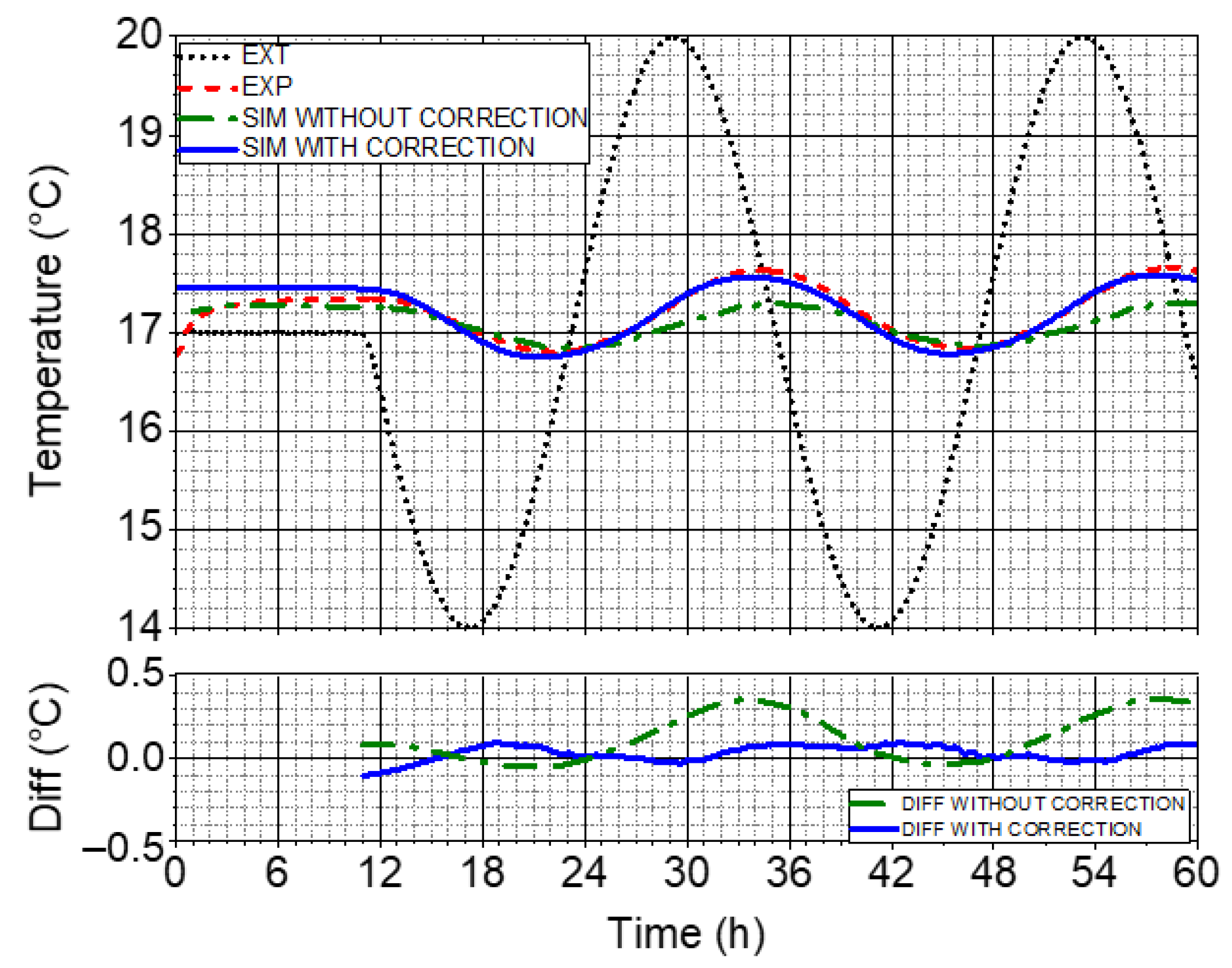
where B, the oscillation period, was set to 12 h during the light mass experimentation, and 24 h during the heavy mass experimentation. The other weather parameters were set equal to neutral (the sky and ground temperatures were set equal to the outdoor dry-bulb temperature). All surfaces of the envelope, including ground surfaces, were assumed to be exposed to the outside conditions to simplify the analysis.
A first analysis of the mean air temperature within the test chamber with the light and heavy mass envelope configuration showed a slight difference with the simulation, as shown in Figure 14 and Figure 15 by looking at the “SIM WITHOUT CORRECTION” curve. The decrement factor seemed higher in the simulation approach than in the experimentation. An investigation of factors that could explain that difference led to two conclusions.
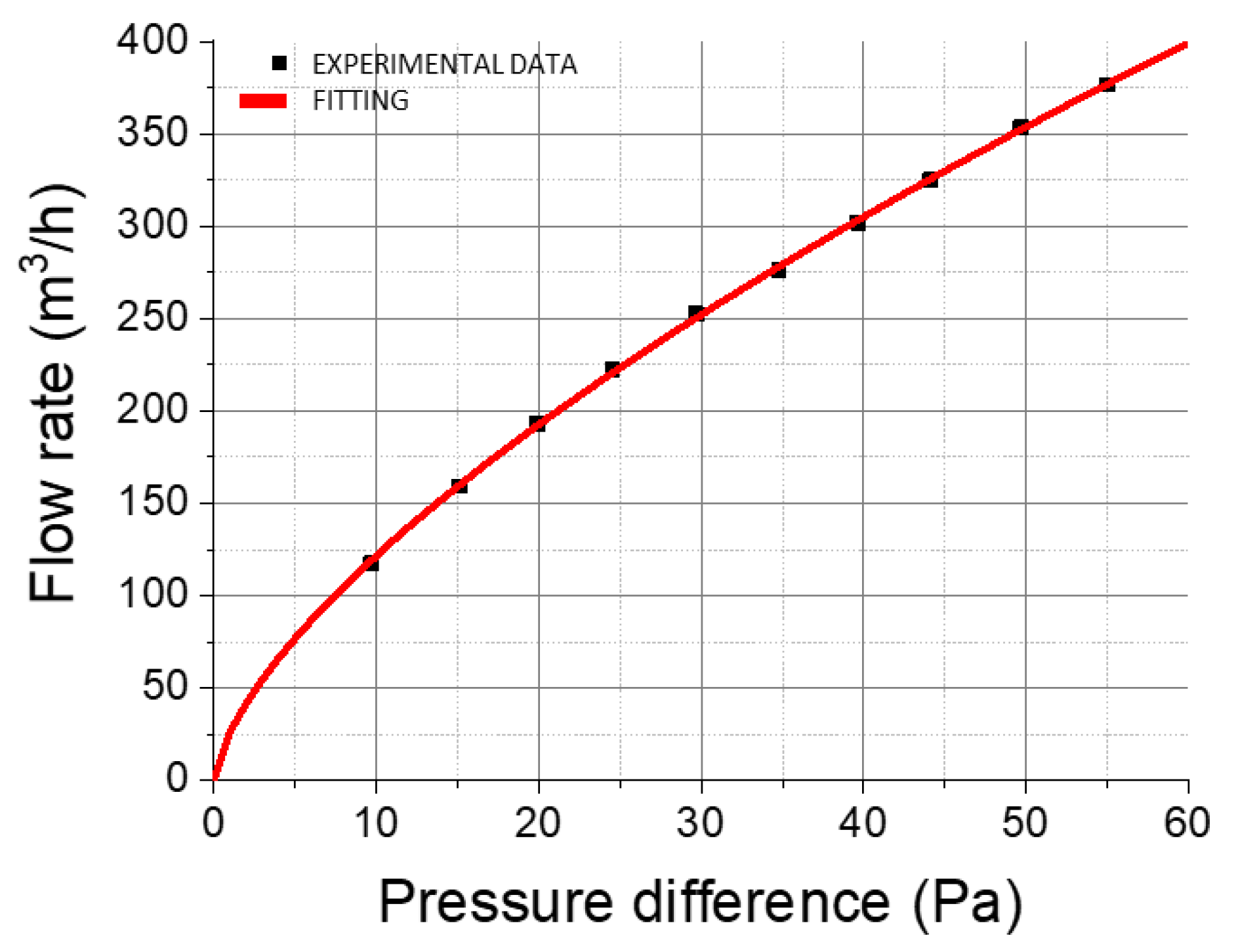
The first one was that there exists an air leakage in the test chamber that wasn’t set in the simulation approach. To investigate this, a blow door test was made in order to quantify this air leakage rate. Figure 16 shows the measured flow rate of the air leakage as a function of the pressure difference between indoor and outdoor (black square dots).
A fitting of the experimental data (red line in Figure 16) shows that it perfectly matches air leakage’s law [32]. The expression between pressure difference and air flow is given by:
The second conclusion was on the ventilation network in the simulation model. Air flows within ventilation ducts are characterized by the dynamic losses coefficient ξ [29], which was set initially at 1 in the absence of information. Its expression is given by:
where is the pressure difference at the opening of the duct, S is the section of the duct, is the density of air and is the air flow rate in the duct. Measurements in the test chamber were made in order to quantify this dynamic loss coefficient. Finally, a coefficient equal to 20 was set in the simulation model.
The expression giving the infiltration rate (Equation (9)) as well as the new dynamic loss coefficient (Equation (10)) were integrated with the simulation model. As a result, simulation and experimentation matched with great accuracy, as shown by the “SIM WITH CORRECTION” curve in Figure 14 and Figure 15. In both cases, the error between simulation and experimentation dropped below 0.1 °C and the standard deviation dropped to 0.04 °C, which was equal to the accuracy of the sensors.
The results from the two different mass envelopes confirm that the equation system, used to calculate the temperature of each surface of the envelope, is well established and provides a good adaptation of the envelope regarding the thermal inertia imposed prior to beginning the experimentation. Thus, the combination of the cold chamber and the TAPs led to a reliable reproduction of the thermal inertia within the test chamber. However, those results were obtained without heating systems. Another analysis must be done by adding heaters to assess the behaviour of the TAP when dynamic heat fluxes occur.
3.3. Analysis of the Thermal Response Reproduction in the Presence of a Heating System
When a heating system is installed in the test chamber, the global air temperature evolution is expressed by:
where φheat is the heating power, φwind is the heat transfer by ventilation, φleak is the heat transfer by air leakage, is the envelope temperature, hin is the heat transfer coefficient on the envelope, and S is the total area of the envelope. It means that when an internal power is put into the accommodation, the envelope behaviour adapts itself to the generated perturbations. The objective of this analysis is to confirm that the TAPs in the test chamber can take heating into account and adapt the envelope temperature according to the composition that is imposed.
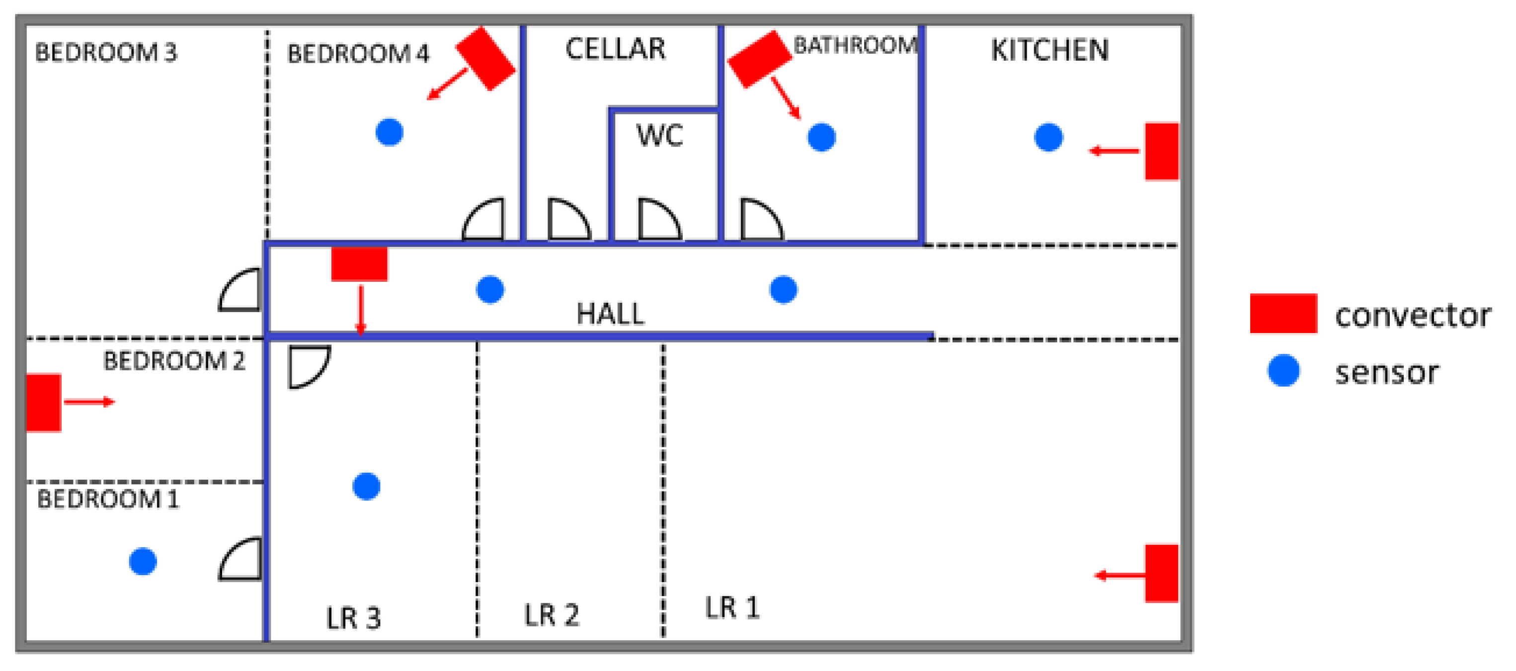
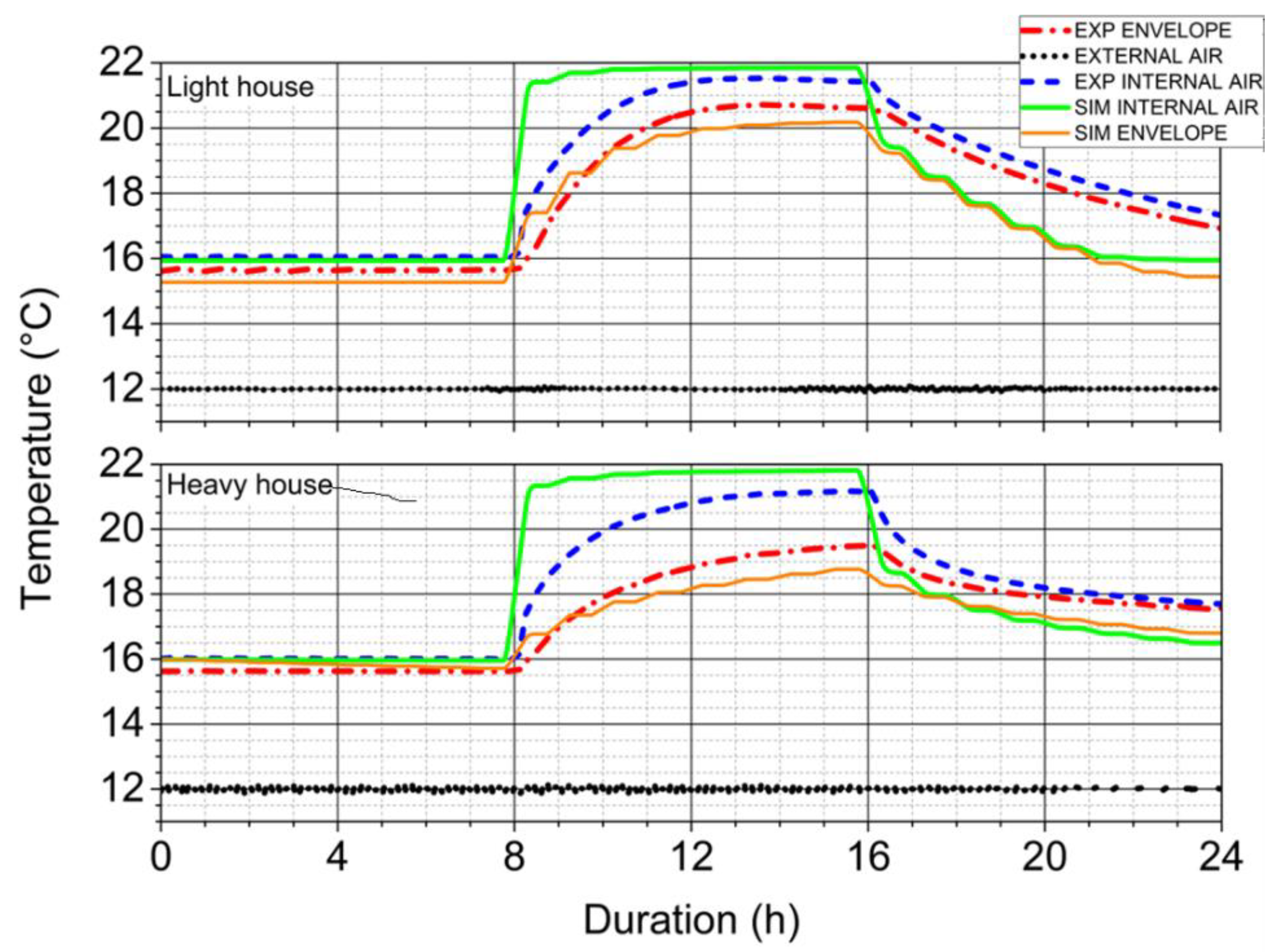
To do that, six convectors were placed in the accommodation. Each one can provide 1000 W of heating power. Their position was set so that heat diffusion is optimized, as shown in Figure 17. The heating temperature set point was set at 22 °C (COMFORT mode), while the economic temperature set point was set at 16 °C (ECO mode). The experimentation duration was 24 h divided into three parts: 8 h of ECO mode, 8 h of COMFORT mode, and 8 h of ECO mode. Finally, the outside air temperature was set at 12 °C constantly, to create permanent heat loss from the envelope.
Figure 18 shows the temperature evolution (average of all rooms to make it easier to read) measured in the test chamber and also calculated in the simulation model for both types of thermal mass envelope. The graphs clearly show a quite significant difference between the measurements and the calculations. In the simulation, the average air temperature reached the set point in less than one hour in both types of thermal mass while in the experimentation, it took around four hours in the light thermal mass envelope and more than eight hours in the heavy thermal mass envelope. In the latter case, the set point was not even reached before the end of the COMFORT mode.
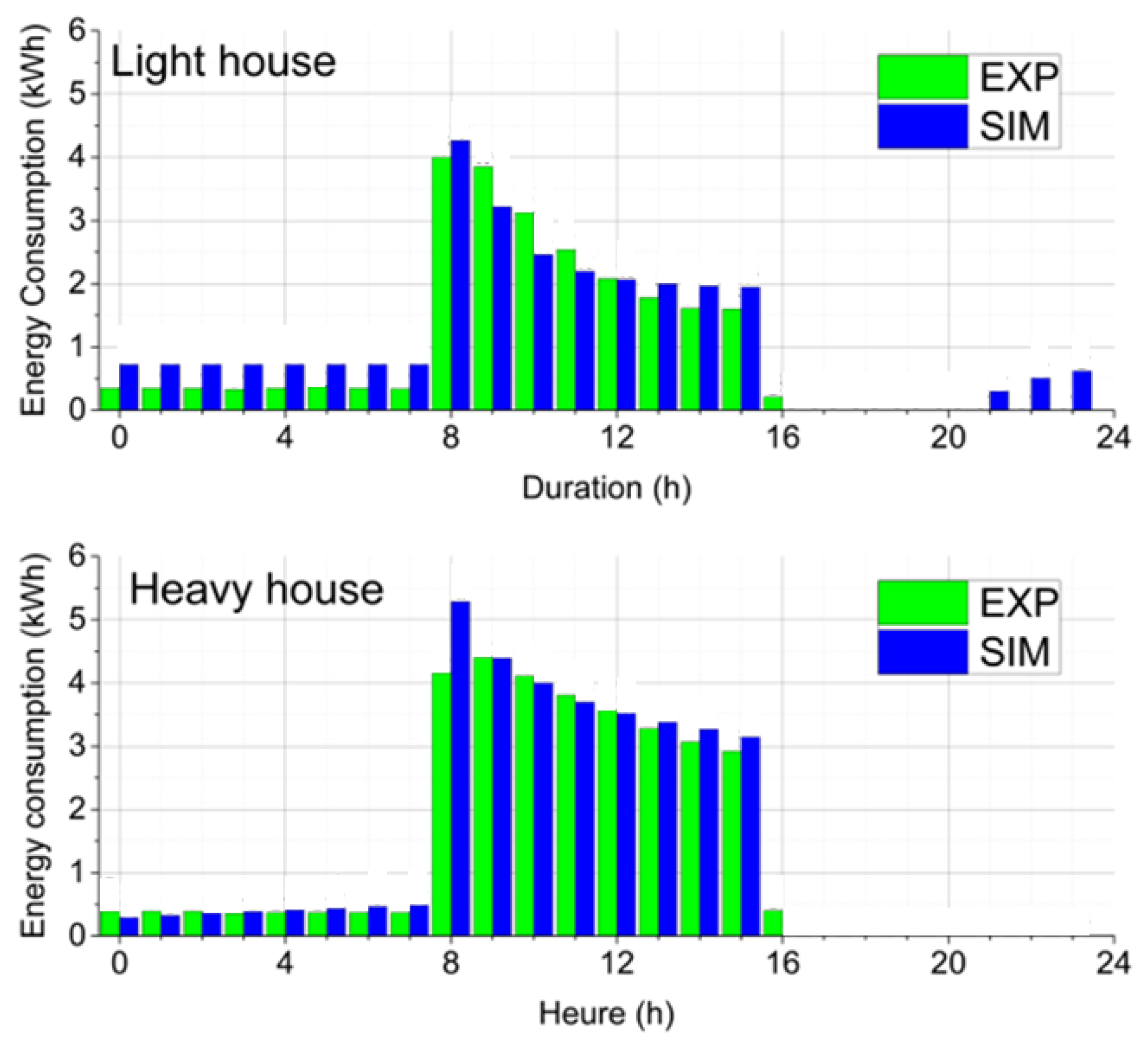
An interesting point is that the average temperature of the envelope is quite similar in simulation and experimentation during the COMFORT period (dashed point curve and solid thin curve). The same particularity was observed when looking at the energy consumption (Figure 19). Two observations can be formulated from these particularities. The first one stipulates that in the simulation, the power of heating is immediately transferred to all the volume of the building. In reality, and as shown in the experimentation, heaters need some time to increase in temperature, then some time is needed for heat to be diffused in all the volumes. This is why the average air temperature behaves more like a lumped capacitance model in the experimentation than in the simulation.
The second observation stipulates that the internal heat transfer coefficient (hin) on the envelope was not equal in the simulation and the experimentation during the test. In both approaches, hin was set equal to 8 W/m2 K, however, in reality (which is in the experimental approach), air motion was dependent on the heaters which created turbulent air flows. According to the measured data and calculations, hin started at around 3 W/m2 K before switching the heaters on and ended at almost 20 W/m2 K after. The more hin increases, the higher the heat transfer between the air volume and the envelope. But since the envelope was colder than the air, more thermal exchanges meant slower air temperature increase. That is why the increase in air temperature was slower in the experimentation. The heat transfer coefficient hin must be adapted at each time step. For this purpose, the implementation of flow mechanics laws could be established but this solution would need to measure air velocity on each surface. A good approximation would be to use Equation (11). Indeed, at each time step, every term in the equation is known by measurement except hin. It would be possible then to calculate it, using Equation (10) and to inject it into Equations (2)–(6). With this method, heat transfer on the envelope would be more realistic. That method is currently in development and will be tested later on, as the first results provide reliable enough conclusions on the heating system behaviour against the thermal mass of the envelope.
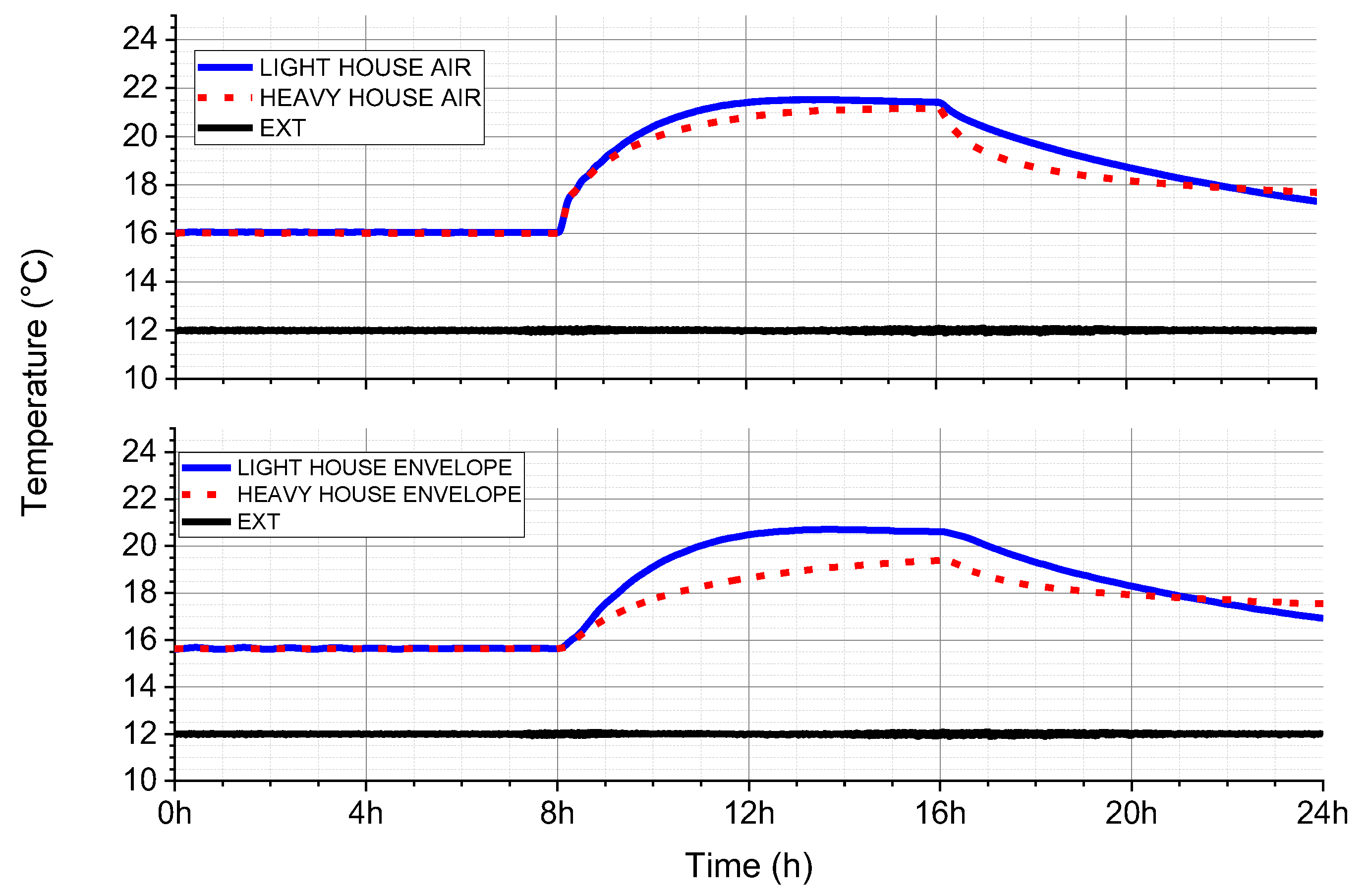
One important statement here is that, despite those two observations, the thermal behaviour in the experimentation was still more realistic than in the simulation, where air temperature evolution was too “ideal”. Applying a constant value on hin did not prevent the wall’s temperature to vary according to the thermal mass of the envelope. A significant difference between the light mass envelope and the heavy one can be observed in Figure 20, which derives from Figure 19, which was rearranged in order to show the air temperature and the envelope temperature evolution in the experimentation approach only.
As expected, when the heaters were turned on, the envelope temperature evolution was more reactive with the light mass envelope. The TAPs clearly controlled the thermal evolution rate of the envelope. The latter hardly reached 19 °C in the heavy mass envelope while it passed above 21 °C in the light mass envelope. At 16 h, when the heaters went from COMFORT mode to ECO mode, the air temperature started decreasing. In the heavy mass envelope, the decrease was faster than in the light mass envelope, unlike the expectations. Actually, at 16 h, the envelope temperature in the heavy mass envelope was lower than in the light mass envelope, leading, through heat transfer with the envelope, to a faster decrease of the air temperature. Actually, this first cycle of COMFORT/ECO mode could be compared to a typical first day of heating in a holiday house, where the envelope is still in the process of storing energy. After several days of heating in the COMFORT/ECO mode, the air temperature in the heavy mass envelope would obviously decrease slower than in the light mass envelope in ECO mode.
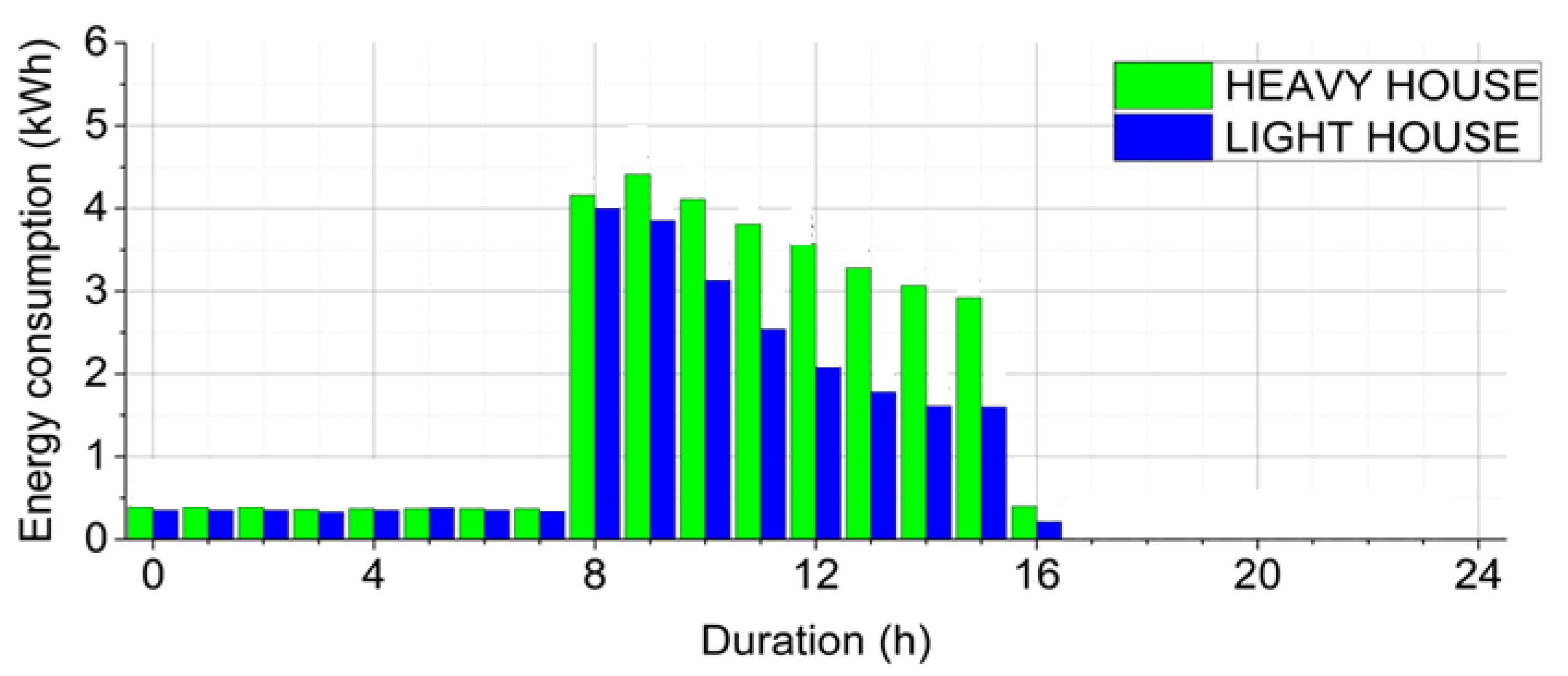
The difference in reactivity in both envelope compositions was confirmed by looking at the energy consumption, shown in Figure 21. The energy demand for the heavy mass envelope was higher than in the light mass envelope, due to the initial conditions. Indeed, before entering the COMFORT mode, the internal conditions were the same for both envelopes (giving the same energy consumption since both envelopes have the same insulation rate). Due to the thermal mass of the heavy envelope, the first heating cycle required a lot of energy. At the end of the day (24 h), the mean air temperature was higher in the heavy mass envelope, which means that its thermal inertia had stored more energy. Thus, the next cycle would have demanded less energy, and so on, until the energy demand would get lower than in the light mass envelope. That conclusion proves that the experimental platform is clearly able to reproduce the impact of thermal inertia.
Doors and windows are not discussed in this study, because the objective is to demonstrate the ability to reproduce any type of envelope inertia and weather conditions with the TAPs and the cold chamber. In perspective, the doors and windows can simply be replaced to test other products.
3.4. Advantages and Limits of the Experimental Facility
By looking at the results of the thermal response of the test chamber with different thermal masses, different outside conditions, and heaters, it can be admitted that the combination of the cold chamber and the TAPs cover most of the parameters that control heat transfer on the building. Thanks to the control of the outside air temperature and the envelope thermal behaviour, the test chamber can be placed under any type of weather, from north European to the Mediterranean climate, and reproduce the thermal behaviour of any type of house. Unlike the twin houses from the Fraunhofer Institute [13], which cannot be modified and are exposed to actual weather, or the INCAS houses from the CEA Institute [14], which are exposed to the actual weather and provide only four types of construction. In the experimental chamber, the ventilation system can be changed in order to assess different technologies of the ventilation system. One element that was not mentioned yet is the ability to modify the orientation of the test chamber. Indeed, it is very simple to change it by modifying the wind characteristics and the solar heat gain in Equations (3)–(6) for each wall. It is also possible to set the test chamber as a flat in a building by adapting the equations for the ground and the ceiling so that the boundary conditions represent the thermal behaviour of adjacent accommodations (for example, by setting the solar heat gain and the wind velocity at zero and setting the outside air temperature to a typical accommodation thermal evolution). Regarding all those qualities, the experimental facility described in this paper provides a wide range of degrees of liberty to perform thermal experimentations, and thus, it represents a more efficient tool for energy performances and thermal comfort assessment. One possible application would be to perform certification tests on thermal systems in the future where test conditions will have to be closer to reality. Another possible application would be to assess the performances of the thermal systems against the global warming evolution, for example, exposing the thermal systems to progressively warmer outside conditions.
However, two key elements were not reproduced yet in the experimental facility: direct solar heat gain through the glazing and the occupants’ activity. The solar heat gains through could be reproduced by using specific lamps, but it seems very costly and not very efficient [33]. Instead, the direct solar radiation impact through glazing will be directly reproduced by heating the sunspots in the test chamber. Future development will consist of the development of a numerical tool to calculate the position of the sunspots and their surface temperature. Then, by using a mesh of electric films on the ground, the sunspots will be heated to reach their set point. Thanks to the mesh it will be possible to move the heated sunspots as a function of time and sun position.
The effects of occupants’ activity are not discussed in this article as it is the next step of development. It will be reproduced by controlling all of the electric devices and openings in the test chamber using automation systems.
4. Conclusions
In an attempt to better analyse the interactions between the heating systems and their environment, a new generation of the experimental facility was developed. The novelty here lies in the possibility of controlling the thermal performance of the building, the room’s layout, and the weather conditions without modifying its external structure.
A description of the two main technical solutions that were adopted to develop the experimental facility was made. The first one is a cold chamber, placed all around the accommodation, and in which the air temperature is dynamically controlled from −10 °C to +20 °C. The second solution is the thermally active panels that were placed on the envelope to accurately control its inner surface temperature, calculated with the finite difference method. The aim was to adapt the temperature of the envelope according to indoor conditions and the thermal inertia of the building to study.
A first measurement campaign was made in order to characterize the performances of the thermally active panels and the cold chamber. Then a second measurement campaign aimed to compare the behaviour of the experimental facility for two opposite thermal inertia of the envelope (light and heavy thermal inertia).
The first results showed that using thermally active panels to dynamically control the temperature of the envelope is an efficient tool that provides a high accuracy level. The standard deviation between the target set point and the measurement was at the edge of the measurement accuracy (0.05 °C). The results also show that the cold chamber is highly reactive and gives good control of the outside air temperature evolution. It is possible to reproduce any French climate, up to North European climates, and to study any type of envelope composition from very low insulated (just one layer of plasterboard) to the high insulated envelope (beyond recommended regulatory value).
The second results show that the equation system obtained from the finite difference method enabled the adaptation of the thermal behaviour of the envelope with good precision. Thanks to the simulation model, it was possible to confirm the good reproduction of the thermal response in the experimental platform when the heating systems were turned off.
Finally, a heating system was installed in the accommodation. The observation of the air temperature evolution for two different thermal inertia in the test chamber showed that the heating devices did work as if they were in two different houses, leading to different energy consumption. However, some optimization must be done on the heat transfer coefficient hin. As a first step, it was fixed as a constant, but it must be calculated at each time step and integrated into the system of equations to better adapt the temperature of the envelope to the real internal conditions.
This study showed that it is already possible to study the heating system behaviour in different thermal inertia using this experimental facility. The next step would be to integrate the activity of the occupant and the solar heat gains through the glazing. It then would be possible to study the heating systems as a function of the complete environment that is met usually in a real case. This experimental facility could become a new investigation tool for R&D, a certification tool in more realistic outside conditions, and is a real proof of concept for assessing the thermal systems against global warming (progressively warmer thermal conditions).
Author Contributions
Conceptualization, O.D. and T.L.; methodology, G.P.; validation, W.F., O.D. and A.D.T.L.; formal analysis, G.P.; investigation, W.F.; resources, T.L.; writing—original draft preparation, W.F.; writing—review and editing, O.D. and G.P.; visualization, A.D.T.L.; supervision, O.D.; project administration, T.L.; funding acquisition, O.D. and T.L. All authors have read and agreed to the published version of the manuscript.
Funding
This research was funded by Hauts-de-France Council, through IndustriLab grant.
Institutional Review Board Statement
Not applicable.
Informed Consent Statement
Not applicable.
Data Availability Statement
Not applicable.
Acknowledgments
The authors would like to thank the Hauts-de-France Region for funding this work under the IndustriLab grant, and Groupe Muller for supporting and funding this work.
Conflicts of Interest
The authors declare no conflict of interest. The funders had no role in the design of the study; in the collection, analyses, or interpretation of data; in the writing of the manuscript, or in the decision to publish the results.
Nomenclature
| α | Thermal diffusivity | |
| Δt | Time step | |
| Δx | Mesh space step | |
| λ | Thermal conductivity | |
| φ | Heat flux | |
| ρ | Density | |
| Specific heat | ||
| h | Heat transfer coefficient | |
| Fo | Fourier number | |
| T | Temperature | |
| [ | Air flow |
References
- Guo, Y.; Wang, J.; Chen, H.; Li, G. Machine learning-based thermal response time ahead energy demand prediction for building heating systems. Appl. Energy 2018, 221, 16–27. [Google Scholar] [CrossRef]
- Bianchini, G.; Casini, M.; Vicino, A.; Zarrilli, D. Demand-response in building heating systems: A model predictive control approach. Appl. Energy 2016, 168, 159–170. [Google Scholar] [CrossRef]
- Chiffres clés de l’énergie Commissariat Général au Développement Durable. 2018. Available online: https://www.statistiques.developpement-durable.gouv.fr/sites/default/files/2018–10/datalab-43-chiffres-cles-de-l-energie-edition-_2018-septembre2018.pdf (accessed on 13 November 2021).
- Ürge-Vorsatza, D.; Cabeza, L.F.; Serrano, S.; Barreneche, C.; Petrichenko, K. Heating and cooling energy trends and drivers in buildings. Renew. Sustain. Energy Rev. 2015, 41, 85–98. [Google Scholar] [CrossRef] [Green Version]
- Aditya, L.; Mahliaa, T.M.I.; Rismanchi, B.; Ng, H.M.; Hasane, M.H.; Metselaar, H.S.C.; Muraza, O.; Aditiya, H.B. A review on insulation materials for energy conservation in buildings. Renew. Sustain. Energy Rev. 2017, 73, 1352–1365. [Google Scholar] [CrossRef]
- Jelle, B.P. Traditional, state-of-the-art and future thermal building insulation materials and solutions–Properties, requirements and possibilities. Energy Build. 2011, 43, 2549–2563. [Google Scholar] [CrossRef] [Green Version]
- Gönülol, O.; Tokuç, A. Net zero energy residential building architecture in the future. In Exergetic, Energetic and Environmental Dimensions; Dincer, I., Colpan, C.O., Kizilkan, O., Eds.; Academic Press: Cambridge, MA, USA, 2018; pp. 39–53. [Google Scholar]
- Bond, D.E.M.; Clark, W.W.; Kimber, M. Configuring wall layers for improved insulation performance. Appl. Energy 2013, 112, 235–245. [Google Scholar] [CrossRef]
- Schakib-Ekbatan, K.; Çakıcı, F.Z.; Schweiker, M.; Wagner, A. Does the occupant behavior match the energy concept of the building?—Analysis of a German naturally ventilated office building. Build. Environ. 2015, 84, 142–150. [Google Scholar] [CrossRef]
- Foucquier, A.; Robert, S.; Suard, F.; Stéphan, L.; Jay, A. State of the art in building modelling and energy performances prediction: A review. Renew. Sustain. Energy Rev. 2013, 23, 272–288. [Google Scholar] [CrossRef] [Green Version]
- Luo, N.; Weng, W.G.; Fu, M.; Yang, J.; Han, Z.Y. Experimental study of the effects of human movement on the convective heat transfer coefficient. Exp. Therm. Fluid Sci. 2014, 57, 40–56. [Google Scholar] [CrossRef]
- Tian, W.; Han, X.; Zuo, W.; Sohn, M.D. Building energy simulation coupled with CFD for indoor environment: A critical review and recent applications. Energy Build. 2018, 165, 184–199. [Google Scholar] [CrossRef]
- Fraunhofer, Twin Houses, Energy Efficiency and Indoor Climate. Fraunhofer Institute. Available online: https://www.ibp.fraunhofer.de/en/press-media/research-in-focus/reality-check.html (accessed on 13 November 2021).
- Spitz, C. Analysis of Simulation Tools Reliability and Measurement Uncertainties for Energy Efficiency in Buildings. Ph.D. Thesis, Université de Grenoble, Saint-Martin-d’Hères, France, March 2012. [Google Scholar]
- Sun, C.; Shu, S.; Ding, G.; Zhang, X.; Hu, X. Investigation of time lags and decrement factors for different building outside temperatures. Energy Build. 2013, 61, 1–7. [Google Scholar] [CrossRef]
- Housing Conditions in France. 2022 INSEE Survey. Available online: https://www.insee.fr/fr/statistiques/fichier/2586377/LOGFRA17.pdf (accessed on 22 February 2022).
- Mazzeo, D.; Oliveti, G.; Arcuri, N. Influence of internal and external boundary conditions on the decrement factor and time lag heat flux of building walls in steady periodic regime. Appl. Energy 2016, 164, 509–531. [Google Scholar] [CrossRef]
- Lefebvre, G. Comportement Thermique Dynamique des Parois Planes. Technique de l’Ingénieur 1992. Available online: https://www.techniques-ingenieur.fr/base-documentaire/tiabeb-archives-ressources-energetiques-et-stockage/download/b2040/1/comportement-thermique-dynamique-des-parois-planes.html (accessed on 14 December 2021).
- Fraisse, G.; Viardot, C.; Lafaabrie, O.; Achard, G. Development of a simplified and accurate building model based on electrical analogy. Energy Build. 2002, 34, 1017–1031. [Google Scholar] [CrossRef]
- Pal, S.; Roy, B.; Neogi, S. Heat transfer modelling on windows and glazing under the exposure of solar radiation. Energy Build. 2009, 41, 654–661. [Google Scholar] [CrossRef]
- Incropera, F.P.; DeWitt, D.P.; Bergman, T.L.; Lavine, A.S. Fundamentals of Heat and Mass Transfer; Wiley: New York, NY, USA, 2007. [Google Scholar]
- Lienhard, J.H., IV; Lienhard, J.H., V. A Heat Transfer Textbook, 5th ed.; Phlogiston Press: Cambridge, MA, USA, 2019. [Google Scholar]
- Wallentén, P. Convective heat transfer coefficients in a full-scale room with and without furniture. Build. Environ. 2001, 36, 743–751. [Google Scholar] [CrossRef]
- Churchill, S.W.; Chu, H.H.S. Correlating equations for laminar and turbulent free convection from a vertical plate. Int. J. Heat Mass Transf. 1975, 18, 1323–1329. [Google Scholar] [CrossRef]
- Liu, J.; Li, Y.; Zhao, H. A temperature measurement system based on PT100. In Proceedings of the International Conference on Electrical and Control Engineering, Wuhan, China, 25–27 June 2010. [Google Scholar]
- Copeland, B.R. The Design of PID Controllers Using Ziegler Nichols Tuning. 2008. Available online: http://educypedia.karadimov.info/library/Ziegler_Nichols.pdf (accessed on 25 September 2020).
- Crawley, D.B.; Hand, J.; Kummert, M.; Griffith, B.T. Contrasting the capabilities of building energy performance simulation programs. Build. Environ. 2008, 43, 661–673. [Google Scholar] [CrossRef] [Green Version]
- Pelletret, R.; Liebecq, G.; Allard, F.; Van Der Maas, J. Modelling of large openings. In Proceedings of the 12th Conference on Air Movement and Ventilation Control Within Buildings, Ottawa, ON, Canada, 24–27 September 1991. [Google Scholar]
- Mitalas, G.; Arseneault, J. Fortran IV Program to Calculate z-Transfer Functions for the Calculation of Transient Heat Transfer Through Walls and Roofs, 1972, NRC. Available online: https://nrc-publications.canada.ca/eng/view/fulltext/?id=9a383a07-6830-401d-a3a7-ab15ad077208 (accessed on 7 June 2020).
- Henninger, R.H.; Witte, M.J. EnergyPlus Testing with ANSI/ASHRAE Standard 140-2001 (BESTEST). 2004. Available online: https://simulationresearch.lbl.gov/dirpubs/epl_bestest_ash.pdf (accessed on 18 July 2020).
- Chahwane, L. Valorization of Thermal Mass for the Energy Performances of Buildings. Ph.D. Thesis, Université de Grenoble, Saint-Martin-d’Hères, France, October 2011. [Google Scholar]
- Bilsborrow, R.E.; Fricke, F.R. Model verification of analogue infiltration predictions. Build. Sci. 1975, 10, 217–230. [Google Scholar] [CrossRef]
- Meng, Q.; Wang, Y.; Zhang, L. Irradiance characteristics and optimization design of a large-scale solar simulator. Sol. Energy 2011, 85, 1758–1767. [Google Scholar] [CrossRef]
Figure 1.
Illustration of the interior of the experimental facility.

Figure 2.
Plan of the test chamber (view from above).

Figure 3.
Envelope composition of the test chamber.

Figure 4.
Air temperature evolution in the cold chamber.

Figure 5.
Ventilation network for the two ventilation systems—(a) dual air flow system, (b) single air flow system.
Figure 5.
Ventilation network for the two ventilation systems—(a) dual air flow system, (b) single air flow system.

Figure 6.
Thermal active panels cutting.

Figure 7.
The temperature control loop of the hydronic panels.

Figure 8.
Electrical boilers.

Figure 9.
Discretization of a multi-layer wall.

Figure 10.
Sensors in the experimental facility. (a) a measurement mast. (b) a wall temperature sensor.
Figure 10.
Sensors in the experimental facility. (a) a measurement mast. (b) a wall temperature sensor.

Figure 11.
(a) a mobile measurement mast. (b) a psychrometric data logger.

Figure 12.
Control process of the experimental facility.

Figure 13.
Temperature evolution of a wall for different temperature step changes (a) and the error between measure and set point (b).
Figure 13.
Temperature evolution of a wall for different temperature step changes (a) and the error between measure and set point (b).

Figure 14.
Mean air temperature within the building for the light house configuration.

Figure 15.
Mean air temperature within the building for the heavy house configuration.

Figure 16.
Flow rate of the air leakage as a function of the pressure difference.

Figure 17.
Localization of the heaters in the test chamber.

Figure 18.
Temperature evolution in the test chamber (upper: light mass envelope, bottom: heavy mass envelope).
Figure 18.
Temperature evolution in the test chamber (upper: light mass envelope, bottom: heavy mass envelope).

Figure 19.
Energy consumption of the heaters for both thermal mass envelopes in simulation and in the experimentation.
Figure 19.
Energy consumption of the heaters for both thermal mass envelopes in simulation and in the experimentation.

Figure 20.
Experimental temperature evolution in the test chamber (upper: mean air temperature, bottom: mean envelope temperature).
Figure 20.
Experimental temperature evolution in the test chamber (upper: mean air temperature, bottom: mean envelope temperature).

Figure 21.
Energy consumption in the test chamber for both thermal masses.


Table 1.
Composition of the building envelope; ceiling and floor are the same in both cases and for walls, concrete is outside for the envelope with a light thermal mass and inside for the heavy one.
Table 1.
Composition of the building envelope; ceiling and floor are the same in both cases and for walls, concrete is outside for the envelope with a light thermal mass and inside for the heavy one.
| Layer (In to Out) | Thickness(m) | Thermal Conductivity (W/mK) | Density (kg/m3) | Specific Heat (J/kg K) |
|---|---|---|---|---|
| Floor | ||||
| Sprung floor | 0.0025 | 0.14 | 650 | 1200 |
| Insulation | 0.99 | 0.04 | 10 | 130 |
| Ceiling | ||||
| Plasterboard | 0.013 | 0.16 | 950 | 840 |
| Glass wool | 0.112 | 0.04 | 12 | 840 |
| Roof cover | 0.019 | 0.14 | 530 | 900 |
| Vertical walls | ||||
| Insulation | 0.062 | 0.04 | 10 | 1400 |
| Concrete | 0.10 | 0.51 | 1400 | 1000 |
Publisher’s Note: MDPI stays neutral with regard to jurisdictional claims in published maps and institutional affiliations. |
© 2022 by the authors. Licensee MDPI, Basel, Switzerland. This article is an open access article distributed under the terms and conditions of the Creative Commons Attribution (CC BY) license (https://creativecommons.org/licenses/by/4.0/).
Share and Cite
MDPI and ACS Style
Freppel, W.; Promis, G.; Tran Le, A.D.; Douzane, O.; Langlet, T. Development of a Novel Experimental Facility to Assess Heating Systems’ Behaviour in Buildings. Energies 2022, 15, 4615. https://doi.org/10.3390/en15134615
AMA Style
Freppel W, Promis G, Tran Le AD, Douzane O, Langlet T. Development of a Novel Experimental Facility to Assess Heating Systems’ Behaviour in Buildings. Energies. 2022; 15(13):4615. https://doi.org/10.3390/en15134615
Chicago/Turabian StyleFreppel, Wirich, Geoffrey Promis, Anh Dung Tran Le, Omar Douzane, and Thierry Langlet. 2022. "Development of a Novel Experimental Facility to Assess Heating Systems’ Behaviour in Buildings" Energies 15, no. 13: 4615. https://doi.org/10.3390/en15134615
Note that from the first issue of 2016, this journal uses article numbers instead of page numbers. See further details here.