Article

Fast Quantitative Modelling Method for Infrared Spectrum Gas Logging Based on Adaptive Step Sliding Partial Least Squares

1
School of Electrical Engineering and Information, Southwest Petroleum University, Chengdu 610500, China
2
School of Mechatronic Engineering, Southwest Petroleum University, Chengdu 610500, China
3
School of Engineering, Southwest Petroleum University, Nanchong 637000, China
*
Author to whom correspondence should be addressed.
Energies 2022, 15(4), 1325; https://doi.org/10.3390/en15041325
Submission received: 12 January 2022 / Revised: 1 February 2022 / Accepted: 2 February 2022 / Published: 12 February 2022

Abstract

:
Infrared spectroscopy (IR) quantitative analysis technology has shown excellent development potential in the field of oil and gas logging. However, due to the high overlap of the IR absorption peaks of alkane molecules and the offset of the absorption peaks in complex environments, the quantitative analysis of IR spectroscopy applied in the field puts forward higher requirements for modelling speed and accuracy. In this paper, a new type of fast IR spectroscopy quantitative analysis method based on adaptive step-sliding partial least squares (ASS-PLS) is designed. A sliding step control function is designed to change the position of the local PLS analysis model in the full spectrum band adaptively based on the relative change of the current root mean square error and the global minimum root-mean-square error for rapid modelling. The study in this paper reveals the influence of the position and width of the local modelling window on the performance, and how to quickly determine the optimal modelling window in an uncertain sample environment. The performance of the proposed algorithm has been compared with three typical quantitative analysis methods by experiments on an IR spectrum dataset of 400 alkane samples. The results show that this method has a fast quantitative modelling speed with high analysis accuracy and stability. It has important practical value for promoting IR spectroscopy gas-logging technology.

1. Introduction

Gas logging refers to the process of measuring the type and content of hydrocarbon gas contained in the analysis of the drilling fluid generated during the oil and gas exploration process [1]. At first, it was mainly used as a pure safety system designed to monitor the content of toxic or flammable substances. With the development of technology, the measurement results of gas gushing from the well gradually transformed into a formation evaluation tool [2]. Gas logging has been an important means of oil and gas discovery and evaluation, and plays an irreplaceable role in natural gas exploration and development. It has important guiding significance to accurately analyse and evaluate the oil and gas content and type of downhole drilled formations in real time, for the timely discovery and interpretation of the reservoir environment, improving the efficiency of oil and gas exploration and ensuring the safety of drilling operations [3].
However, as oil and gas exploration move toward more efficient development in deeper formations, the natural environment of underground oil and gas reservoirs have become more and more complex. The requirements for gas-logging technology have become higher and higher [4]. Gas chromatography (GC), as one main traditional gas-logging technologies, uses chromatographic columns to separate the logging gas first, and then sends it to a flame ionization detector (FID) to detect hydrocarbon gases [5]. J. Breviere et al. [6] increased the detection components from C 1 -C 5 (methane, ethane, propane, butane and pentane) to C8 (octane) and some acid gases through the analysis of GC combined with a mass spectrometer. A. Brumboiu et al. [7] introduced the gas-permeable membrane to high-speed GC in the analysis of drilling gas for the first time, so that the quantitative analysis of C 1 C 8 and aromatic hydrocarbons can be completed within 50 s. C. A. Cramers et al. [8] gave the theoretical relationship between chromatographic analysis time and related pressure drop. Their research pointed out that it was the best way to increase the analysis speed by reducing the inner diameters of open-tube chromatographic columns and packed chromatographic columns, but the inlet pressure required would also increase correspondingly, resulting in high flow resistance inside the chromatographic column, which would severely restrict the application of the chromatographic column in fast GC [9].
Nevertheless, due to the long analysis period and poor ability to distinguish between hydrocarbons and non-hydrocarbons, GC is still difficult in terms of meeting the new requirements of real-time monitoring of drilling to find rare oil and gas reservoirs [10]. Besides improvements in quantitative methods, adding peripheral ancillary equipment and improving the structure of the chromatographic column are the main means to increase the detection rate, which will lead to many challenges regarding usage and ongoing maintenance cost [11]. Therefore, GC logging technology has gradually become more difficult in terms of meeting the actual needs and exploration requirements of complex oil and gas reservoirs.
With the development of spectroscopy technology and chemometrics, spectral technology has been a promising logging technology [12,13] due to its advantages of flexible, fast and nondestructive detection. Currently, Raman spectroscopy and IR spectroscopy are the two main spectral gas-logging technologies. Raman spectroscopy was first applied to natural gas detection in 1980 [14], and more and more analytical methods have emerged since then. I. Kosacki et al. [15] summarized the effective modelling spectral positions for C 1 ∼C 4 based on the principle of Raman spectroscopy. R. Sharma et al. [16] used the 64-channel concentric cavity unit operating enhanced Raman signal under high pressure (5bar), and the maximum error of repeated measurement of C 1 ∼C 4 reached 0.1%, but the scanning time of each spectrum reached 30 s. D. Chen et al. [17] introduced the template-oriented frog algorithm to extract useful Raman spectral features, finding the best combination of spectral features with the least overlap in a multicomponent mixture.
However, due to the weak Raman signal of gas, Raman spectroscopy requires a higher power laser (>4 W) or a high pressure (>50 bar) to achieve gas detection for industrial application. Generally, high-power lasers are bulky and need frequent maintenance, which makes their deployment in the field impractical and expensive. On the other hand, it is cumbersome and very unsafe to handle instruments operating under high pressure (especially in the case of natural gas). Therefore, the current Raman gas-logging technology has great difficulties in some extreme applications.
Relatively, IR spectroscopy has obvious advantages in detection speed and convenience [18,19]. K. Indo et al. [20] designed an artificial neural network IR spectroscopy analysis system to detect the content of pseudocomponents (not the true concentration) of C 1 ∼C 6 in the laboratory. R. Piazza et al. [21] explained the importance of instantaneous measurement of CO 2 in logging gas, and tested in five wells with nine formations, test pumps out of the station using infrared quantitative analysis technology, and found that the accuracy of carbon dioxide measurement was ±0.4% in the concentration range of 1.5∼23%. Q. Ren et al. [22] used midinfrared spectroscopy to achieve high-precision detection of CO 2 content in the process of deep-sea natural gas exploration. Research by M. K. Moro [23] et al. pointed out that the vibration mode of alkane molecules exhibited complex differences in only the near-infrared band, and local modelling was one of the main methods to reduce the complexity of the model and the effects of nonlinear absorption, effectively.
Generally, the current application of IR spectroscopy in the field of gas logging depends on the quantitative analysis based on Lambert–Beer law. Combined with chemometrics, more and more models have been developed to achieve high-precision quantitative infrared spectroscopy analysis. U. Kamboj et al. [24] utilized partial least squares (PLS) analysis to establish a quantitative analysis model of near-infrared absorbance and concentration, and the root-mean-square RMSE error of prediction reached 0.04 on the sugar in milk dataset. Q. Gao et al. [25] compared the prediction performance of the PLS after different spectral preprocessing methods (Savitzky–Golay smoothing, multiplicative scattering correction, moving average, median filtering, normalization, standard normal variable transformation, baseline, detrending, and direct differential first-order derivatives), and applied data dimension-reduction methods (random frog [26], successive projections algorithm (SPA) [27], and principal component analysis) for variable selection to obtain an optimal fusion model with the best performance (RMSE is 0.271 on the Malus micromalus Makino dataset). Y. Yu et al. [28] introduced the instance-based transfer learning framework into extreme learning machine (ELM) [29] method combined with the two feature-extraction algorithms of synergy interval [30] and genetic algorithm to enhance the accuracy and stability of quantitative prediction models. H. Yu et al. [31] integrated machine learning and correlation analysis to analyse the content of petroleum naphtha, and the accuracy reached 90.48% on the petroleum naphtha dataset. T. Ouyang et al. [32] proposed the infrared spectral quantitative analysis method of Deep-ELM, and the RMSE accuracy of N 2 O, NO 2 and NO reached 0.995, 0.984 and 0.985 respectively. L. Liu et al. [33] obtained good results by using wavelet transform to compress data and back-propagation neural network (BPNN) for quantitative analysis. Y. Li et al. [34] combined the two prescreening methods of competitive adaptive reweighted sampling (CARS) [35] and principal component analysis with the two quantitative analysis models of PLS and BPNN to improve the prediction accuracy for different applications.
Although types of artificial intelligence algorithms have been introduced into quantitative spectral analysis, the research on algorithm improvement based on PLS still has very important application value due to its high analysis accuracy and excellent robustness and modelling speed. Particularly, there are still many challenges in the popularization and application of infrared spectroscopy in logging gas measurement, due to the following difficulties:
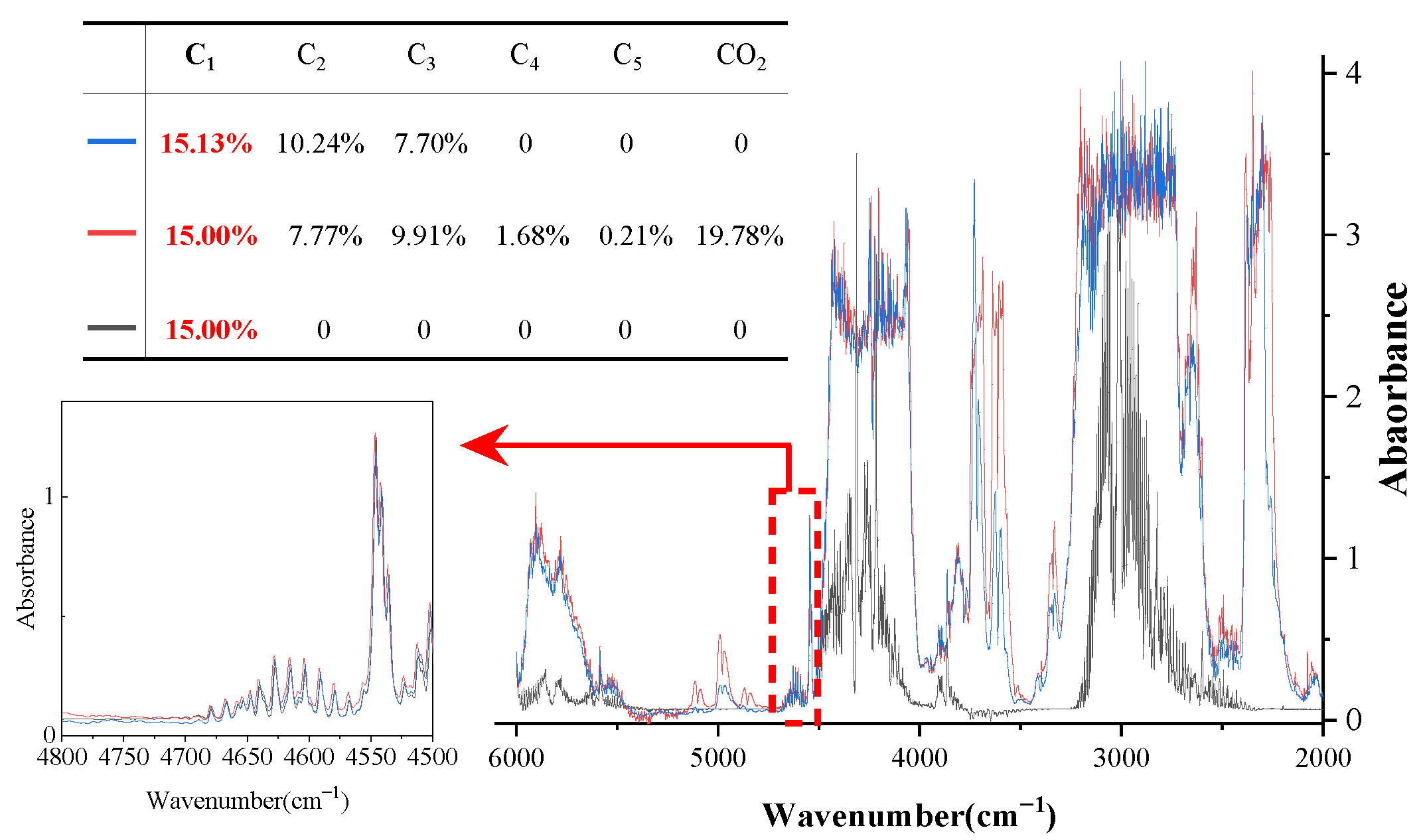
  • Because of the high similarity of the molecular structure of alkane gas, the infrared absorption characteristic peaks are too overlapped to separate in multicomponent gas mixtures;
  • Because of the great uncertainties of the composition of the logging gas and the limited number of samples for modelling, fast modelling technology is becoming more and more urgent with the increment of required spectrum range and spectral resolution for analysis of more and more kinds of gases.
These two reasons make it important to establish an effective quantitative analysis model for IR spectroscopy gas logging. IR spectra possess complex and overlapping absorption bands, so mathematical procedures are needed for turning the spectra into meaningful information. For different types of oil and gas reservoirs, it is necessary to establish multiple quantitative analysis models with different applicability. This will undoubtedly take up more computing resources and increase the hardware burden of the analysis module, resulting in slow modelling speed.
In order to establish a rapid modelling method with good accuracy and to promote the application of infrared spectroscopy gas-logging technology on site, this paper proposes a fast modelling method based on adaptive step-sliding partial least squares (ASS-PLS). Three types of infrared spectrum datasets of logging gas are obtained by mixing six gases of methane (C 1 ), ethane (C 2 ), propane (C 3 ), n-butane (nC 4 ), n-pentane (nC 5 ) and carbon dioxide (CO 2 ). A sliding control function is designed to change the position of the local PLS analysis model in the full spectrum band adaptively, based on the relative change in the current root-mean-square error and the global minimum root-mean-square error for rapid modelling. The experiments are carried out to evaluate the influence of window position and window width on the quantitative analysis accuracy and the performance of the proposed method on the three types of datasets. The results show that the ASS-PLS method proposed in this paper can establish a rapid quantitative analysis model with good accuracy of logging gas, and can meet the actual needs of gas-logging operations.

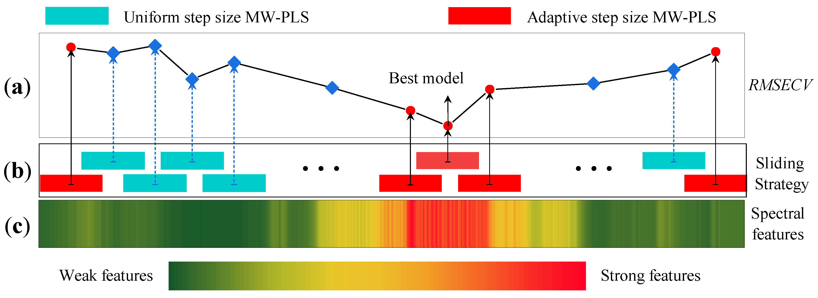
2. Adaptive Step-Sliding Partial Least Squares

2.1. Infrared Quantitative Analysis Principle

Based on Lambert–Beer law [36], the absorption of a certain wavenumber of light by a substance is related to the concentration of the light-absorbing substance and the optical path length, as shown in Figure 1:
The specific relational formula is shown in Equation (1), wherein the absorbance A ( ν ) of the substance with respect to infrared light of a specific frequency is defined as Equation (2), so the relation of Equation (1) can be further expressed as Equation (3):
I ( ν ) = I 0 ( ν ) exp [ σ ( ν ) C L ]
A ( ν ) = lg I ( ν ) I 0 ( ν )
A ( ν ) = σ ( ν ) C L
where ν is the frequency of incident infrared light, I 0 and I are the intensity of incident light and transmitted light, respectively, C is the concentration of the detected target gas, σ ( ν ) is the absorption cross-section of the IR spectrum at frequency ν , and L is the optical path length. For a multicomponent mixed gas with n components, the absorbance satisfies the linear additive property of Equation (4):
A ( ν ) = 1 n A i ( ν ) = 1 n σ i ( ν ) L C i
For the actual spectrum detection in engineering applications, L is known and deter-mined because of the fixed optical path system, and σ i ( ν ) is constant but unknown under one stable pressure, temperature and other physical or chemical environments. Therefore, the characteristic absorption coefficient k ( ν ) in the system can be defined as Equation (5):
k ( ν ) = σ ( ν ) L
Then, the absorbance matrix A and the component concentration matrix C in the mixed system have a linear relationship in Equation (6):
A m × n = k m × p C p × n
where A m × n is the absorbance matrix of n samples at m wavenumber; k m × p is the absorption coefficients of p components at m wavenumber, and C p × n is the concentration of p components in n samples. Generally, the number of target components is much smaller than the number of wavenumber, that means p < < m , so that the solution of the concentration in Equation (6) is a linear, overdetermined, equation-solving problem. Quantitative analysis modelling aims to establish the relationship between absorbance and the concentration of some known samples according to Equation (6), and quantitative analysis aims to obtain the concentration value of an unknown sample according to the established model.

2.2. Partial Least Squares Analysis

Partial least squares is one of the most effective methods to establish the linear relationship between multiple variables in Equation (6). Compared with traditional multiple linear regression, it combines the advantages of principal component regression and canonical correlation analysis, meanwhile it can overcome the problem of much larger sample size than variable dimensionality and the presence of multicollinearity within the variables [37]. Set the absorbance independent variable A and the substance concentration-dependent variable C to E 0 and F 0 , respectively, after data standardization in Equation (7):
E 0 ( i , j ) = A ( i , j ) m e a n ( A ( , j ) ) s t d ( A ( , j ) ) , i = 1 , 2 , , m ; j = 1 , 2 , , n F 0 ( i , j ) = C ( i , j ) m e a n ( C ( , j ) ) s t d ( C ( , j ) ) , i = 1 , 2 , , p ; j = 1 , 2 , , n
where m e a n ( ) is an operator to calculate the average value, s t d ( ) is an operator to calculate the standard deviation, ( i , j ) denotes the element position in a matrix at i-th row j-th column, ( , j ) denotes all elements in the j-th column. Suppose that the first principal components extracted are t 1 and u 1 respectively, and the weight coefficients are w 1 and m 1 respectively. So, t 1 and u 1 are the linear combination of E 0 and F 0 , respectively, t 1 = E 0 w 1 , u 1 = F 0 m 1 . According to the principle of principal components, the variance of t 1 and u 1 is required to be maximized to make the principal components carry more information. According to the canonical correlation analysis, the correlation between t 1 and u 1 is required to be maximized for the best explanation from t 1 to u 1 . Therefore, the covariance of t 1 and u 1 is required to be maximized and the weight coefficients must be unit vectors in Equation (8):
max { C o v ( t 1 , u 1 ) } = max < E 0 w 1 , F 0 m 1 > s . t : w 1 T w 1 = 1 , m 1 T m 1 = 1
This conditional extremum can be solved by the Lagrangian multiplier method to obtain w 1 and m 1 in Equation (9):
L = w 1 T E 0 T F 0 m 1 λ ( w 1 T w 1 1 ) θ ( m 1 T m 1 1 )
where λ and θ are both Lagrange multiplier. By solving Equation (9), the regression equation of E 0 and F 0 to t 1 can be established:
E 0 = t 1 q 1 T + E 1 F 0 = t 1 s 1 T + F 1
where E 1 and F 1 are the residual matrix of the regression equation, q 1 and s 1 are the regression coefficient vectors calculated by the least-square method, q 1 = E 0 T t 1 / ( t 1 T t 1 ) and s 1 = F 0 T t 1 / ( t 1 T t 1 ) .
Furthermore, the second principal components t 2 and u 2 can be obtained by replacing E 0 and F 0 with the residual matrices E 1 and F 1 . If the rank of the A matrix is r, then the calculation will continue, to obtain:
F 0 = t 1 s 1 T + t 2 s 2 T + + t r s r T + F r = E 0 j = 1 r w j T s j T + F r
where F r is the residual matrix when the maximum number of principal components r is extracted. The more principal components extracted, the better the linearity of the model, but the possible overfitting will lead to an unsatisfactory prediction effect.
A leave-one-out cross-validation test is adopted to determine the number of principal components h to be extracted from the spectral data. Each time the i-th spectrum observation data is discarded ( i = 1 , 2 , , n ) , the remaining ( n 1 ) spectrum observation data are used to fit a regression equation with h principal components, and then the discarded i-th spectrum observation data are incorporated into the regression equation to obtain the predicted concentration c ^ ( i ) j ( h ) . The above verification is repeated for i = 1 , 2 , , n . Then, we obtain the sum of squared prediction errors of the j-th concentration-dependent variable ( j = 1 , 2 , , p ) in Equation (12):
S j ( h ) = i = 1 n ( c i j c ^ ( i ) j ( h ) ) 2 , j = 1 , 2 , , p
then, the sum of squares of prediction errors of the concentration C is:
S ( h ) = j = 1 p S j ( h )
In addition, all spectral data are used to fit the regression equation with h principal components again. Defining the predicted value of the i-th spectral data as c ^ i j ( h ) , then the sum of the squared errors of the j-th concentration-dependent variable can be defined as Equation (14):
S j * ( h ) = i = 1 n ( c i j c ^ i j ( h ) ) 2 , j = 1 , 2 , , p
then, the sum of the squared errors of the concentration C is:
S * ( h ) = j = 1 p S S j ( h )
When S ( h ) reaches the minimum value, the corresponding h is the number of all the best principal components. Usually, there is always S ( h ) < S * ( h ) , and S * ( h ) < S * ( h 1 ) at the same time. Define the cross-validity index Q h 2 :
Q h 2 = 1 S ( h ) / S * ( h 1 )
After the principal component extraction process, the cross-validity index is hoped to be as small as possible. The threshold of Q h is always set to 0.05, then S ( h ) / S * ( h 1 ) ( 1 0.05 ) 2 = 0.952 , and it is beneficial to the accuracy by increasing the number of the principal components. Therefore, for the process of extracting the principal components, if Q h 2 0.0975 at the h-th principal component, the model meets the accuracy requirements and stops extracting. Otherwise, the ( h + 1 ) -th principal component extraction should be continued.
As shown in Equation (17), the root-mean-square error (RMSE, RMSECV for model calibration) is adopted as one of the most important evaluation indexes of quantitative methods.
RMSE ( RMSECV ) = i = 1 n ( C i C ^ i ) 2 / n
where C i is the real concentration of the sample, C ^ i is the predicted concentration, and n is the number of predicted samples.

2.3. Adaptive Step Sliding

Due to the uncertainty of the composition of the logging gas, the spectrometer is often required to scan with a wider frequency band. This means that it is necessary to abandon the irrelevant weak absorption and impurity absorption bands to establish a quantitative analysis model with strong robustness and high precision. Further, the similarity of the molecular structure of alkanes results in a continuous distribution of their strong characteristic absorption bands.
As shown in Figure 2b (blue box), the usual strategy is to traverse the whole spectrum with fixed sliding-step size in one search, and to establish the corresponding local model in the moving process to calculate the corresponding RSMECV value; then repeat the above process by changing the window width, and select the window with the minimum RSMECV value as the optimal window to establish the optimal model. This undoubtedly consumes a lot of computing resources and time [38].
Different from the uniform sliding strategy of MW-PLS, the ASS-PLS shown in Figure 2b (red box) can adaptively adjust the step size of each sliding according to the RMSECV value. This strategy can skip the spectral band information with more redundant information (blue dot) to achieve high-efficiency modelling. To this end, this paper designs an adaptive step-sliding control function of Equation (18) to determine the optimal local modelling interval with the best position of the moving window in only one search in the full spectrum. The real-time Δ RMSECV change value input by this function has an obvious nonlinear relationship with the output step size δ . In this way, the window can quickly slide on the weak feature band, and realize fine sliding on the strong feature band, so as to ensure that the window will not skip the ideal modelling interval during the sliding process.
δ = δ 0 + β ( 1 exp ( ( π · Δ RMSECV / ξ ) 2 / 2 ) )
where δ is the moving step size; δ 0 is the basic moving step size, which is a very small constant to avoid the function falling into dead loops when Δ RMSECV = 0 ; β is the maximum offset of the moving step size; ξ is the kernel of the function, denoting the offset degree of Δ RMSECV ; Δ RMSECV is the offset value of real-time RMSECV relative to the minimum RMSECV*, Δ RMSECV = RMSECV RMSECV * , and e x p ( ) is the exponential function.
In ASS-PLS shown by Algorithm 1, when the offset degree of RMSECV is not considered ( ξ ) , the ASS-PLS algorithm degenerates into moving window PLS (MW-PLS) with fixed moving speed.
Algorithm 1: ASS-PLS local modelling algorithm
Energies 15 01325 i001

3. Experiment and Discussion

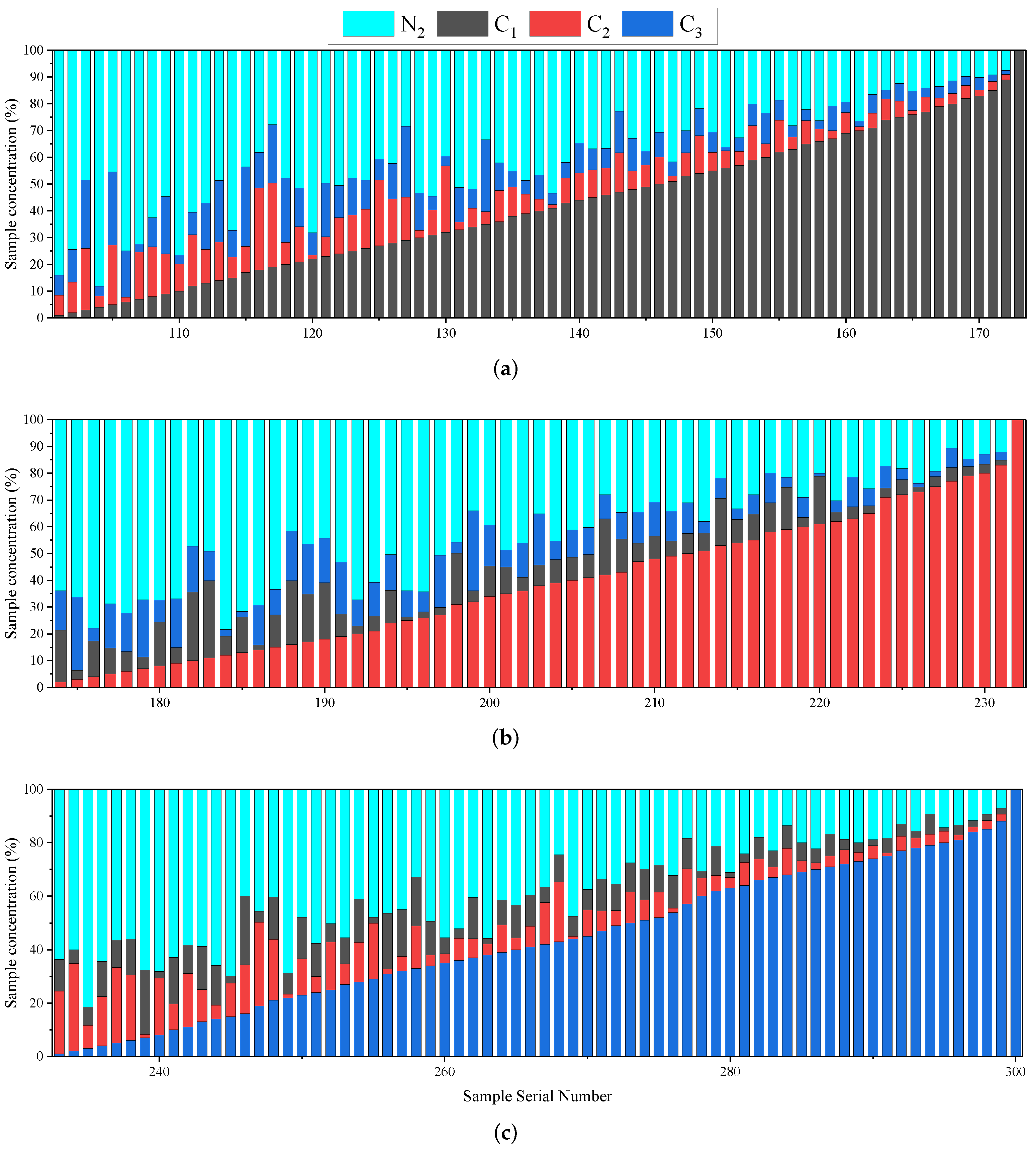
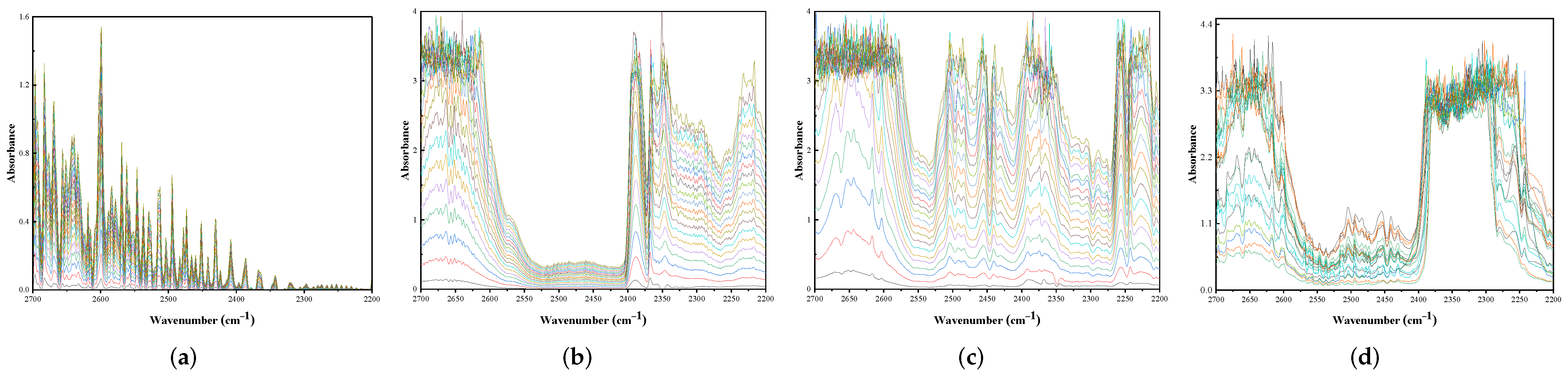
3.1. Experiment Dataset

Three types of spectral datasets are obtained by the designed infrared spectrum data acquisition system, shown in Figure 3. With methane (C 1 , 99.999%), ethane (C 2 , 99.999%), propane (C 3 , 99.999%), n-butane (nC 4 , 4.999%), n-pentane (nC 5 , 3.999%), carbon dioxide (CO 2 , 99.999%) and its mixture as the target gas, the test sample with nitrogen (N 2 , 99.999%) as the carrier gas is fed into the gas-mixing system (LFIX-7000, Laifeng, Chengdu, China), the output error is ±1% of the input concentration), which realizes the mixed gas by controlling the intake flow. After being dehumidified by the drying tube (MD-070-24F-4091119-02, Perma Pure, US), the test sample is introduced into the airtight light path pool with a volume of 400 mL and an effective light range length of 4.8 m (PMG10030, YingSa, Shanghai, China). The internal temperature of the light path pool is kept constant at 27.5 °C by the heat preservation controlled by the temperature controller. Finally, the infrared spectrum data are acquired by the IR spectrometer (ALPHA II, Bruker, Germany) controlled by the computer.
The collection spectral range of the spectrometer is 2000∼6000 cm 1 , the sampling interval is 1.03 cm 1 , and the number of collection points for a single sample is 3882.
The obtained IR spectrum dataset contains 400 samples. The datasets can be divided into three types. The first dataset (one-component dataset, sample serial number 1∼100) consists of one component of six elementary gases C 1 , C 2 , C 3 , nC 4 , nC 5 and CO 2 with the concentration distribution in Table 1. As shown in Figure 4, the second dataset (three-component dataset, sample serial number 101∼300) consists of three components (C 1 , C 2 , C 3 ) with the concentration of one component increasing and the other two random. As shown in Figure 5,the third dataset (six-component dataset, sample serial number 301∼400) consists of six components (C 1 , C 2 , C 3 , nC 4 , nC 5 , CO 2 ) with the concentration random.
Figure 6 shows the spectral curves of part samples (cutting the range of 2200∼2700 cm 1 ). It has a good absorption linearity with the increment of concentration of the samples in one-component dataset. As the number of components increases, the absorption peaks of different components are seriously covered up and overlapped in Figure 6d.

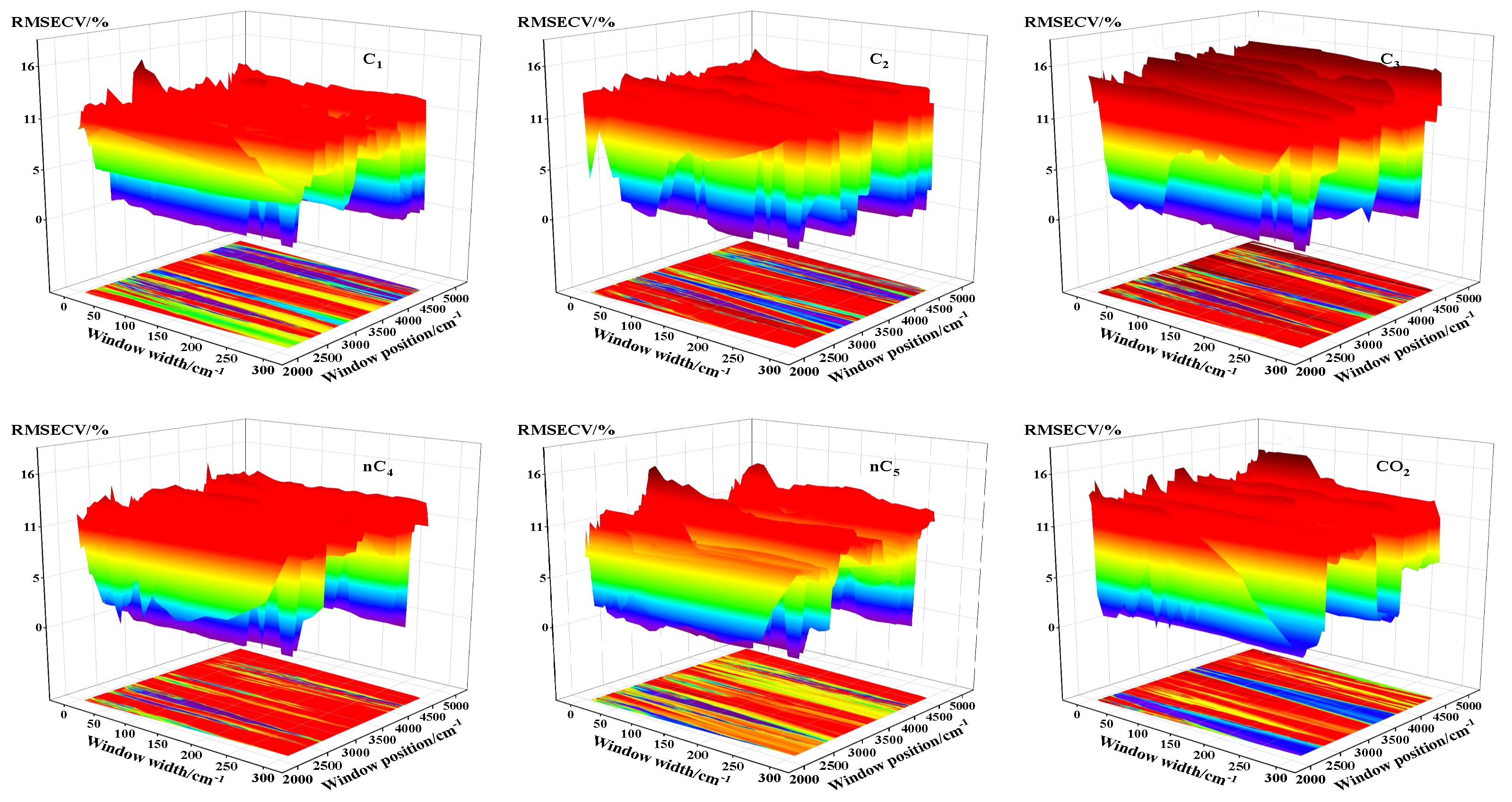
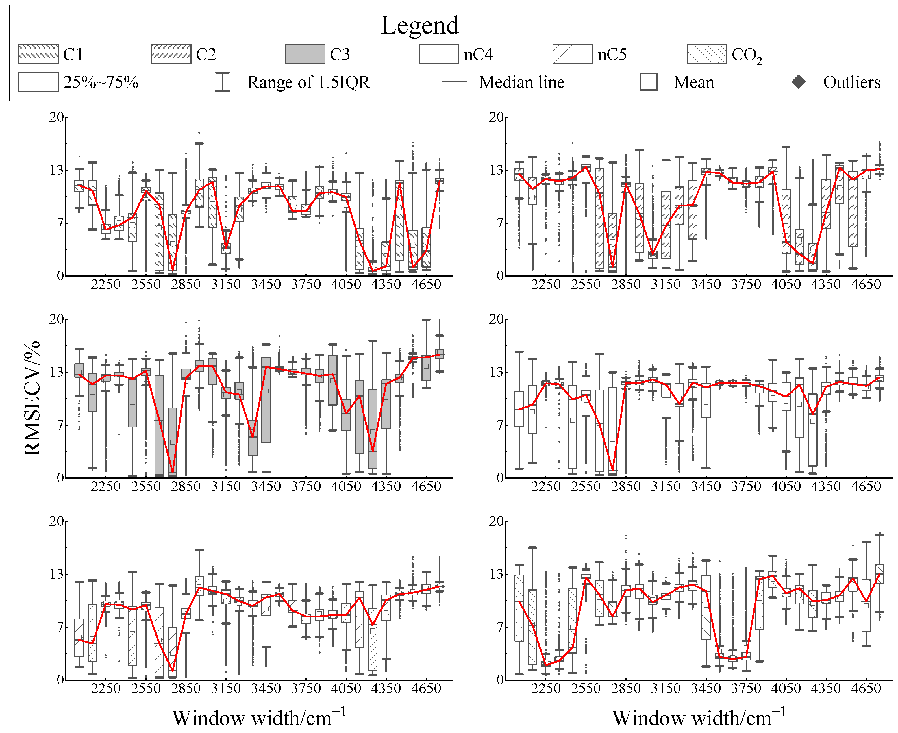
3.2. Influencing Factors on Local Modelling

In this paper, experiments were carried out firstly in the six-component dataset in order to explore the influence of the window width and window position (the centre position of the window is recorded as the position of the window) during the movement of the local modelling window for the six substances. Taking RMSECV as the model evaluation index, Figure 7 shows the effect of the local PLS model under different window positions (2050∼4750 cm 1 , in increments of 100 cm 1 ) and different window widths (5∼300 cm 1 , in increments of 5 cm 1 ).
Conclusions can be obtained from Figure 7 as follow:
  • The RMSECV of different substances are distributed in the range of 0∼16%, and all of them show similar wavelike distribution in the direction of the window position;
  • The RMSECV of the same substance shows obvious stripe distribution on the window position;
  • The stripe distributions of C 1 ∼C 5 are similar, but are obviously different from CO 2 .
This indicates that the influence of the window position is much greater than the influence of the window width in the local PLS modelling; the influence of the window position to C 1 ∼C 5 is alike, but is obviously different from CO 2 , which is determined by the same C-H and C-C chemical bond in C 1 ∼C 5 but the C=O chemical bond in CO 2 .

3.2.1. Influence of the Window Position

In order to further confirm the influence of the window position, the RMSECV distributions of six substances with a window width of 5∼300 cm 1 (in increments of 5 cm 1 ) at 28 different positions (2050∼4750 cm 1 , in increments of 100 cm 1 ) were counted in Figure 8. Each box represents the RMSECV statistics of the local PLS modelling of all different window widths at the specified window position. The average value of each position is connected to observe the change trend (the red solid line in Figure 8).
It can be clearly seen that the influence of the window position fluctuates greatly, and the best window position for modelling of each hydrocarbon substance is around 2750 cm 1 , which is mainly determined by the symmetrical stretching vibration frequency of -CH 3 and -CH 2 [39]. A good quantitative analysis model can be established around 4250 cm 1 in the near infrared band or around 3350 cm 1 in the middle infrared band, but its analytical accuracy decreases greatly as the carbon chain grows from C 1 to C 5 . It no longer has obvious modelling advantages when the carbon chain grows to C 4 . Comparing the performance of the PLS models around 2750 cm 1 , 2650 cm 1 and 2850 cm 1 , it is found that the modelling window position is very important to build an optimal quantitative analysis model.

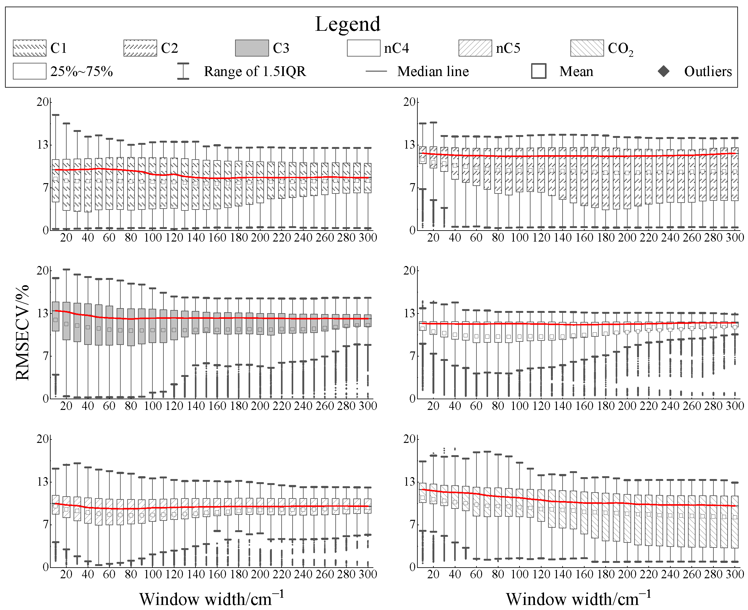
3.2.2. Influence of the Window Width

In order to further confirm the influence of the width, the RMSECV distributions of six substances in the range of 2050∼4750 cm 1 and 30 different widths (10∼300 cm 1 , in increments of 10 cm 1 ) were counted in Figure 9. Similarly, each box represents the RMSECV statistics of the local PLS modelling of all different window positions under the specified width of the window.
Obviously, the mean and median values of each substance changed gently under different window widths. From the change in the range of 25∼75% and 1.5 IQR, the stability of the C 1 ∼C 5 models decreased, but it remained unchanged for CO 2 , when the window width increased gradually. It can be explained that the performance of local models for hydrocarbons may be more easily affected by irrelevant interference information introduced due to too large a window because of the narrow band infrared absorption peak of hydrocarbons. As the length of the molecular carbon chain increases, the range of 1.5 IQR became narrower, further indicating that the search of the window position will become more important than the window width.
Figure 10 shows the IR spectra of three different samples with the same C 1 concentration of 15% and the selected modelling interval of ASS-PLS. Affected by other components, the absorption peaks (around 2750 cm 1 ) of C 1 overlapped badly, which makes it very difficult to build a good quantitative analysis model based on absorption peaks directly. However, the ASS-PLS algorithm proposed in this paper can adaptively find the optimal modelling position (the red dashed box area) free from interference of other components, which is a great improvement for high-precision quantitative analysis of multicomponent mixtures.

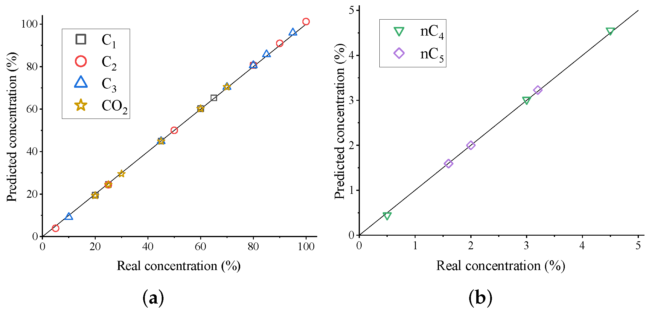
3.3. Quantitative Analysis Results

All the programs are implemented in MATLAB (Ver. R2021a) software with the computer processor Intel(R) Core (TM) i5-9600KF CPU @ 3.70 GHz. Quantitative tests were performed on the three types of datasets. Each dataset was divided into a training set and test set according to a random ratio of 7:3.
Figure 11 shows the correlation between the actual concentration and the predicted concentration of 30 samples in the one-component test set. It can be seen that the prediction accuracy of each substances is the best when the concentration is near 50%, but it starts to show a small degree of deviation toward the two ends gradually. This is probably caused by the instrument error of the mixed gas system in the preparation of experimental samples, which is ±1% of the concentration of the input gas source. However, the ASS-PLS model still has good analysis accuracy within ±0.4% of RMSE for one-component samples.
Figure 12 shows the correlation between the real concentration and the predicted concentration of 60 samples in the three-component dataset and 30 samples the six-component dataset. Compared with the prediction of one-component samples, the quantitative analysis accuracy of mixed components reduced, especially in the low-concentration section. On the one hand, as the number of components increases, the IR characteristic absorption peaks of different substances overlap to varying degrees. On the other hand, the absorption intensity of low-concentration components is small in multicomponent samples, which makes the IR absorption characteristic peaks of low-concentration components more susceptible to noise and other components.
In addition, the actual concentration of CO 2 and the predicted concentration still maintain a good correlation away from the obvious overlap of the infrared characteristic absorption peaks because of the different molecular structure.
The performance of the proposed ASS-PLS method was further compared with full-spectrum PLS (F-PLS, blank contrast group), successive projections algorithm PLS (SPA-PLS), competitive adaptive reweighting sampling PLS (CARS-PLS) and moving window PLS (MW-PLS) by 10 repeated tests in the six-component dataset. Figure 13 shows the performance of the five models.
It can be seen that the stability and accuracy of ASS-PLS and MW-PLS models are significantly better than the other three modelling methods, while the performance of F-PLS modelling is extremely poor. In addition, the prediction accuracy of CO 2 is always higher than that of the other five components, which also verifies that the prediction accuracy of hydrocarbons has been affected by the overlapping infrared absorption due to the similar molecular structure. The bolded text indicates the best prediction.
According to the RSME values in Table 2, the prediction accuracy in the one-component dataset is much higher than that in the multicomponent dataset for the same substance by the same quantitative analysis method, indicating that it is more difficult to establish a good quantitative analysis model for multicomponent mixtures. It is noticeable that the prediction accuracy of CO 2 has a smaller reduction in the multicomponent dataset because the characteristic infrared absorption band of CO 2 is not obviously affected with the increased number of hydrocarbon components. Furthermore, the prediction accuracy of ASS-PLS model is slightly better than the MW-PLS model, and significantly better than the CARS-PLS and SPA-PLS models.
It is extremely necessary to realize rapid modelling of quantitative analysis models in completely unknown application sites to promote the application of IR spectroscopy gas logging. Table 3 shows the number of wavenumber variables extracted by the modelling algorithm, analysis time and the modelling time (with the Q h of PLS in (16) is 0.05) of the several algorithm models mentioned above in the six-component dataset.
Since the analysis time is small enough, the difference in the analysis time is almost negligible for practical applications. In addition to the higher model accuracy, the smaller modelling time will become more practical to update the model in time. Even CARS-PLS and SPA-PLS have a smaller modelling time, but the stabilities of the models are insufficient (shown in Figure 13) because of the less wavenumber variables extracted. Even MW-PLS and ASS-PLS have better prediction accuracy (shown in Table 2), but the modelling time of MW-PLS is nearly 349 times that of ASS-PLS due to lots of meaningless repetitions.
Experiments show that ASS-PLS has ideal modelling time with good prediction accuracy. Therefore, the robust accuracy and high-efficiency modelling of the ASS-PLS model is significantly more in line with the requirements of gas-logging applications for high stability, high precision and fast analysis.

4. Conclusions

This paper proposes a new ASS-PLS infrared spectroscopy gas-logging modelling method. The algorithm searches for the optimal quantitative analysis modelling interval of each component of mixtures in the full spectrum by sliding a window determined by an adaptive step-sliding control function. Three types of infrared datasets for the logging gas are constructed in this paper. Based on the datasets, it has been analysed that the ASS-PLS method can adaptively determine an optimal modelling interval within 2000∼6000 cm 1 of infrared data. Comparative experiments show that the stability, speed and accuracy of ASS-PLS modelling are better than those of the other four modelling methods. In addition, the experimental results in different mixed types of samples also show that the gas-logging technology realized by infrared spectroscopy has the following distinct unique features compared with other industrial applications.
  • The infrared characteristic distribution of logging gas has an obvious concentration, and the local modelling strategy of continuous interception can effectively retain the characteristic information and improve the prediction accuracy and stability of the model.
  • The accuracy of the local model under the continuous interception strategy is much more sensitive to the modelling position than the interception width.
  • The similarity of the alkane molecular structure can lead to a shift in the optimal modelling interval under different mixing types.
The proposed ASS-PLS modelling method can fit the above characteristics very well, and is helpful for improving IR spectroscopy gas-logging technology, and it will also have a great contribution to other molecular spectroscopy analyses with high similarity.

Author Contributions

Conceptualization, Z.L. and W.P.; methodology, Z.L.; software, W.P.; validation, Z.L., W.P., H.D. and C.J.; formal analysis, Z.L. and G.C.; investigation, Z.L. and H.L.; resources, H.L.; data curation, W.P.; writing—original draft preparation, W.P.; writing—review and editing, Z.L. and G.C.; visualization, W.P.; supervision, H.L.; project administration, H.L.; funding acquisition, H.L. All authors have read and agreed to the published version of the manuscript.

Funding

This work is supported in part by the National Natural Science Foundation of China (52074233), the Science and the Technology Cooperation Project of the China National Petroleum Corporation and Southwest Petroleum University Innovation Alliance (2020CX040000).

Institutional Review Board Statement

Not applicable.

Informed Consent Statement

Not applicable.

Data Availability Statement

Not applicable.

Acknowledgments

The authors would like to acknowledge the National Natural Science Foundation of China (52074233), the Science and Technology Cooperation Project of the China National Petroleum Corporation and Southwest Petroleum University Innovation Alliance (2020CX040000) and ChinaFrance Bohai Geoservices Co., Ltd. (CFB_TG_TI_2019_012). The contents of this paper are solely the authors’ responsibility and not to be taken as the official views of any of the organizations listed above.

Conflicts of Interest

The authors declare no conflict of interest.

References

  1. Ighodalo, E.; Davies, G.; D’Souza, S.A.; Ahmed, A. Increasing Certainty in Formation Evaluation Utilizing Advanced Mud Logging Gas Analysis. In Proceedings of the SPE Kingdom of Saudi Arabia Annual Technical Symposium and Exhibition, Dammam, Saudi Arabia, 25 April 2017. [Google Scholar] [CrossRef]
  2. Ferroni, G.; Rivolta, F.; Schifano, R. Improved Formation Evaluation While Drilling With a New Heavy Gas Detector. In Proceedings of the Society of Professional Well Log Analysts Annual Logging Symposium, Cartagena, Colombia, 16–20 June 2012. [Google Scholar]
  3. Zakrevskiy, K.E.; Gazizov, R.K.; Ryzhikov, E.A.; Freydin, K.V. Consistency evaluation technology for automatic well-log correlation using well logging data (Russian). Neft. Khozyaystvo Oil Ind. 2021, 2021, 22–26. [Google Scholar] [CrossRef]
  4. Kandel, D.; Quagliaroli, R.; Segalini, G.; Barraud, B. Improved Integrated Reservoir Interpretation Using Gas While Drilling Data. SPE Reserv. Eval. Eng. 2001, 4, 489–501. [Google Scholar] [CrossRef]
  5. Kriel, W.; Spence, A.; Kolodziej, E.; Hoolahan, S. Improved Gas Chromatographic Analysis of Reservoir Gas and Condensate Samples. In Proceedings of the SPE International Conference on Oilfield Chemistry, New Orleans, LA, USA, 2–5 March 1993. [Google Scholar] [CrossRef]
  6. Breviere, J.; Herzaft, B.; Mueller, N. Gas Chromatography—Mass Spectrometry (Gcms)—A New Wellsite Tool For Continuous C1-C8 Gas Measurement In Drilling Mud—Including Original Gas Extractor And Gas Line Concepts. First Results And Potential. In Proceedings of the Society of Professional Well Log Analysts 43rd Annual Logging Symposium, Oiso, Japan, 2–5 June 2002. [Google Scholar]
  7. Brumboiu, A.; Hawker, D.; Norquay, D.; Law, D. Advances in Chromatographic Analysis of Hydrocarbon Gases in Drilling Fluids? The Application of Semi-Permeable Membrane Technology to High Speed TCD Gas Chromatography. In Proceedings of the Society of Professional Well Log Analysts 46th Annual Logging Symposium, New Orleans, LA, USA, 22–26 June 2005. [Google Scholar]
  8. Cramers, C.A.; Janssen, H.G.; van Deursen, M.M.; Leclercq, P.A. High-speed gas chromatography: An overview of various concepts. J. Chromatogr. A 1999, 856, 315–329. [Google Scholar] [CrossRef]
  9. Agah, M.; Lambertus, G.; Sacks, R.; Wise, K. High-Speed MEMS-Based Gas Chromatography. J. Microelectromech. Syst. 2006, 15, 1371–1378. [Google Scholar] [CrossRef]
  10. Rowe, M.; Splapikas, T. Jumping Mass Spectrometer. In Proceedings of the SPE Kingdom of Saudi Arabia Annual Technical Symposium and Exhibition, Dammam, Saudi Arabia, 23–26 April 2017. [Google Scholar] [CrossRef]
  11. Rowe, M.; Muirhead, D. Mud-Gas Extractor and Detector Comparison. In Proceedings of the SPE Kingdom of Saudi Arabia Annual Technical Symposium and Exhibition, Dammam, Saudi Arabia, 23–26 April 2017. [Google Scholar] [CrossRef]
  12. Sauer, C.; Lorén, A.; Schaefer, A.; Carlsson, P.A. On-Line Composition Analysis of Complex Hydrocarbon Streams by Time-Resolved Fourier Transform Infrared Spectroscopy and Ion–Molecule Reaction Mass Spectrometry. Anal. Chem. 2021, 93, 13187–13195. [Google Scholar] [CrossRef] [PubMed]
  13. van der Veen, A.M.H.; Nieuwenkamp, G.; Zalewska, E.T.; Li, J.; de Krom, I.; Persijn, S.; Meuzelaar, H. Advances in metrology for energy-containing gases and emerging demands. Metrologia 2020, 58, 012001. [Google Scholar] [CrossRef]
  14. Diller, D.E.; Chang, R.F. Composition of Mixtures of Natural Gas Components Determined by Raman Spectrometry. Appl. Spectrosc. 1980, 34, 411–414. [Google Scholar] [CrossRef]
  15. Kosacki, I.; Srinivasan, S. Application of Raman Spectroscopy for Hydrocarbon Characterization. In Proceedings of the Nace Corrosion 2017, New Orleans, LA, USA, 26–30 March 2017. [Google Scholar]
  16. Sharma, R.; Poonacha, S.; Bekal, A.; Vartak, S.; Weling, A.; Tilak, V.; Mitra, C. Raman analyzer for sensitive natural gas composition analysis. Opt. Eng. 2016, 55, 1–8. [Google Scholar] [CrossRef]
  17. Rathmell, C. Data-Driven Raman Spectroscopy in Oil and Gas: Rapid Online Analysis of Complex Gas Mixtures. Spectrosc. Suppl. 2018, 33, 34–42. [Google Scholar]
  18. Livanos, G.; Zervakis, M.; Pasadakis, N.; Karelioti, M.; Giakos, G. Deconvolution of petroleum mixtures using mid-FTIR analysis and non-negative matrix factorization. Meas. Sci. Technol. 2016, 27, 114005. [Google Scholar] [CrossRef]
  19. Sell, J.K.; Jakoby, B. A simple mid-infrared measurement system based on a tunable filter for the analysis of ternary gas mixtures. Meas. Sci. Technol. 2013, 24, 084006. [Google Scholar] [CrossRef]
  20. Indo, K.; Hsu, K.; Pop, J. Estimation of Fluid Composition From Downhole Optical Spectrometry. SPE J. 2015, 20, 1326–1338. [Google Scholar] [CrossRef]
  21. Piazza, R.; Vieira, A.; Sacorague, L.A.; Jones, C.; Dai, B.; Pearl, M.; Aguiar, H. Real-Time Downhole MID-IR Measurement of Carbon Dioxide Content. In Proceedings of the Society of Professional Well Log Analysts 60th Annual Logging Symposium, The Woodlands, TX, USA, 15–19 June 2019. [Google Scholar] [CrossRef]
  22. Ren, Q.; Chen, C.; Wang, Y.; Li, C.; Wang, Y. A Prototype of ppbv-Level Midinfrared CO2 Sensor for Potential Application in Deep-Sea Natural Gas Hydrate Exploration. IEEE Trans. Instrum. Meas. 2020, 69, 7200–7208. [Google Scholar] [CrossRef]
  23. Moro, M.K.; dos Santos, F.D.; Folli, G.S.; Romão, W.; Filgueiras, P.R. A review of chemometrics models to predict crude oil properties from nuclear magnetic resonance and infrared spectroscopy. Fuel 2021, 303, 121283. [Google Scholar] [CrossRef]
  24. Kamboj, U.; Kaushal, N.; Jabeen, S. Near Infrared Spectroscopy as an efficient tool for the Qualitative and Quantitative Determination of Sugar Adulteration in Milk. J. Phys. Conf. Ser. 2020, 1531, 012024. [Google Scholar] [CrossRef]
  25. Gao, Q.; Wang, M.; Guo, Y.; Zhao, X.; He, D. Comparative Analysis of Non-Destructive Prediction Model of Soluble Solids Content for Malus micromalus Makino Based on Near-Infrared Spectroscopy. IEEE Access 2019, 7, 128064–128075. [Google Scholar] [CrossRef]
  26. Sun, J.; Yang, W.; Feng, M.; Liu, Q.; Kubar, M.S. An efficient variable selection method based on random frog for the multivariate calibration of NIR spectra. RSC Adv. 2020, 10, 16245–16253. [Google Scholar] [CrossRef] [Green Version]
  27. Galvão, R.K.H.; Araújo, M.C.U.; Fragoso, W.D.; Silva, E.C.; José, G.E.; Soares, S.F.C.; Paiva, H.M. A variable elimination method to improve the parsimony of MLR models using the successive projections algorithm. Chemom. Intell. Lab. Syst. 2008, 92, 83–91. [Google Scholar] [CrossRef]
  28. Yu, Y.; Huang, J.; Zhu, J.; Liang, S. An Accurate Noninvasive Blood Glucose Measurement System Using Portable Near-Infrared Spectrometer and Transfer Learning Framework. IEEE Sens. J. 2021, 21, 3506–3519. [Google Scholar] [CrossRef]
  29. Wang, J.; Lu, S.; Wang, S.H.; Zhang, Y.D. A review on extreme learning machine. Multimed. Tools Appl. 2021. [Google Scholar] [CrossRef]
  30. Jiang, H.; Liu, G.; Mei, C.; Yu, S.; Xiao, X.; Ding, Y. Measurement of process variables in solid-state fermentation of wheat straw using FT-NIR spectroscopy and synergy interval PLS algorithm. Spectrochim. Acta Part A Mol. Biomol. Spectrosc. 2012, 97, 277–283. [Google Scholar] [CrossRef] [PubMed]
  31. Yu, H.; Du, W.; Lang, Z.Q.; Wang, K.; Long, J. A Novel Integrated Approach to Characterization of Petroleum Naphtha Properties From Near-Infrared Spectroscopy. IEEE Trans. Instrum. Meas. 2021, 70, 1–13. [Google Scholar] [CrossRef]
  32. Ouyang, T.; Wang, C.; Yu, Z.; Stach, R.; Mizaikoff, B.; Huang, G.B.; Wang, Q.J. NOx Measurements in Vehicle Exhaust Using Advanced Deep ELM Networks. IEEE Trans. Instrum. Meas. 2021, 70, 1–10. [Google Scholar] [CrossRef]
  33. Liu, L.; Yan, L.; Xie, Y.; Xia, G. Content measurement of textile mixture by near infrared spectroscopy based on BP neural network. In Proceedings of the 2010 3rd International Congress on Image and Signal Processing, CISP 2010, Yantai, China, 16–18 October 2010; Volume 7, pp. 3354–3358. [Google Scholar] [CrossRef]
  34. Li, Y.; Zhang, Y.; Zhang, W.B.; Xu, Y.Y.; Zhang, G.J. Comparative study of partial least squares and neural network models of near-infrared spectroscopy for aging condition assessment of insulating paper. Meas. Sci. Technol. 2020, 31, 045501. [Google Scholar] [CrossRef]
  35. Kumar, K. Competitive adaptive reweighted sampling assisted partial least square analysis of excitation-emission matrix fluorescence spectroscopic data sets of certain polycyclic aromatic hydrocarbons. Spectrochim. Acta Part A Mol. Biomol. Spectrosc. 2021, 244, 118874. [Google Scholar] [CrossRef]
  36. Huang, G.; He, J.; Zhang, X.; Feng, M.; Tan, Y.; Lv, C.; Huang, H.; Jin, Z. Applications of Lambert-Beer law in the preparation and performance evaluation of graphene modified asphalt. Constr. Build. Mater. 2021, 273, 121582. [Google Scholar] [CrossRef]
  37. Silalahi, D.D.; Midi, H.; Arasan, J.; Mustafa, M.S.; Caliman, J.P. Kernel partial diagnostic robust potential to handle high-dimensional and irregular data space on near infrared spectral data. Heliyon 2020, 6, e03176. [Google Scholar] [CrossRef]
  38. Jiang, W.; Lu, C.; Zhang, Y.; Ju, W.; Wang, J.; Hong, F.; Wang, T.; Ou, C. Moving-Window-Improved Monte Carlo Uninformative Variable Elimination Combining Successive Projections Algorithm for Near-Infrared Spectroscopy (NIRS). J. Spectrosc. 2020, 6, 3590301. [Google Scholar] [CrossRef]
  39. Kazansky, V.B.; Subbotina, I.R.; Jentoft, F.C.; Schlögl, R. Intensities of C-H IR Stretching Bands of Ethane and Propane Adsorbed by Zeolites as a New Spectral Criterion of Their Chemical Activation via Polarization Resulting from Stretching of Chemical Bonds. J. Phys. Chem. B 2006, 110, 17468–17477. [Google Scholar] [CrossRef]
Figure 1. Schematic diagram of Lambert–Beer law.
Energies 15 01325 g001
Figure 2. Process diagram of sliding window local modelling strategy: (a) RMSECV values during the sliding window. Red dots indicate ASS-PLS and blue dots indicate MW-PLS. (b) Window position for local modelling. (c) Analyse characteristic intensities of spectral bands.
Energies 15 01325 g002
Figure 3. IR spectrum acquisition system. (a) Schematic diagram of collection process. (b) The actual hardware structure of gas-logging instrument.
Energies 15 01325 g003
Figure 4. The concentration value of each sample in the three-component dataset. The horizontal axis represents the sample index number, and the vertical axis represents the sample concentration. (a) C 1 increments. (b) C 2 increments. (c) C 3 increments.
Energies 15 01325 g004
Figure 5. The concentration value of each sample in the six-component dataset.
Energies 15 01325 g005
Figure 6. Spectral curve of the sample of the IR spectrum dataset. (a) Sample serial number 1∼20 (C 1 ). (b) Sample serial number 21∼40 (C 2 ). (c) Sample serial number 41∼60 (C 3 ). (d) Sample serial number 101∼120 (mixed dataset).
Energies 15 01325 g006
Figure 7. The accuracy of the local PLS model is affected by the width and position of the window.
Energies 15 01325 g007
Figure 8. The influence of the local modelling position on the quantitative analysis model of six substances. The statistics include the range of 25% to 75%, the range of 1.5 times the interquartile range (1.5 IQR), the median, mean value and abnormal value (outliers).
Energies 15 01325 g008
Figure 9. The influence of local modelling width on the quantitative analysis model of six substances.
Energies 15 01325 g009
Figure 10. The IR spectra of three different samples with the same concentration of C 1 and the modelling interval selected by ASS-PLS (the red dotted box). The black line represents a sample in the one-component dataset. The red line represents a sample in the three-component dataset. The blue line represents a sample in the six-component dataset.
Energies 15 01325 g010
Figure 11. The correlation between the actual concentration and the predicted concentration of samples in the one-component test set. The horizontal axis is the real concentration, and the vertical axis is the predicted concentration of ASS-PLS model, the black line means predicted concentration equal to real concentration. (a) Prediction of C 1 , C 2 , C 3 and CO 2 . (b) Prediction of nC 4 and nC 5 .
Energies 15 01325 g011
Figure 12. Prediction results in three-component dataset and six-component. (a) Prediction of the three-component dataset. (b) Prediction of the six-component dataset.
Energies 15 01325 g012
Figure 13. The performance of five different quantitative analysis methods for 10 repeated tests in the six-component dataset. The horizontal axis represents the number of repeated tests, and the vertical axis represents the model accuracy by RMSE.
Energies 15 01325 g013
Table 1. Standard concentration and sample concentration distribution of the one-component dataset.
SubstanceStandard Gas ConcentrationConcentration GradientSample Index Number
C 1 99.999%5%1∼20
C 2 21∼40
C 3 41∼60
CO 2 61∼80
nC 4 4.999%0.5%81∼90
nC 5 3.999%0.4%91∼100
Table 2. Comparison of the effects of five different analysis methods in three types of datasets.
SubstanceDatasetRMSE (%)
F-PLSCARS-PLSSPA-PLSMW-PLSASS-PLS
C 1 A 13.86900.87721.01510.49020.3586
B 27.52543.32541.38511.17431.1628
C 310.73043.86981.87501.97421.5020
C 2 A3.68311.45821.30800.77360.5228
B7.21511.65261.89510.94141.4882
C10.78261.23292.13401.66831.3673
C 3 A5.02271.57651.68620.58160.7659
B8.77541.79512.26511.11511.2864
C12.21412.37783.99251.61141.5182
nC 4 A7.22560.79461.27730.20260.1930
C11.65576.46145.52241.76231.4150
nC 5 A5.87460.29650.11370.15840.1874
C9.65204.11985.65411.43861.5524
CO 2 A4.21370.22370.09630.12360.1731
C4.93880.70070.66760.31520.2897
1 A is the one-component test set; 2 B is the three-component test set; 3 C is the six-component test set.
Table 3. Comparison of the number of wavenumber variables extracted, analysis time and the modelling time of several algorithm models in the six-component dataset.
Model ( Q h = 0.05)Wavenumber VariablesAnalysis Time (s)Modelling Time (s)
F-PLS38820.020841.2200
CARS-PLS560.005632.6267
SPA-PLS270.003327.2036
ASS-PLS1000.004732.7247
MW-PLS1000.004311,443.6870
Publisher’s Note: MDPI stays neutral with regard to jurisdictional claims in published maps and institutional affiliations.

