Article

Supporting Decarbonization Strategies of Local Energy Systems by De-Risking Investments in Renewables: A Case Study on Pantelleria Island

by
Riccardo Novo
1,2,3,*,
Francesco Demetrio Minuto
1,4,
Giovanni Bracco
2,3,
Giuliana Mattiazzo
1,2,3,
Romano Borchiellini
1,4 and
Andrea Lanzini
1,4
1
Energy Center Lab, Politecnico di Torino, Corso Duca degli Abruzzi, 24, 10129 Torino, Italy
2
MOREnergy Lab, Politecnico di Torino, Corso Duca degli Abruzzi, 24, 10129 Torino, Italy
3
Dipartimento di Ingegneria Meccanica e Aerospaziale, Politecnico di Torino, Corso Duca degli Abruzzi, 24, 10129 Torino, Italy
4
Dipartimento Energia “Galileo Ferraris”, Politecnico di Torino, Corso Duca degli Abruzzi, 24, 10129 Torino, Italy
*
Author to whom correspondence should be addressed.
Energies 2022, 15(3), 1103; https://doi.org/10.3390/en15031103
Submission received: 11 January 2022 / Revised: 23 January 2022 / Accepted: 27 January 2022 / Published: 2 February 2022
(This article belongs to the Special Issue Optimal Investment Analysis of Renewable Energy)

Abstract

:
Nowadays, energy policymakers are asked to develop strategies to ensure an affordable clean energy supply as well as minimizing investment risks. In addition, the rise of several community engagement schemes and the uptake of user-scale technologies introduce uncertainties that may result in a disruptive factor for energy systems evolution. This paper introduces a novel scenario analysis approach for local energy planning that supports policymakers and investors in prioritizing new renewable power plant investments, addressing the risks deriving from citizens’ choices. Specifically, a combined analysis is performed on the adoption trends of distributed photovoltaic systems and electric vehicles that are expected to heavily influence the evolution of energy systems. For this reason, an energy model is developed for Pantelleria island, and its transition from an oil-based energy supply to a renewable one up to 2050 is investigated. It is demonstrated how optimal-cost renewable-based scenarios can assure a 45% to 52% CO2 emissions reduction and a 6% to 15% overall cost reduction with respect to the diesel-based business-as-usual scenario. The analyzed scenarios disclose the recommended investments in each renewable technology, considering their learning curves and the unpredictability of user-scale technology adoption. Consequently, priorities in the installation of renewable power plants are stressed, starting with the most resilient to future uncertainties, as well as promoting specific incentive measures for citizens’ commitment at a local scale.

1. Introduction

The decarbonization of energy systems is urgent for global warming and represents a key goal of great common interest. Energy policymakers face a complex problem nowadays, as they must combine the achievement of challenging decarbonization targets to guarantee cheap energy supply with the de-risking of investments in renewables [1]. Their task is made difficult, among other things, by the multiple schemes of community engagement in the energy transition process [2], whose implications on a large uptake are still uncertain. The scope of this work is to support decision makers in long-term local energy planning under the uncertainties related to citizens’ commitment and direct participation in the transition process [3]. The target is the planning towards the energy independence of islands, which are ideal environments for implementing specific supporting schemes at a local level [4,5].

1.1. Literature Review

Long-term energy planning emerged during the oil crises of the 1970s when the price volatility of fossil fuels encouraged national and international bodies to decrease energy dependency from abroad through model-supported energy strategies [6]. The environmental concerns are currently the main drivers for studying energy systems’ evolution on a large time scale. Although national and regional supporting policies are essential, local authorities are recognized as critical players in the decarbonization process and, more generally, in the sustainable development path [7]. A strong commitment of local authorities in defining the main actions to push the energy transition is desirable to meet the real territorial needs, enhance communication, and limit the emergence of conflicts [8]. More specifically, the energy planning of isolated areas is needed for driving the development and decarbonization of thousands of islands and remote areas that are highly dependent on the import of fossil fuels or have limited access to energy [9]. In addition, advances in the relative supporting models and methodologies can be crucial for the policymaking towards the local energy autonomy of interconnected areas, representing a topic of increasing importance for ensuring a fully sustainable energy supply [10]. In addition, there is a need to identify priorities in terms of environmental policies [11]. The following literature review presents and classifies the different types of modelling frameworks and tools to support energy planning, focusing on their applicability at a local scale.
There are many energy system models to support energy, environmental, and climate change policy strategies. The first classification of models can be performed according to the approach they use in describing energy systems. The top-down approach generally follows an aggregated view and focuses on macroeconomic relationships as the influence of prices and overall financial markets on the energy system evolution. On the other hand, the bottom-up approach stresses the energy sector’s technical characteristics, ensuring a detailed technological description [12,13]. Although several hybrids exist, two main underlying methodologies within the bottom-up approach can be identified, depending on whether investments in the energy system are exogenous or endogenous [14]. The former includes simulation models that predict the system operation or evolution based on relationships, rules, and equations [15]; such models can also include utility functions and algorithms to describe the energy market. The latter includes optimization models that mainly focus on the evolution of the energy system to prescribe investment strategies, according to techno-economic criteria [16]. This paper focuses on bottom-up optimization models, which deal with endogenous investments and are better suited for recommending the long-term evolution of energy systems.
Several optimization techniques are available to modelers. Most models make use of Linear Programming (LP) or Mixed-Integer Linear Programming (MILP) techniques that consist of an objective function and a set of constraints (equations and inequalities); the difference between the two is in the possible forcing of some variables to be integrated [13]. Other techniques are based on heuristic optimization and non-linear programming. For this work, LP/MILP-based modeling techniques are used, which are the most diffused and generally have acceptable computational burdens even for simulation periods of several decades. Various LP/MILP-based long-term techno-economic optimization modeling tools are used in the academy and at different governmental levels. Among the most widespread, it is worth mentioning MARKAL [17], EFOM [18], their descendant TIMES [19], Balmorel [20], MESSAGE [21], and OSeMOSYS [22,23]. The main distinction criteria among the available modeling tools are: (i) the spatial representation and the flexibility in its definition; (ii) the temporal representation and the flexibility in its definition; (iii) the specific objective function that varies from the maximization of social welfare to a more direct minimization of the energy system discounted cost; and (iv) the type of final service demand, which may be elastic or inelastic, leading to different points of view on the energy market.
Most of the modeling tools mentioned above were primarily applied at the national or transnational level and employed at the local scale in urban and rural energy systems. Cosmi et al. [24] applied MARKAL to study the feasibility of introducing renewable technologies in a Southern Italian urban area, identify the most promising technologies, and estimate their main economic and environmental benefits, as well as the key obstacles for their diffusion. Comodi et al. [25] used TIMES to study the savings from energy efficiency policies at a municipal scale, focusing on the public sector, households, and transport to prioritize local policymakers’ actions. Howells et al. [26] employed TIMES to explore different clean development scenarios for an isolated village in South Africa, demonstrated the environmental benefits of connection to the national electricity grid, and found in the extremely low cost of wood fuel a major limiting factor for the uptake of electricity and Liquified Petroleum Gas (LPG). Fuso Nerini et al. [27] implemented an OSeMOSYS model of a village in Southeast Asia to explore different tiers of energy access and electrification, highlighting the high costs related to the most ambitious goals and suggesting the grid connection as a viable option over a certain level of electricity access. Timmons et al. [28] applied OSeMOSYS to study the cost-effectiveness of different high Renewable Energy Sources (RES) penetration scenarios in the island country Mauritius, identified the 80% RES scenario as the least-cost, and suggested the establishment of a new bagasse-bioethanol-solar-wind renewable energy industry. In addition, Riva et al. [29] linked an OSeMOSYS-based optimization model with an energy consumption projection model based on socioeconomic indicators and a stochastic load profile generator for an application in rural India: researchers pointed out the importance of such an integrated approach for rural developing areas, where energy demand is expected to have a considerable increase.
It has been observed how several long-term optimization modeling tools have been used for different scopes, even at the local and rural levels. In choosing the most appropriate modeling tool for exploring the long-term energy scenarios of isolated areas, it is worth mentioning that commodity demand at a local scale does not strongly influence its market price [30]. Thus, local energy systems can be considered price takers of the national ones, as they have minimal impact on the final users’ overall commodity cost. When dealing with energy systems of limited spatial extension, such as those of municipalities or remote areas, it may thus be sufficient to make use of tools that adopt inelastic—or entirely exogenous—service demands, as OSeMOSYS does.

1.2. Gaps and Contributions

One of the gaps in LP/MILP-based long-term energy models is related to the models’ weakness in accurately assessing the reliability and security of high Variable Renewable Energy Sources (V-RES) penetration in future energy systems [31]. Indeed, the need to study the evolution of energy systems over tens of years requires the use of representative time periods of several hours length, thus renouncing to describe energy systems’ short-term dynamics. This can lead to an overestimation of optimal V-RES capacity and to an underestimation of the needed dispatchable generation; the effect is also greater in energy islands, where flexibility is limited and no connection with back-up grids is available. In this view, Pavičević et al. [32] soft-linked a long-term energy model with a 30-min time-step optimal dispatch model, ensuring the feasibility of the proposed scenarios and studying the flexibility potentials in each demand sector. However, despite the reliability of the resulting outcomes, such an approach requires considerable modelling and computational efforts, with limited potential for wide-spread application at the local energy planning scale.
A further need in energy models is related to the inclusion of future uncertainties in the main model inputs [33] to highlight the reliability of the obtained outcomes and identify the actions to be implemented independently of the evolution of high-level dynamics. In this regard, Leibowicz [34] proposed the use of stochastic programming to support decision making on carbon taxes; Dreier et al. [35] successfully developed an empirical deterministic-stochastic modeling approach, enabling the use of large real-world datasets for prescribing future energy scenarios; Guevara et al. [36] introduced a machine learning framework to overcome uncertainties in strategic investment for national energy systems. Nevertheless, although future uncertainties should also be included in local energy plans, large datasets are not always available on a local scale.
Great interest arises from the uncertainties related to community engagement and the uptake of energy technologies at the consumers’ premises, which could represent a potentially disruptive factor in the evolution of energy systems. Researchers have so far focused on the large-scale impacts of such factors. Gernaat et al. [37] have estimated the global economic potential of rooftop PV that can lead to an 80% increase in the total PV share by 2050. Krause at al. [38] have studied the effect of electric vehicles (EV) diffusion, forecasting a 30% increase in EU electricity consumption in a road transportation high electrification scenario. However, it is necessary to correlate trends in user-scale technology adoption with the optimal long-run evolution of energy systems to support the implementation of targeted energy policies.
The main objective of this paper is to highlight the importance to identify prioritized local energy policy measures, considering the uncertainties related to community engagement in the decarbonization process. In this view, an energy scenario analysis based on a revised OSeMOSYS framework is introduced to strengthen policymakers’ action in the achievement of high self-sufficiency targets for local energy systems. The key presented novelties are:
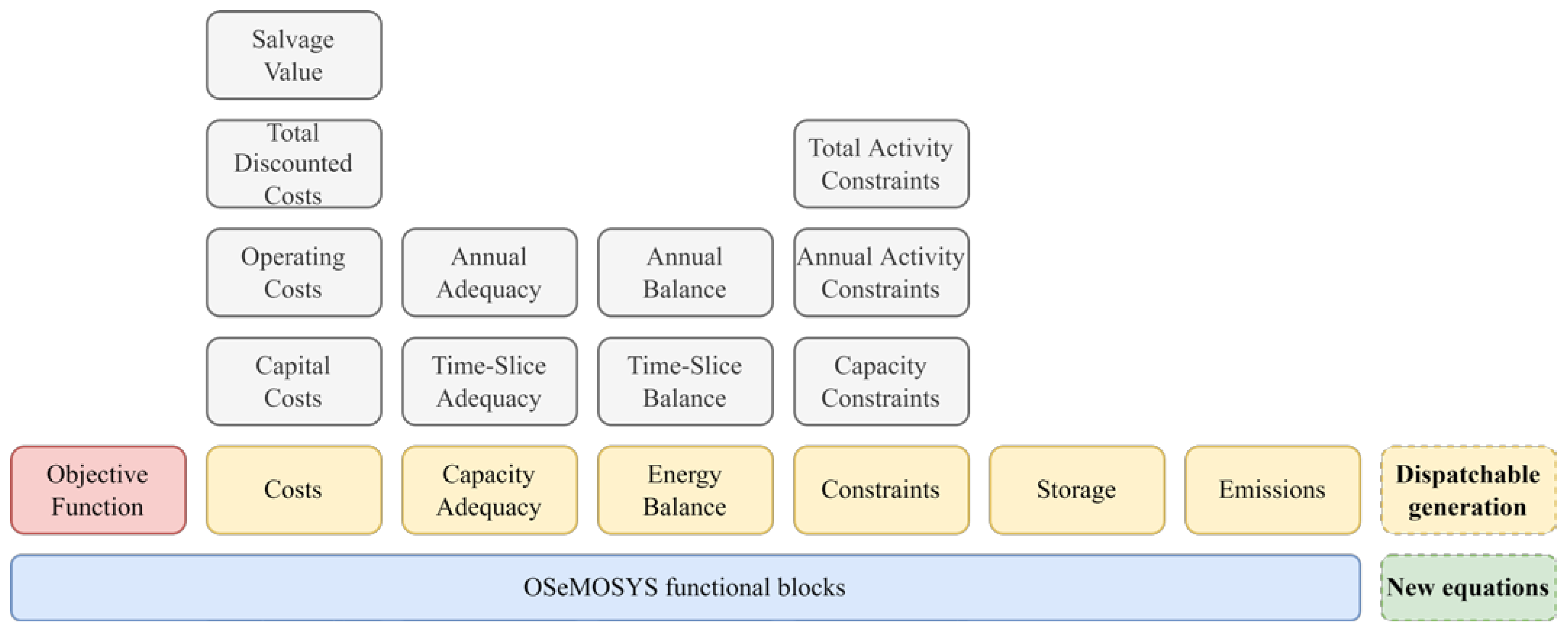
  • A new module for the OSeMOSYS framework to handle the need of dispatchable generation in energy islands;
  • A scenario analysis approach to overcome community engagement unpredictability and prioritize new RES power plants’ realization.
Therefore, the generation and combined investigation of a batch of optimal energy scenarios is introduced, based on various adoption trends of two user-scale energy technologies: distributed PV systems and EV.
The scenario analysis is developed through an energy system model of Pantelleria (Italy), which, as a medium-sized, non-interconnected island, represents a valuable and representative case study for the local energy self-sufficiency of both remote and interconnected areas. The long-run energy system evolution is studied according to the above-mentioned user-scale technology adoption trends, to identify priority energy policy measures.
The paper is structured as follows. In Section 2, the modeling framework is illustrated, the energy model and the inputs for the scenario making; in Section 3, the performed optimization results are analyzed and compared. The paper is concluded by discussing the results and the suggested contributions and outlining future research opportunities.

2. Materials and Methods

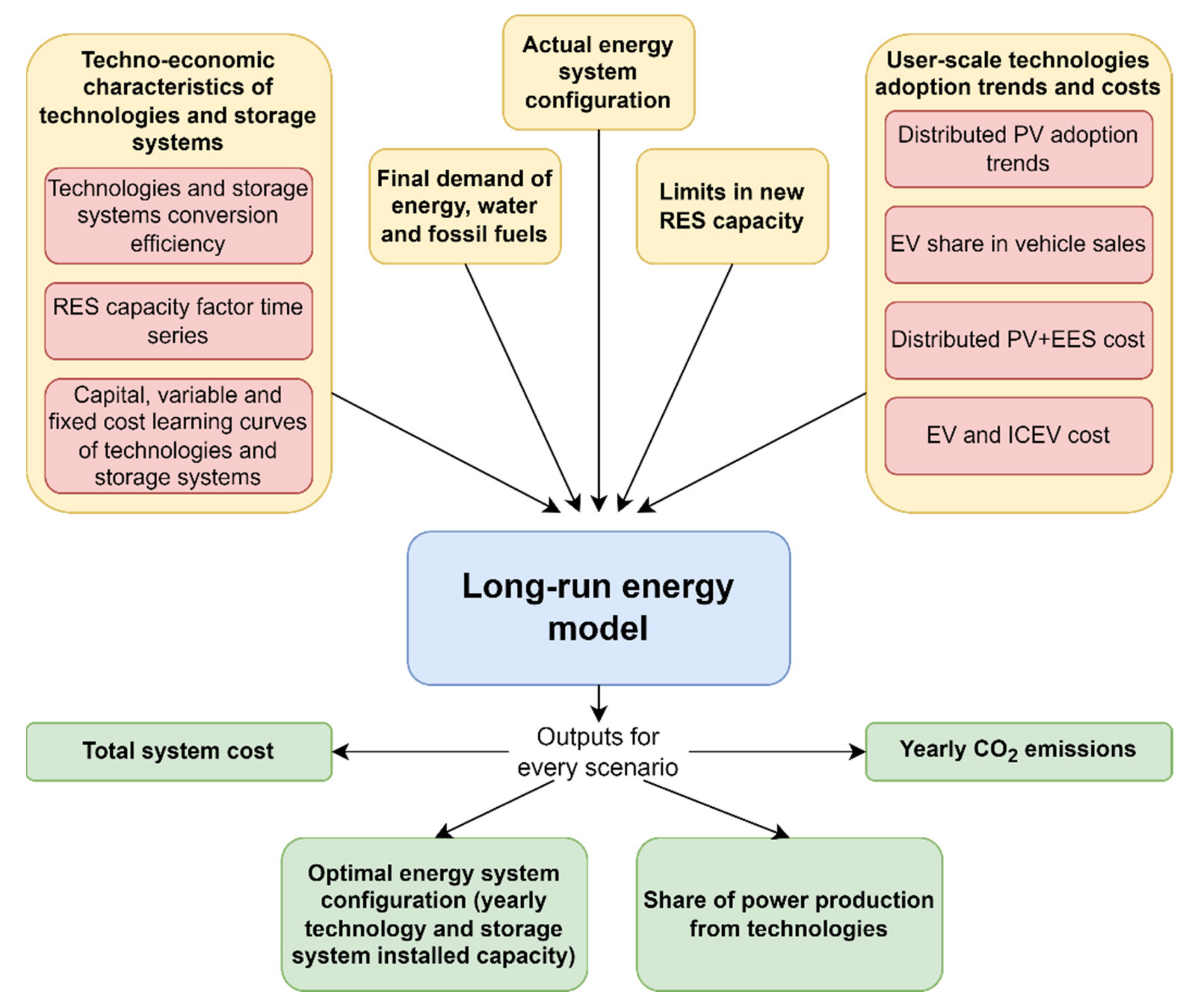
2.1. Modelling Framework

The energy model hereby presented is based on OSeMOSYS, an open-source energy modeling framework for long-term planning dating back to 2008 [39]. OSeMOSYS was selected among the bottom-up LP/MILP-based modeling tools available because of its convenient learning curve, high accessibility, and transparency; the Python version of the code was chosen because of its straightforward interoperability with libraries for datasets handling and results representation.
The energy system structure is based on two key elements: the fuels (f), i.e., energy vectors, which represent the commodities and their flows, and the technologies (t) that transform the energy vectors within the modeled system or allow their trading across the system boundaries. Every technology can have one or multiple modes of operation (m) that represent its operational configurations; for every mode of operation, a technology can have different input and output fuels. In addition to technologies, storage (s) systems enable fuel exchanges between subsequent time periods. Regarding the temporal resolution of the model, each year is divided into time slices (l) that are representative portions of the year. Time slices, as represented in Figure 1, are identified by a season, a day type (i.e., day of the season), and a daily time bracket (i.e., part of the day). All the model inputs are fixed in every time slice. The final demand for fuels can be defined on a yearly basis or on a time slice basis, depending on the model purposes and the kind of energy or energy-service demand. Concerning the spatial resolution of the model, all demands and production are related to a specific region (r), and fuel exchanges between regions may occur depending on the fixed constraints.
The modeling framework consists of the following functional blocks, as represented in Figure 2: (1) Objective function; (2) Costs; (3) Capacity Adequacy; (4) Energy Balance; (5) Constraints; (6) Storage (7) Emissions; (8) Dispatchable Generation. The first seven blocks are those of the basic OSeMOSYS implementation [23], while the last one was implemented for the application hereby presented, in view of the needs of isolated energy systems with high V-RES penetration.
The objective function to be minimized is the net present cost of the energy system to meet the given energy and energy service demands over the simulation period. In other words, it is the sum over all regions (r) and years (y) of the discounted costs of all technologies (t) and storage systems (s) [40]:
min r y t T o t a l D i s c o u n t e d C o s t B y T e c h n o l o g y r , t , y + s T o t a l D i s c o u n t e d S t o r a g e C o s t r , s , y
where TotalDiscountedCostByTechnologyr,t,y is the total discounted cost of each technology and TotalDiscountedStorageCostr,s,y is the total cost of each storage system. The key decision variables are the technology and storage installed capacity in every year and the rate of activity of technologies in every timeslice. The total installed capacity represents the sum of the newly installed capacity and of the residual capacity available from before the modeling period; the rate of activity—barring some parameters related to the technology efficiency—represents the rate at which energy is consumed or produced by the technology itself.
The cost equations are used to calculate the TotalDiscountedCostByTechnologyr,t,y. The framework makes use of three technology cost parameters: CapitalCostr,t,y (CC), that is, the capital investment cost of a technology per unit of capacity; VariableCostr,t,m,y (VC), that is, the cost of a technology per unit of activity; and the FixedCostr,t,y (FC), that is, the yearly O&M cost of a technology per unit of capacity. All costs are discounted to the first year of the modelling period. In addition, the modelling framework also considers the salvage value of technologies reaching their end-of-life after the last year of the modeling period.
Capacity adequacy equations ensure that there is enough capacity of technologies producing a certain fuel to meet its need, which is the sum of the exogenous demand and the use as input in other technologies. Equations are reported on both a time slice and yearly basis to account for both the types of fuel demands. In addition, the modeler can set a reserve margin to be provided for some fuels through the capacity of specific technologies.
Energy balance equations, on the other side, ensure that the production of fuels meets their needs in every year and timeslice.
The constraints block is related to a wide set of model inputs that allow the modeler to narrow the solution space depending on the following:
(a)
The minimum and maximum overall capacity of each technology in every year;
(b)
The minimum and maximum capacity addition of each technology in every year;
(c)
The minimum and maximum activity of each technology, both in every year and over the entire simulation period.
Additionally, the framework includes the possibility of handling some of the installed capacity variables as integer variables: In this case, the LP problem becomes an MILP problem with a general extension of the required resolution time.
The storage equations set how the storage facilities store or discharge fuels in every timeslice. The fuel demands and technology activities are the same for every timeslice, but the SOC (State-Of-Charge) of storage facilities varies along the whole year. However, as discussed in [41], extreme values of SOC can only take place in the first or last week of every season, and in the first and last occurrences of every day-type in every season. This approach allows a straightforward representation of storage systems, with a limited number of equations and, thus, a little additional computational burden.
The emission block is used to allocate pollutant emissions to the operation of a certain technology, starting from its specific emission ratio.
In this work, an additional block of equations is implemented to better investigate high V-RES penetrations within energy islands. Indeed, power grid balance and load following in energy islands must be completely addressed internally, but this is not generally studied within long-term energy models, where time-slices of several hours are the smallest analyzed time-interval. The capacity adequacy equations enable, through reserve margin, to account for the investment costs of needed dispatchable energy technologies. However, they do not allow for considering their input fuel costs, which are often preponderant in the final cost of energy from fossil fuel power plants [42]. Therefore, the dispatchable generation module sets the minimum fuel level supplied by dispatchable technologies in each time-slice. Having a minimum quantity of dispatchable generation in the energy mix is coherent with requirements from main transmission system operators, which nowadays often require a minimum share of instantaneous generation from conventional power plants for balancing grid and load services [43]. The newly implemented equations are presented as follows. The ProductionByDGTechnologyr,l,t,f,y variable is defined as:
r , l , t , f , y : P r o d u c t i o n B y D G T e c h n o l o g y r , l , t , f , y                                               = D G T a g T e c h n o l o g y F u e l r , f , t P r o d u c t i o n B y T e c h n o l o g y r , l , t , f , y
where:
r , f , t : D G T a g T e c h n o l o g y F u e l r , f , t = 1 ,     i f   t   p r o d u c e s   d i s p a t c h a b l e   f 0 ,     i f   t   d o e s n t   p r o d u c e   d i s p a t c h a b l e   f
is a binary parameter tagging the dispatchable technologies supplying every fuel, and ProductionByTechnologyr,l,t,f,y is a decision variable related to the rate of activity and representing the production of fuel by a technology in a given timeslice. The MinProductionByDGTechnologyr,l,f,y represents the minimum quantity of fuel in every timeslice to be produced by means of dispatchable generation technologies and is defined as:
r , l , f , y :   D G T i m e S l i c e L o w e r L i m i t R a t i o r , f , y , l P r o d u c t i o n r , l , f , y = M i n P r o d u c t i o n B y D G T e c h n o l o g y r , l , f , y
where Productionr,l,f,y is the sum over all the technologies of ProductionByTechnologyr,l,f,t,y, while DGTimeSliceLowerLimitRatior,f,y,l is a parameter between 0 and 1 that prescribes the portion of fuel to be produced by dispatchable technologies in every timeslice. The final constraint in Equation (5) ensures that, in every timeslice and for every fuel, the quantity of fuel produced by dispatchable technologies is higher than or equal to the minimum calculated:
r , l , f , y : t P r o d u c t i o n B y D G T e c h n o l o g y r , l , t , f , y   M i n P r o d u c t i o n B y D G T e h n o l o g y r , l , f , y
The modified code version is made available in the GitHub repository [44]. The repository also hosts a new configurator package, developed for the fill-in of multiple scenario inputs via spreadsheets.
The IBM ILOG® CPLEX® Optimization Studio software [45] was used as a solver of the MILP model.

2.2. Energy Model

The developed energy model refers to Pantelleria. The island, as a medium-sized, non-interconnected energy system, represents a valuable and representative case study for the local energy self-sufficiency of both remote and interconnected areas. Pantelleira is situated in the middle of the Strait of Sicily, as depicted in Figure 3. Because of its favorable position, it has large availability of solar, wind, and wave energy resources.

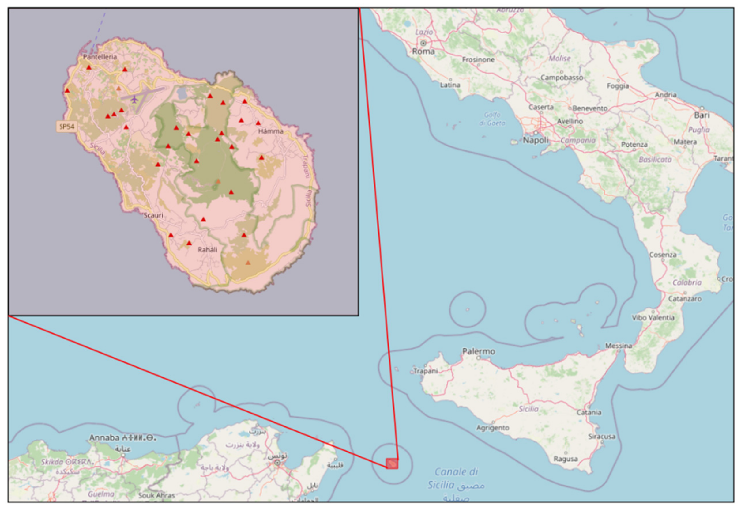
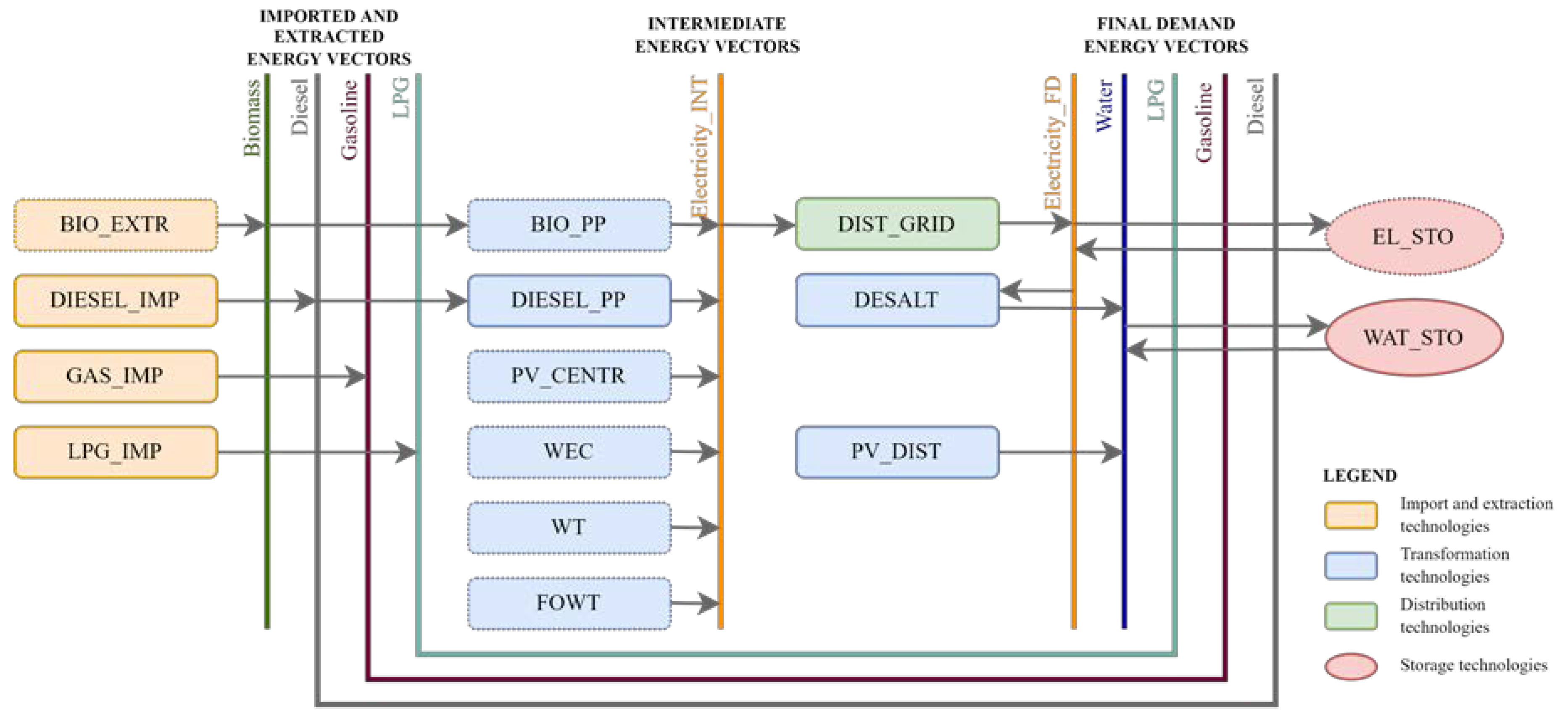
2.2.1. Reference Energy System

The reference energy system of Pantelleria is represented in Figure 4, where currently operating technologies are in solid lines, while those that were considered for the future system evolution are in dotted lines. The representation includes seven energy vectors: LPG (Liquified Petroleum Gases) and gasoline, which are imported from outside the system and consumed for kitchen applications and transportation (LPG_IMP and GAS_IMP), respectively; diesel, which is imported from outside (DIESEL_IMP) and used in diesel power plants or as a final demand for transportation; water, which is produced by electrically powered desalters; electricity, which appears in two different vectors: an intermediate vector and, after the distribution grid, as a final demand and input vector for desalters; and biomass, which is currently not exploited for the production of any of the considered energy vectors and can be internally extracted (BIO_EXTR). The transformation technologies consist of a diesel power plant (DIESEL_PP), a biomass power plant (BIO_PP), centralized (medium to large size) photovoltaic (PV) power plants (PV_CENTR), wave energy converters (WEC), onshore wind turbines (WT), floating offshore wind turbines (FOWT), and desalters (DESALT). The electricity produced by distributed PV plants is assumed to be completely self-consumed by the integration with small-scale storage systems, thus reducing the power demand to the grid. The only represented distribution technology is the power distribution grid (DIST_GRID). The storage systems are water tanks (WAT_STO), which are already used today, and electrochemical storage systems (EL_STO). The boundaries of the modeled system are the physical borders of Pantelleria Island, which is not connected to the Italian power grid but includes the surrounding sea to exploit marine RES. The energy system representation proposed here excludes the burning of biomass in home stoves for heating purposes.

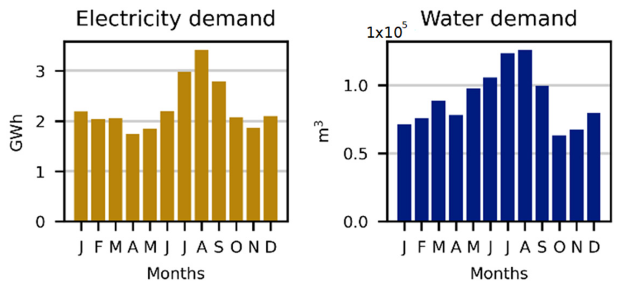
2.2.2. Commodity Demand and Supply

Water and electricity demand were specified for every time slice of the modeled period, while LPG, gasoline, and diesel demand were specified on a yearly basis. This assumption did not entail any restrictions on the energy model validity, as fossil fuels are imported from the mainland.
The actual total water supply to the municipal aqueduct amounts to ~1,070,000 m3/year. As depicted in Figure 5, the production has strong monthly variations, with a peak of over 120,000 m3/month in July/August and a trough of 62,000 m3/month in October. The water demand was communicated by the local water supplier, which manages the desalination plants, and refers to the year 2018.
The final overall electricity demand amounts to 27.3 GWh/year; as the water demand has been addressed separately, this value does not consider the energy absorbed by desalination plants (~3.7 GWh/year). As depicted in Figure 5, the demand is characterized by high monthly variability, with a trough of 1.9 GWh/month in April and a peak of 3.4 GWh/month in August. The actual total production of electricity on the island amounts to 39.0 GWh from the diesel power plant and ~0.5 GWh from distributed PV plants on households and public buildings roofs. The electricity demand profile was communicated by the local Distribution System Operator that handles the production, distribution, and sale of electricity on Pantelleria and refers to the year 2018. Overall, the monthly water and electricity demand profiles appear somehow related to each other, and they both strongly depend on the tourist numbers on the island.
Gasoline demand for transportation amounts to 19.7 GWh/year, while final diesel demand for transportation amounts to 16.3 GWh/year. LPG demand for kitchen applications amounts to 4.4 GWh/year. Data were obtained from a questionnaire compiled from the local fossil fuels retailers and are referred to the year 2018 [47].
Although all data refer to the year 2018, their validity was extended for simplicity to 2020. The evolution of the demand for energy vectors up to 2050 is described in Section 2.3.

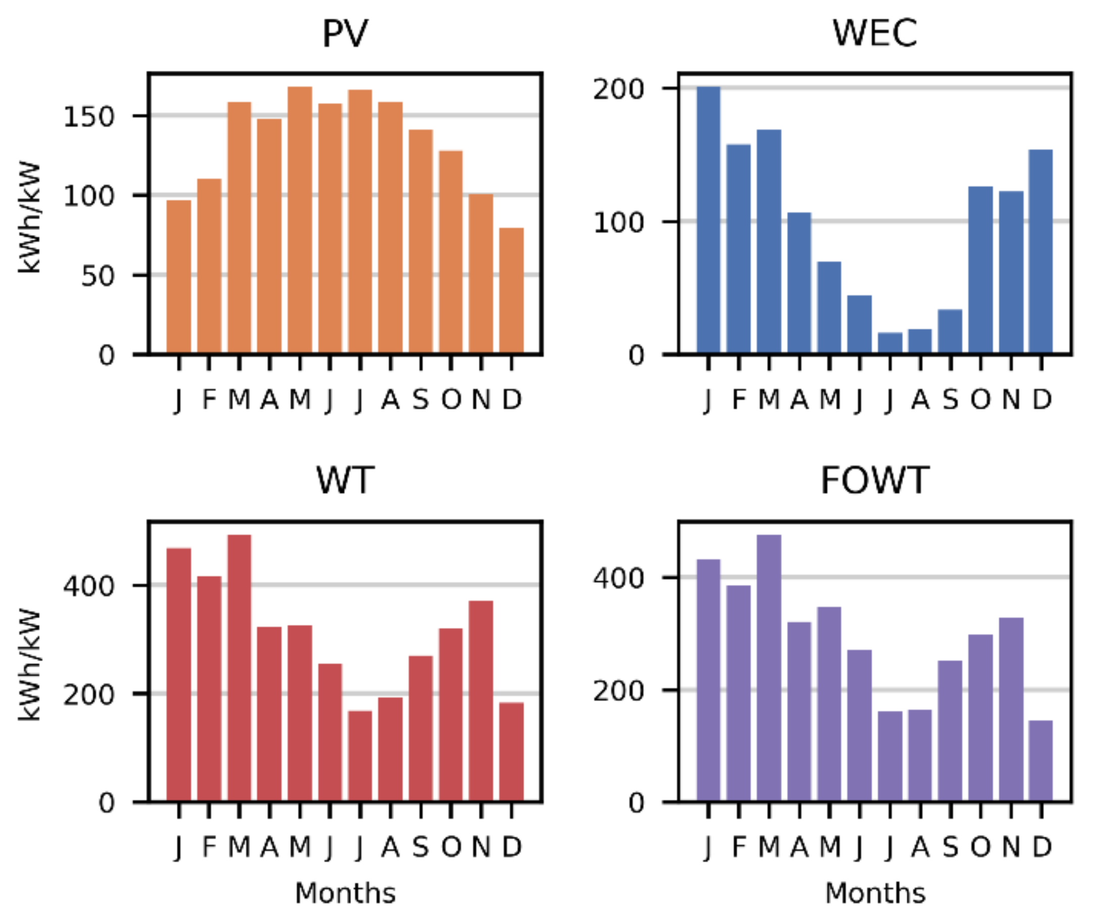
2.2.3. Technologies Specifications, Costs, and Constraints

The potential for available biomass was obtained from [48], where the maximum amount of annually extractable woody biomass on Pantelleria Island was estimated based on sustainable forest management and on the collection of agricultural mowing: It amounts to 4.2 kt/year, with an average net calorific value of 3.3 kWh/kg. The average price for its extraction was estimated at 0.151 EUR/kg [48] (VC) and was assumed as constant for the whole simulation period.
The diesel import price was estimated at 1.01 EUR/L (VC), obtained from the average net cost of diesel in Italy in 2019 [49], with a 70% surcharge deriving from Pantelleria’s insularity. The same approach was used for gasoline (VC = 0.955 EUR/L) and LPG (VC = 0.631 EUR/L).
Concerning desalination, there are currently two reverse osmosis plants on Pantelleria island: One comprises of 4 desalination modules with a production capacity of 1200 m3/day each, while the other one has a single module for 1000 m3/day. Their specific power consumption amounts to 3.5 kWh/m3. Since the realized model does not foresee the penetration of other alternative technologies, the desalination plants’ investment and management costs were excluded from the present analysis. DESALT was considered as fully programmable with water being stored in large tanks connected to the plants; the WAT_STO capacity, which was communicated by the local municipality, amounts to 20,500 m3.
The assumed BIO_PP is characterized by an overall conversion efficiency of 20%. The capital cost was estimated at 4580 EUREUR/kW (CC), while the yearly fixed costs were estimated at 40 EUR/kW/year [50]. Due to the maturity of the resource, costs were estimated to keep the same up to 2050.
The DIESEL_PP currently operating on Pantelleria Island has a capacity of 10 MW; the end of life of its generators is foreseen in 2030; their overall conversion efficiency is 39%, according to the data communicated from the company managing the power plant. The capital cost of diesel generators was estimated at 1020 EUR/kW [50] (CC), while fixed costs were neglected. Both DIESEL_PP and BIO_PP contribute to the reserve margin of Electricity_INT fuel that—as suggested in [51]—was set to 20%.
PV_CENTR power plants were assumed to consist of ground-mounted monocrystalline panels with a tilt angle of 35°. Their overall yearly productivity was estimated at 1610 kWh/kW; monthly production variability is reported in Figure 6. Hourly irradiation input data were obtained from the ERA5 database [52] for the reference year 2018. Their capital cost is 1070 EUR/kW in 2020, 520 EUR/kW in 2030, and 290 EUR/kW in 2050 [53] (CC); intermediate costs were interpolated. Fixed costs amount to 20 EUR/kW/year [50] (FC). Two constraints were set up for the centralized PV power plants: An overall maximum capacity of 6 MW for limiting the land use on the island and maximum capacity addition of 1 MW in 2021 and 2 MW in 2022 to consider the required timing to put online such plants (due to design, procurement, and permission issues).
WECs were modeled with reference to the Pendulum Wave Energy Converter (PeWEC) device [54]. The PeWEC is a floating pitching device in which wave energy conversion is carried out through one or multiple internal pendulums, each connected to a power take-off. The configuration being used here consists of two pendulum systems, with an overall rated power of 115 kW; such configuration was obtained in [55] as an optimization of techno-economic objective functions through a genetic algorithm. The overall device productivity was estimated at 1245 kWh/kW. As represented in Figure 6, the PeWEC production has a very strong intra-annual variability, with over 75% of the energy being produced in the months from October to March. The WEC hourly power production was obtained from its power matrix and the hourly sea states off Pantelleria coasts, whose parameters were taken from the ERA5 database for the reference year 2018. Capital cost was estimated at 4070 EUR/kW in 2020, contracting to 3350 EUR/kW in 2030 and 1500 EUR/kW in 2050 (CC); fixed costs amounted to 86 EUR/kW in 2020, decreasing up to 50 EUR/kW in 2050 (FC). All costs and costs projections were taken from [56], with intermediate values obtained through interpolation.
WT productivity was obtained through the power curve of the Aeolos-H 60 kW [57]. The turbine has a cut-in speed of 3.0 m/s, a rated wind speed of 9.0 m/s, and a cut-out wind speed of 25.0 m/s; it falls into the IEC III wind class [58]. The wind speed at the tower height, i.e., 22 m, was obtained through the wind profile power law and the hourly wind speeds at 10 m height from the ERA5 database [52] for the reference year 2018. The specific yearly productivity, obtained from the hourly wind speed and the turbine power curve, was estimated at 3780 kWh/kW; monthly specific production is reported in Figure 6. Their capital cost varies from 1330 EUR/kW in 2020 to 960 EUR/kW in 2030 and 735 EUR/kW in 2050 [59] (CC); their fixed cost was assumed as constant, equal to 70 EUR/kW/year [50] (FC). According to Pantelleria’s local government recommendations, the total installable onshore wind power amounts to 420 kW (7 × 60 kW wind turbines); to consider the timeline of permission, design, and procurement procedures, onshore wind turbines were considered installable from 2022 onwards.
The FOWT hourly power production profile was estimated similarly to that of onshore wind turbines by using the Vestas V80 2 MW wind turbine’s power curve at a tower height of 80 m. The turbine has a cut-in speed of 4.0 m/s, a rated wind speed of 16.0 m/s, and a cut-out wind speed of 25.0 m/s; the specific turbine model, which falls into the IEC I wind class [58], was chosen as it has been already installed on the IDEOL floating platform of the Floatgen project [60]. Floating structures were selected due to the seabed bathymetry around the island of Pantelleria, which does not allow the installation of bottom-fixed offshore wind turbines at all. The specific yearly productivity, obtained from the hourly wind speed and the turbine power curve, was estimated at 3580 kWh/kW; the value is slightly lower than for onshore wind turbines that, with their lower tower height, encounter fewer hours of wind speeds above the cut-out speed. The monthly specific production is reported in Figure 5. Due to the actual maturity level of the technology, floating offshore wind turbines were set to be installable from 2025 on. Their capacity was also treated as an integer variable, turning the model into a MILP problem. Their capital cost decreases from 3875 EUR/kW in 2020 to 2180 EUR/kW in 2030 and 1870 EUR/kW in 2050 [59] (CC); their fixed cost was assumed as constant and equal to 200 EUR/kW/year [50] (FC).
DIST_GRID is characterized by 4 independent 10.5 kV medium voltage grids starting from the diesel power plant, and the related low voltage subnets; overall, the island power network has large losses and a low level of innovation. The distribution technology was described through an efficiency of 80%. This value was obtained from the ratio between the electricity invoiced and the sum of the electricity produced from diesel power plant and distributed PV systems; all data were provided by the local Distribution System Operator. The distributed PV installed capacity (reference year: 2018) amounts to 330 kW: for consistency with the scenarios developed 2.3, and because of the averagely small size of the plants, their power production was subtracted to the overall power grid’s hourly demand, assuming a complete self-consumption by prosumers. There were no assumed costs associated with power distribution. In addition, at least 20% of the electricity production at every time slice has been set to be supplied by dispatchable technologies, in accordance with the minimum share of instantaneous conventional generation set by some European Transmission System Operators [43].
EL_STO were modeled with a 90% round-trip efficiency and an expected lifetime of 15 years. No specific depth of discharge was defined for storage systems: Results in terms of storage capacity should therefore be considered as net values to be increased according to the optimal depth of discharge of the employed technology. To enable the optimization of the discharge time at rated power, power components, and costs of energy components were entirely uncoupled, following the approach and the values suggested in [61] for Lithium-ion storage systems. This simplification enabled to explore all possible energy-to-power ratios to give information about the overall future needs in terms of energy storage systems. The input power components’ overall costs are 525 EUR/kW in 2020, 400 EUR/kW in 2025, 330 EUR/kW in 2030, and 250 EUR/kW in 2050 (CC), while the energy components global costs are 200 EUR/kWh in 2020, 155 EUR/kWh in 2025, 130 EUR/kWh in 2030, and 95 EUR/kWh in 2050 (CCS) [61]. All intermediate values have been interpolated.
The capital and fixed costs of technologies and the capital costs of storage systems at the reference years 2020, 2035, and 2050 are summarized in Table 1, while the variable costs of fuels supply are summarized in Table 2.
It is worth mentioning that the current regional regulatory landscape does not allow the exploitation of wind power on Pantelleria and limits the installation of ground-mounted PV to the urban area. However, the local administration, supported by the authors, has started revising the regulations that are considered incompatible with an ambitious decarbonization process [47]. The main guidelines under discussion have been used in this work to define the capacity constraints.

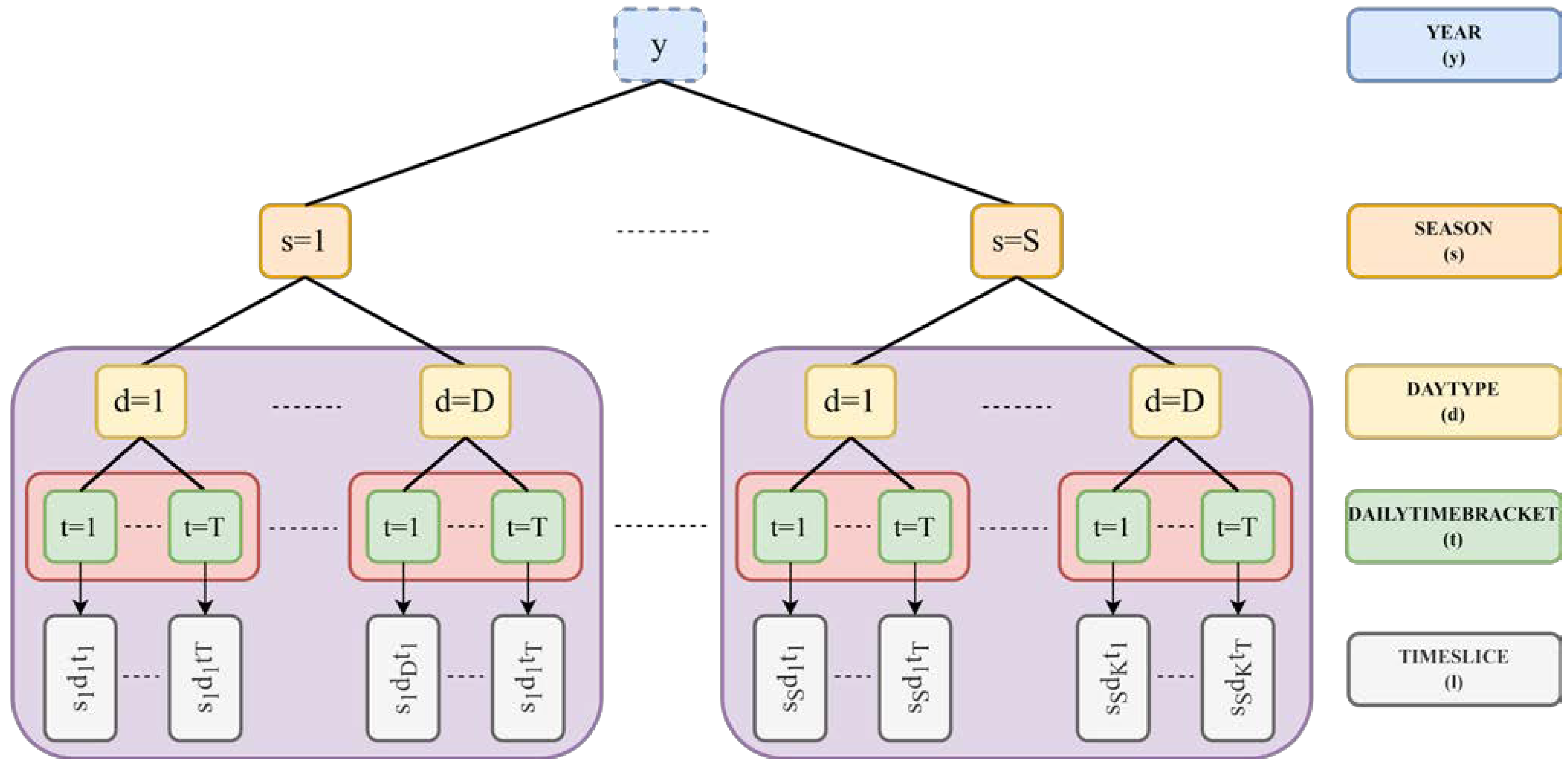
2.2.4. Time Representation

The same time representation was used for all the years in the simulation period. Every year was firstly divided into 5 seasons. Each season was then further broken down into weekdays and weekends to contemplate energy consumption differences within the week. Finally, to consider intra-day variability of electricity consumption and solar radiation, each day was divided into 5 timeslices. A total number of 50 time slices per year was therefore used. Details about the employed seasons, day types, and daily time brackets are reported in Table 3. All the needed time series, i.e., those related to power consumption, water consumption, and power production from RES were summed in the corresponding timeslices.

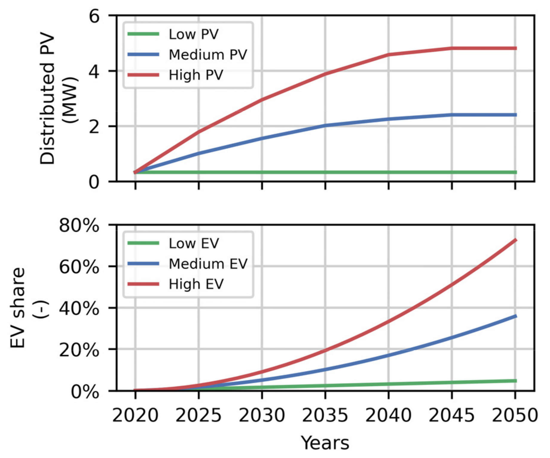
2.3. Scenario Settings
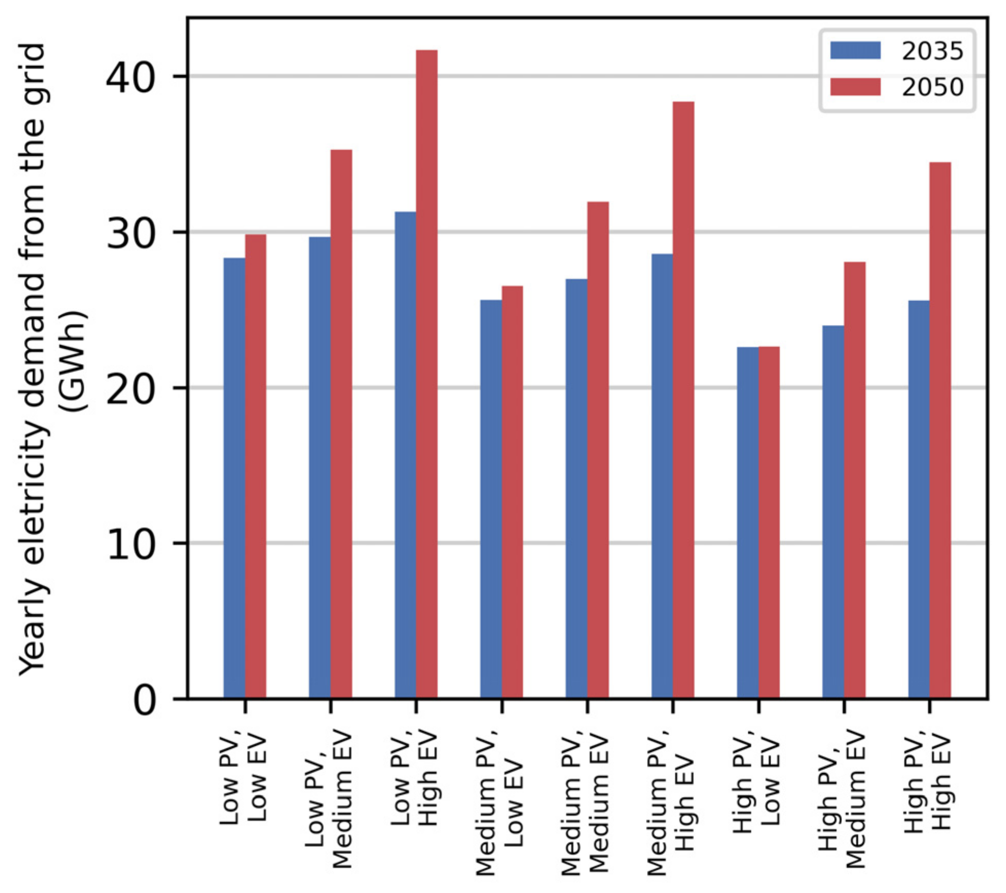
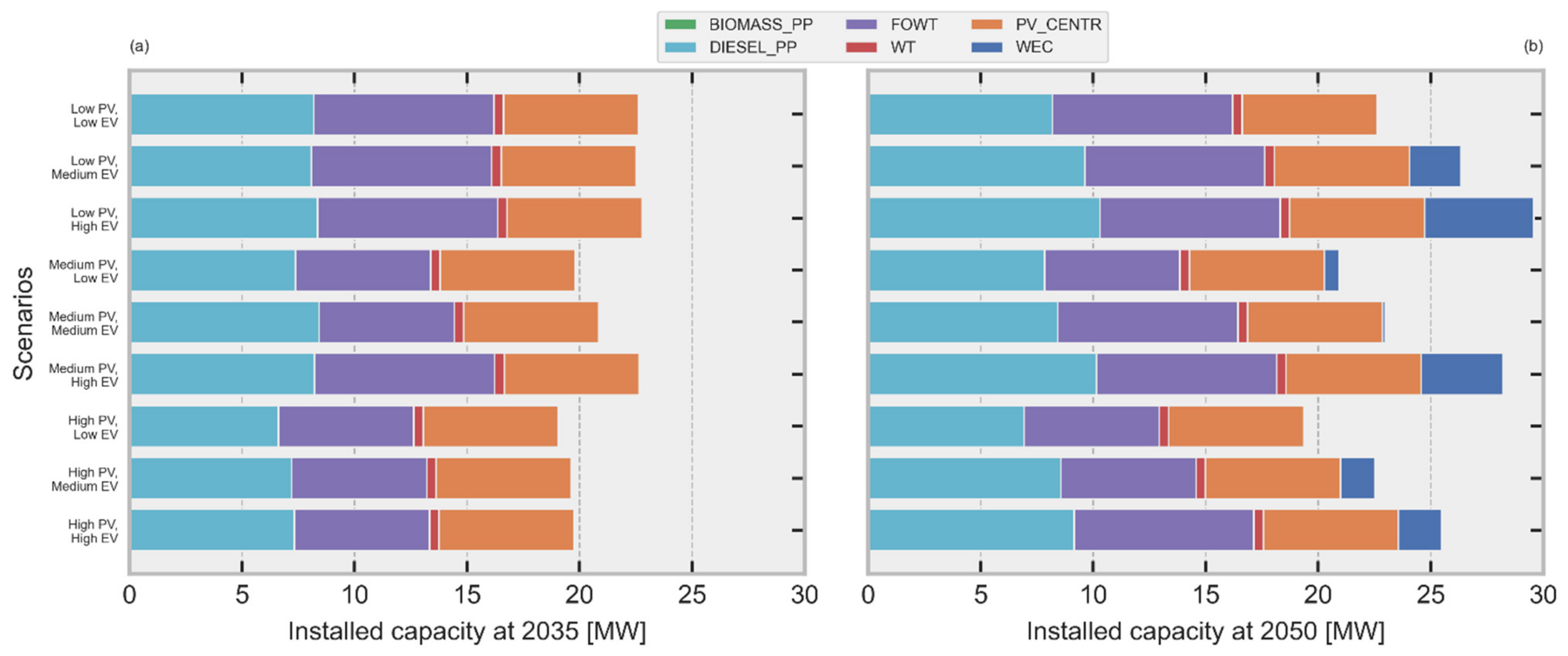
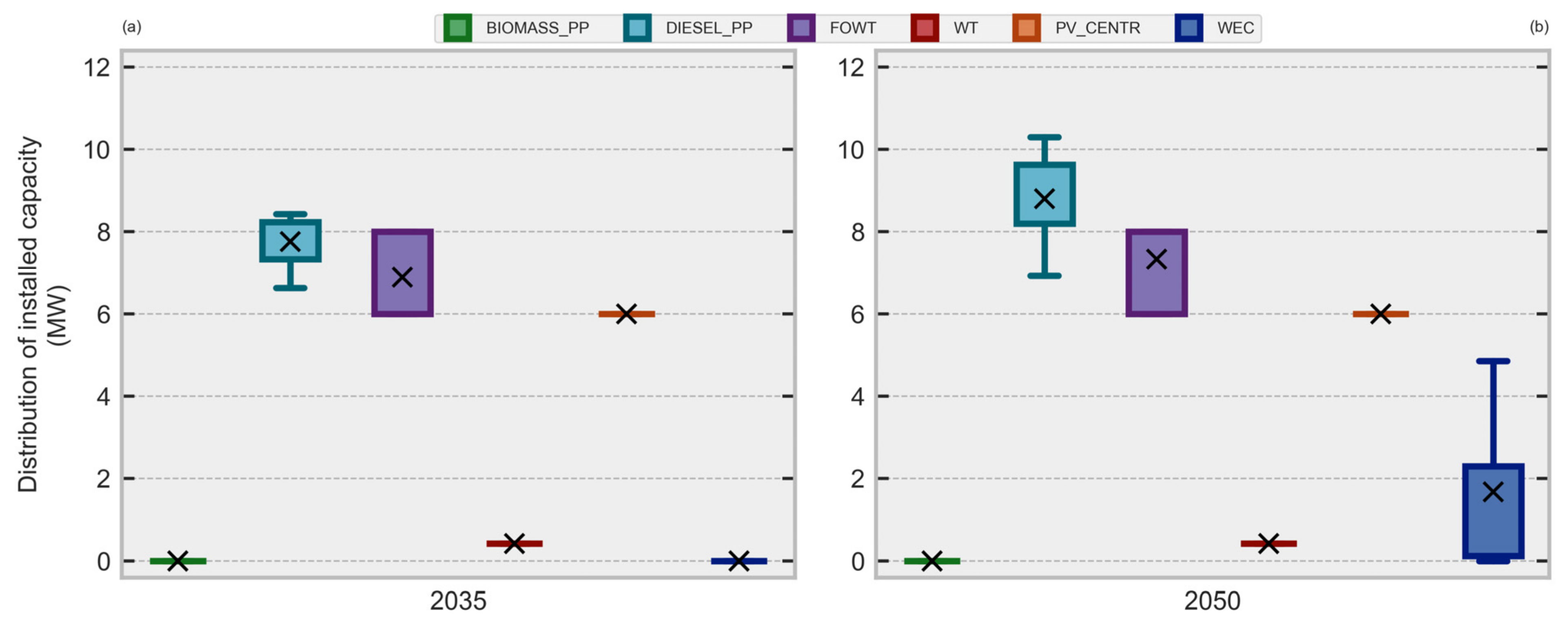
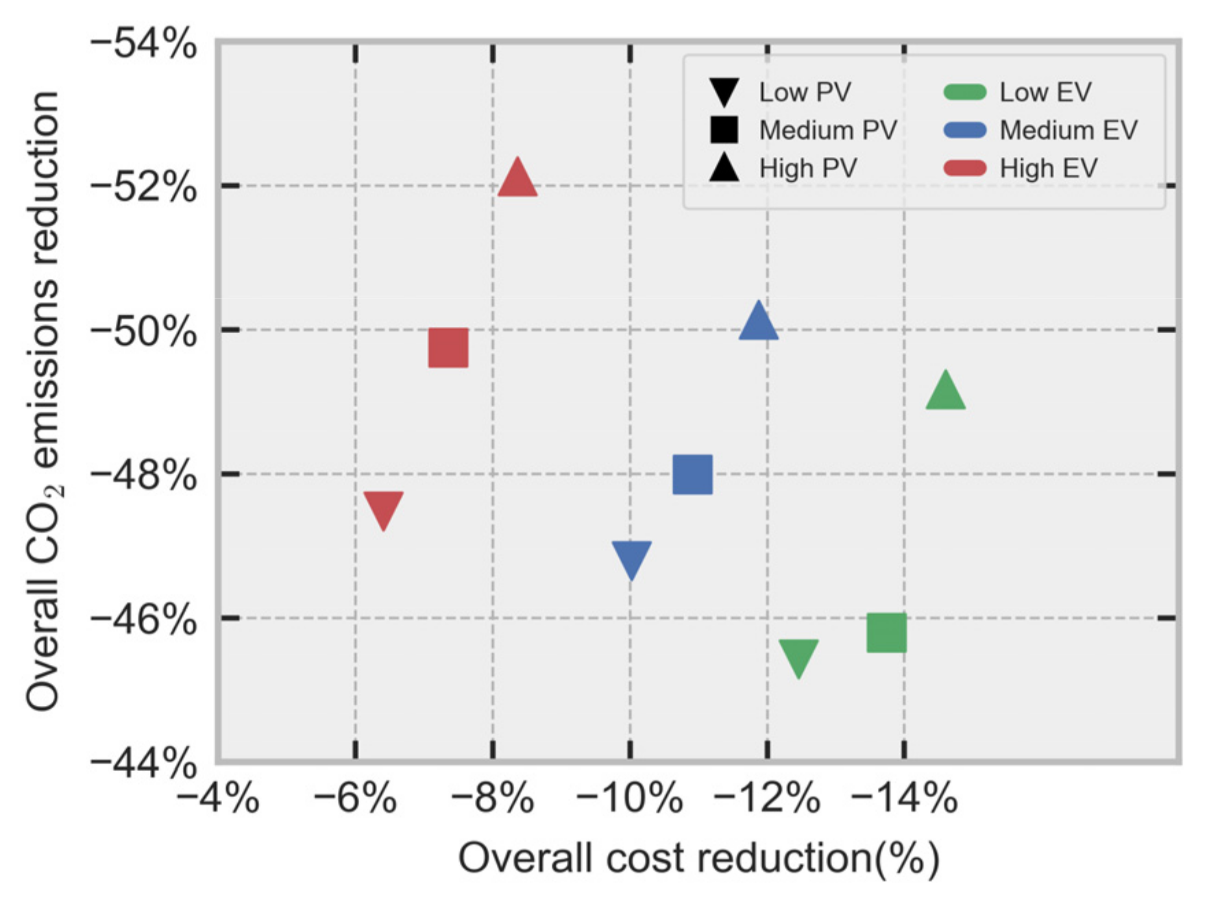
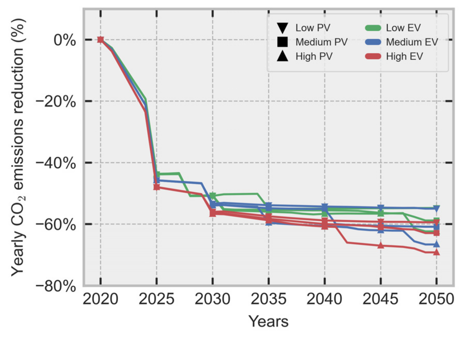
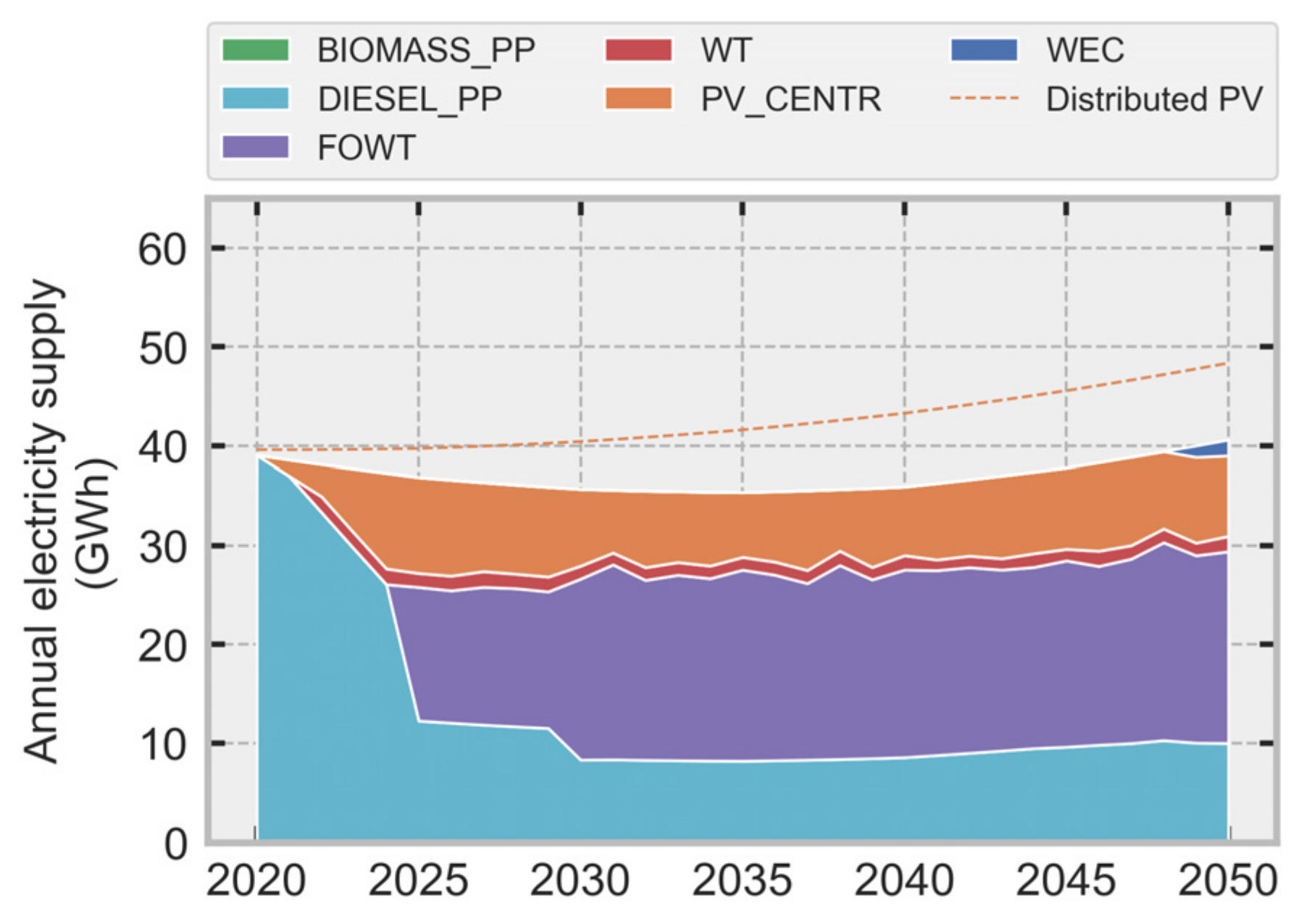
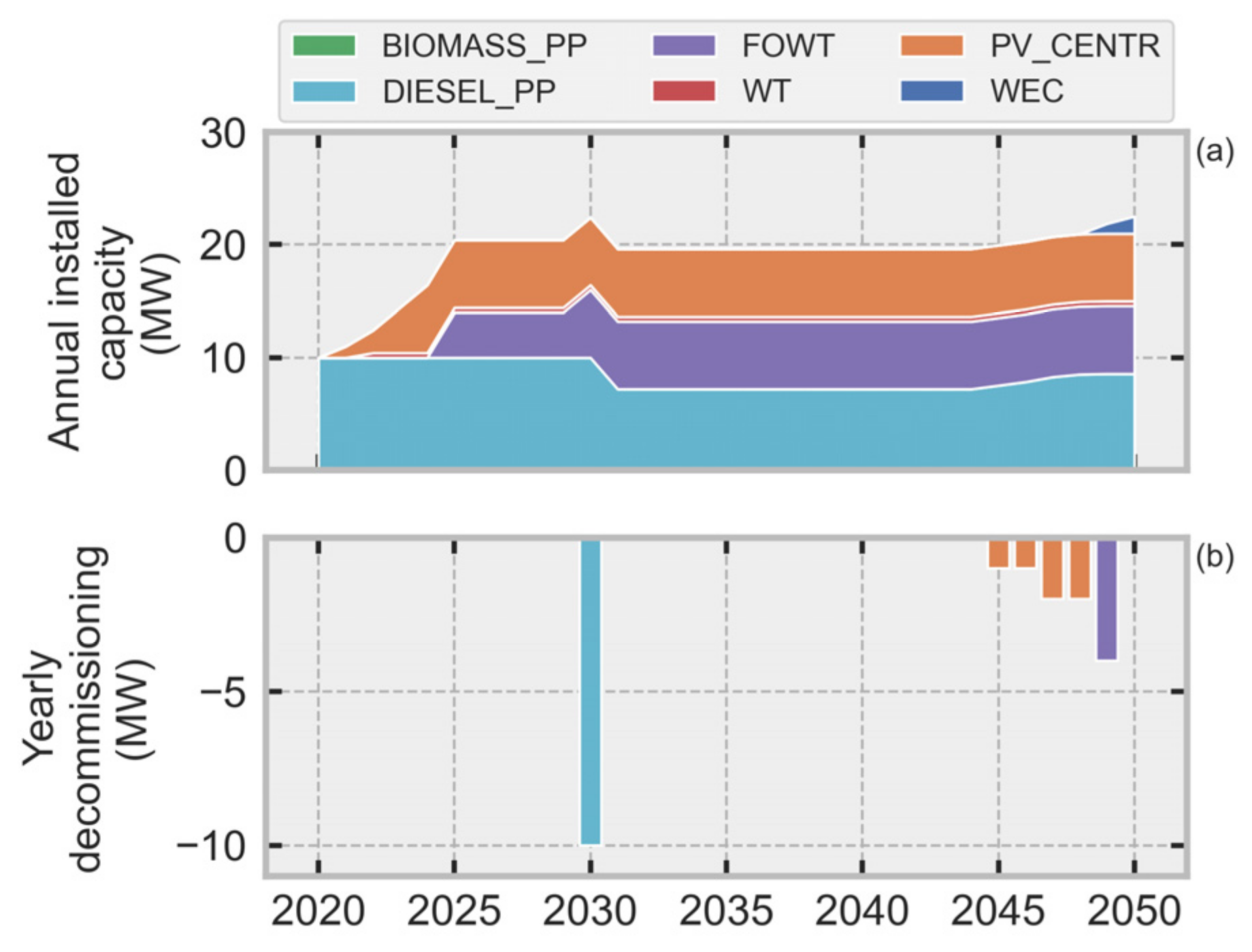
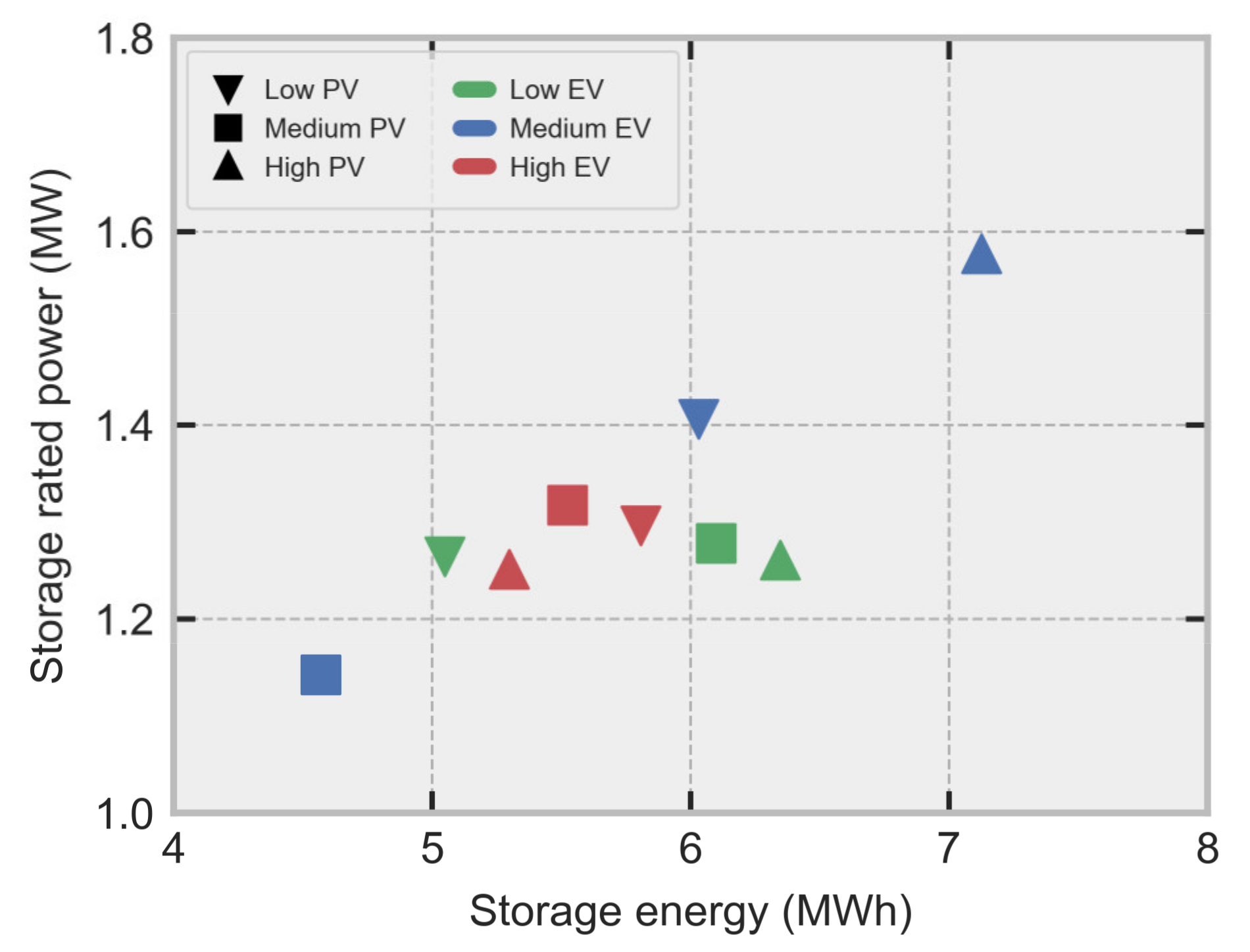
Future energy scenarios were explored in terms of the evolution of two macroscopic variables related to citizens direct engagement in the energy transition process and, specifically, to the adoption of consumer’s technologies: the diffusion of roof-mounted distributed PV with related storage systems and the diffusion of Electric Vehicles (EV) on the island. These two factors are expected to have a substantial impact on the local energy system evolution, especially in terms of the energy provision cost and its related emissions. Additionally, both the diffusion of distributed PV and EV are features that can be powerfully conveyed on the island by public energy policies, namely, through the permission for installing PV panels on buildings roofs (which is mostly not allowed by today on Pantelleria) and the incentives for replacing Internal Combustion Engine Vehicles (ICEV) with EV. Three different evolutions were foreseen for each of the two variables, leading to nine policy scenarios in total.
The settings for PV systems diffusion were developed based on different expected evolutions of the per-capita distributed PV rooftop installed capacity. The Low PV scenarios do not envisage any increase in the actual distributed PV systems penetration, which amounts to approx. 0.04 kW/person of PV. The Medium PV scenarios consider an increase up to 0.30 kW/person, achieved especially from now until 2035, while the High PV scenarios forecasts up to 0.60 kW/person, ensuring the 65% self-sufficiency of the residential sector. Table 4 presents the details of the parameter evolutions at the years 2020, 2035, and 2050. Figure 7 (top) represents the resulting evolution of the overall distributed PV capacity for the sets of scenarios. All distributed PV systems have been assumed to be equipped with an Electrical Energy Storage (EES) system for the maximization of self-consumption. The indicative sizing of the system was obtained from [62], where a 4-kW PV system for domestic applications was equipped with a 6.4–3.3 kW EES, ensuring an almost full self-consumption of the energy produced. The needed storage capacity was thus estimated at 1.6 kWhEES/kWPV. The distributed PV system costs were estimated at 2140 EUR/kWPV in 2020, with a lifetime of 26 years, while the EES costs were estimated at 1350 EUR/kWPV in 2020, with a lifetime of 13 years [62]. The evolution of costs, presented in Table 5, was obtained using the same cost reduction rate of the centralized PV and electrochemical storage technologies.
The settings for EV diffusion were developed based on the policy scenarios defined in the Global EV Outlook 2020 by IEA [63], which forecasts the share of EV sales in 2025 and 2030 depending on the environmental sustainability level of global energy policies. The Low EV scenarios entail a fixed share of EV sales, equal to the share in 2019 (2.8%), for the whole studied period. The Medium EV scenarios follow the IEA’s Stated Policies Scenario, which forecasts an EV sales share of 9.4% in 2025 and 15.7% in 2030. The High EV scenarios, finally, follow the IEA’s Sustainable Development Scenario, with an EV sales share of 18.0% in 2025 and 31.5% in 2030. Trends have been linearly extrapolated up to 2050, with a final EV sales share of 40.9% for the Medium EV scenarios and 85.5% for the High EV scenarios. The yearly vehicle stock renewal rate has been calculated as the mean value of the last 20 years for Italy, which amounts to 5.54%, while the total amount of ICEV currently circulating in Pantelleria is 9560 [64]; both these values have been assumed as constant along the whole model period. Because of the rural environment of Pantelleria, the vehicle stock has been assumed to consist of 50% of passenger cars and 50% of SUVs/pick-ups/light trucks. Also, ICEV have been assumed to be equally divided between gasoline and diesel vehicles. Figure 7 (bottom) represents the resulting evolution of the EV share on the total vehicle stock for the sets of scenarios. The resulting average cost for the purchase of ICEV was estimated at 26,240 EUR/vehicle, which is considered constant along the whole simulation period. The average cost of EV in 2020 has been estimated at 48,450 EUR/vehicle, decreasing to 43,610 EUR/vehicle in 2035 and to 40,170 EUR/vehicle in 2050. Costs of vehicles and their future evolution trends were obtained from [65].
The costs of vehicles and PV systems purchased for the simulation period were actualized to the year 2020 and added to the total energy system cost; moreover, the salvage value of technologies not reaching end-of-life by the end of the modelling period was considered. The overall effect of the parameters’ evolution resulted in a change of the final energy demands for the different scenarios. The increase in distributed PV systems capacity leaded to the progressive decrease of the electricity demand in the model inputs, under the hypothesis that all the produced electricity is self-consumed in households. The diffusion of EV leads to a decrease in diesel and gasoline demands and to an increase in electricity consumption; those two variations are correlated by the values of the overall efficiency of ICEV (35%) and EV (85%). In addition, all scenarios include the complete electrification by 2050 of the electric stoves that LPG almost entirely covers today.
Thus, the model parameters that vary between the scenarios are the electricity annual demand and the annual demand of diesel, gasoline, and LPG. The annual electricity demands from the power grid in 2035 and 2050 for the different scenarios are presented in Figure 8: It can be observed how differences in the energy demand in 2035 are less pronounced than in 2050. The peak demand (41.6 GWh in 2050) is reached by the Low PV, High EVs scenario, while the lowest demand is that of High PV, Low EVs. Overall, the impact of EV share on the final demand from the power grid is higher than that of distributed PV diffusion.
For each scenario, the resolution algorithm optimized the overall cost of the global energy supply from 2020 to 2050 by setting, in accordance with the fixed constraints, the power plants rated power, the electrochemical storage rated power and discharge time, and the energy that each of these systems fed into the grid in every timeslice. Results were compared in terms of economic and environmental benefits with respect to the Business As Usual (BAU) scenario, where the same energy consumption and energy mix of 2020 was upheld up to 2050.
A summary graphical description of the applied methodology with a focus on the model inputs and outputs is depicted in Figure 9.

3. Results

A first overview of the results is depicted in Figure 10, which represents the installed capacity by technology for every scenario in 2035 (a) and 2050 (b). In 2035, the total installed capacity is quite similar among scenarios, with total values in the range of 18 to 23 MW. Especially, all the Low PV scenarios and Medium PV, High EV, characterized by the highest power demand from the grid, require higher installed capacity. The key differences among scenarios are mostly in terms of DIESEL_PP and FOWT capacity. In 2050, the differences are more pronounced, with overall capacity values in the range of 18 to 30 MW. The production fleet does not significantly change from 2035 to 2050 for Low PV, Low EV and High PV, Low EV, while it meets significant evolutions in the other scenarios, also with the inclusion of variable WEC capacity. Especially, Low PV, High EV is the scenario requiring the highest overall installed capacity (over 29 MW), followed by the Medium PV, High EV scenario (approx. 28 MW).
The boxplot in Figure 11 represents the most frequent ranges of installed capacity over the set of scenarios in 2035 and 2050. The chart makes it possible to identify the minimum needed installed capacity of each technology independently of the possible trend of adoption of the two analyzed consumer’s technologies, as well as its distribution among scenarios. The results show strong consistency among scenarios, with PV_CENTR and WT reaching their maximum values already in 2035, 6 MW and 420 kW, respectively, and BIOMASS_PP—characterized by high fuel costs—not resulting in any scenario at any year. The capacity of offshore wind turbines is in the range 6–8 MW both in 2035 and 2050, with a slightly higher mean value in 2050 than 2035. DIESEL_PP range is 6.6–8.4 MW in 2035, with a mean value of almost 8 MW. The range is even higher in 2050, with a minimum value of 6.9 MW, a maximum value of 10.3 MW, and a mean value around 9 MW. The WEC technology, despite not being included in any scenario in 2035, is characterized by a large installation range in 2050, between 0 MW and 4.8 MW, with a third quartile of over 2 MW. It is worth mentioning that WECs are also included in the technology mix when FOWT saturation is not reached, as in Medium PV, Low EV and High PV, Medium EV.
The scatter plot in Figure 12 presents the scenario outcomes in terms of cost reduction and direct CO2 emissions reduction with respect to the BAU; both variables are considered on the whole model period. The potential energy system cost reduction is in the range of 6–15%, and the CO2 emissions reduction is between 45% and 52%. The most significant cost reduction is obtained for High PV, Low EV, followed by Medium PV, Low EV and by Low PV, Low EV. All the Medium EV and High EV scenarios present higher energy system costs, thus indicating that the higher investment cost of EV compared to ICEV is not balanced by the overcosts for fuel supply on the island. Nevertheless, High PV, High EV is the scenario performing the best in terms of overall CO2 emissions, with a reduction compared to BAU of over 52%. All High EV scenarios perform better in terms of CO2 emissions when compared to the corresponding ones in terms of distributed PV diffusion. Overall, High PV scenarios can be considered the best ones, as they always perform better than the corresponding scenarios for EV diffusion on both the chosen evaluation parameters.
A further yardstick is the evolution of the yearly CO2 emissions for the set of scenarios. Figure 13 illustrates the yearly CO2 emissions compared to the BAU scenario. Strongly ambitious targets, around 70% carbon emissions reduction, are reached by 2050 for High PV, High EV and High PV, Medium EV, while most scenarios reach ~60% reduction. In addition, it is observable how all scenarios reach 45% carbon emissions reduction by 2025, highlighting the low cost-effectiveness of the actual electricity mix. Nevertheless, after 2025, the increase in RES penetration is slower, also due to the saturation of the identified technical potential of cheaper sources, namely, PV_CENTR and WT; further V-RES penetration is then smoother, and it depends on the progressive reduction of their costs.
A more detailed breakdown of the results in terms of evolution of the technology and the energy mix is given below. The scenario High PV, Medium EV, which demonstrated a good trade-off between environmental and economic sustainability, was selected as a representative example. The stack plot of Figure 14 displays the evolution of the energy mix in the simulation period. The total electricity production increases from ~40 GWh in 2020 to ~48 GWh in 2050. Overall, electricity production from centralized power technologies decreases from 2020 to 2035, thanks to the distributed generation of rooftop PVs. Nevertheless, from 2035 onwards, the demand for electricity progressively increases because of EV diffusion. It is also noticeable how electricity production from DIESEL_PP strongly decreases in the first five years, has a further fall in 2030, and then slightly increases because of the set constraints in terms of the minimum share of electricity produced from dispatchable technologies; it reaches 10.0 GWh in 2050. In 2050, the largest portion of production from V-RES is that of FOWT, with 19.4 GWh, followed by PV_CENTR, with 8.1 GWh. WT and WEC both generate 1.6 GWh in 2050; however, while WT reaches this value already in 2022, WEC is included in the energy mix in the very last model year.
The charts in Figure 15 represent (a) the annual installed capacity and (b) the yearly capacity decommissioning by technology. The capacity of DIESEL_PP remains the same up to 2030, when the existing plant reaches its end-of-life and must be replaced; its capacity then slightly increases in the last five years. FOWT reaches 6 MW in 2025, increasing to 8 MW from 2030 on. The available PV_CENTR capacity becomes saturated already in 2025, while 420 kW of WT are installed already in 2022. In 2029, finally, 1.5 MW of WEC are added in the technology mix. All RES technologies are fully replaced when they reach end-of-life. The energy mix varies with a similar trend, except for what concerns DIESEL_PP: The plant reaches its end-of-life in 2030, but strongly decreases its operation already in the first decade. The diffusion of V-RES and the consequent decreases in power production from dispatchable technologies do not correspond to a significant reduction in the capacity of dispatchable technologies but mainly involves a reduction in their utilization factor. The energy mix in 2050 is made up as follows: 40.1% FOWT; 20.7% DIESEL_PP; 18.7% Distributed PV; 18.6% PV_CENTR; 3.3% WEC; 3.2% WT. The penetration of DIESEL_PP on a yearly basis in 2050 is then slightly higher than the minimum levels of dispatchable generation in every time-slice.
For all policy scenarios, the performed optimizations resulted in a specific capacity of energy-intensive storage systems. As shown in Figure 16, optimal storage systems in 2050 have quite different requirements in terms of energy sizing, in the range of 4.6–7.1 GWh, while they present small differences in terms of rated power, in the range of 1.1 to 1.6 MW. The three scenarios requiring the highest storage energy, namely, Medium PV, Low EV; High PV, Low EV; and High PV, Medium EV, are those characterized by the lowest electricity demands from the grid, and thus by the lowest demand peaks, as well as by the lowest minimum dispatchable generation levels. In such scenarios, the lower FOWT installed capacity seems to justify larger storage energy. The obtained storage characteristics indicate that they could mainly be used in load-levelling applications, as well as for the mitigation of V-RES, partially reducing their curtailment. In addition, it should be noted that the storage capacity of EES coupled with distributed PV amounts to 3.8 MWh in Medium PV scenarios and to 7.7 MWh in High PV scenarios in 2050.

4. Discussion

This paper’s main contribution is to tackle the unpredictability of citizens’ commitment when planning the decarbonization of local energy systems. The results show that different evolutions of distributed PV adoption and EV diffusion may highly impact the optimal configuration of energy systems, supporting the need for prioritizing interventions and RES installations according to their robustness with respect to future uncertainties. Furthermore, the proposed scenario analysis quantifies the positive and negative impacts related to the spread of user-scale energy technologies, highlighting the most desirable evolutions in terms of economic and environmental sustainability. In comparison to other approaches for studying uncertainties in long-term energy modelling [34,36], which make use of real-world datasets or reference distributions to discover key variables and highlight optimal strategies, the implemented procedure is more specific. Nevertheless, it does not require large datasets or input distributions and focuses on the prioritization of energy and policy actions, making it realistically applicable at the local scale and by a wider audience.
For the case study of Pantelleria Island, in which a technical potential was set for all RES power plants and no minimum environmental targets were defined, it is found that High PV diffusion can lead to the strongest reduction in yearly CO2 emissions, up to −70% with respect to BAU; other scenarios do not perform better than −60%. In addition, High PV scenarios always bring lower energy supply costs than the corresponding Medium PV and Low PV ones. Distributed PV + EES systems, characterized by higher costs than PV_CENTR, are more cost-effective of less mature power production technologies, as FOWT and WEC. Moreover, PV_CENTR potential is always fully exploited independently of the adopted distributed rooftop PV diffusion trend; this result shows that peak production in the central hours of the day is acceptable, even at the expense of high investments for storage systems or RES curtailment. Overall, the outcomes demonstrate that High PV scenarios can lead to a 90–100% increase in the overall share of PV systems when compared to Low PV ones. This expected increase is not very different from the outcomes by Gernaat et al. [37], which obtained a 80% increment in the total share of PV when including distributed rooftop PVs in a global energy scenario. The observed difference may be explained as follows: Firstly, the PV_CENTR potential of Pantelleria is limited because of numerous landscape and environmental constraints; secondly, distributed PV systems were combined with EES, assuming no curtailment for rooftop PV, thus the higher productivity than utility-scale PV in an energy system with high V-RES penetration.
Concerning EV penetration, it was evaluated that High EV scenarios lead to an overall electricity consumption increase of 40% with respect to scenarios with only ICEV in 2050. Compared to Krause et al. [38], who estimated an increase of 30% in EU electricity consumption for a road transportation high electrification scenario by 2050, a higher relative rise was obtained; such difference can be justified by the lower per capita yearly electricity consumption in Pantelleria compared to the European average (3.4 MWh/person vs. 5.3 MWh/person [66]), partly offset by a lower per capita yearly fuel consumption for road transportation (5.4 MWh/person vs. 7.0 MWh/person [66]). Nevertheless, it was also noted that higher EV penetrations always entail higher energy system costs in Pantelleria, with an average 10% over the cost of High EV scenarios with respect to Low EV ones. This result is mainly related to the larger investment cost of EV with respect to ICEV that, despite a progressive contraction, was estimated to be +53% in 2050.
With respect to previous research studying the long-term impacts of distributed PV [37] and EV adoption [38], this paper focuses on a local scale, obtaining results that are less applicable to a general scale. However, a methodology that studies the combined diffusion of the two user-scale technologies is proposed, identifying distributed PV + EES systems and, therefore, the self-sufficiency of households, a major factor for the achievement of high decarbonization targets under economic sustainability. A high penetration of EV, which entails a significant increase in mobility costs, must be adequately accompanied by investments in renewables to ensure a consistent reduction in overall carbon emissions. Above all, the impacts of community engagement uncertainties on the optimal future energy mix are analyzed, concluding that established technologies, namely, PV_CENTR and WT, are by far the most competitive and their potential—which was set for the analyzed rural energy system—is always saturated. Key differences between scenarios are in the capacity of novel power technologies, i.e., FOWT and WEC, and of fossil fuel power plants (DIESEL_PP). The maximum observed differences are in the order of 25% for FOWT and 45% for DIESEL_PP; moreover, WEC is the technology with the largest uncertainty, in the range of 0 to 4.9 MW. Lastly, the optimal sizing of STO_ELC also shows great variations between scenarios, with a maximum relative difference of 55%.
The present work also suggests some interesting outcomes for the energy transition of islands and isolated areas. An electricity mix largely based on renewables can be economically advantageous for those energy systems with no connection to national power grids and with overcosts for fossil fuel supply. Compared to the study of Mauritius energy system by Timmons et al. [28], a similar share of fossil fuel power generation is obtained in the least cost scenario, around 21 to 22%. In addition, in the Mauritius case study—for which technology costs were kept constant along all model period—researchers have identified an additional 11% share from locally produced sugarcane bagasse and no electrochemical storage systems were included. In the present case study, where technology learning curves were used, BIO_PP never resulted in being competitive, while energy-intensive utility-scale electrochemical storage systems were included in all scenarios.
From a critical analysis of the results, certain indication emerges for future developments of the implemented approach. First of all, the diffusion of EV leads to a significant increase in electricity demand, and it is worthwhile developing appropriate methodologies for including the deriving potential demand flexibility in long-term LP- and MILP-based models: This could lead to a reduction in the expected V-RES curtailment and to an overall lower required capacity of power generation technologies. Secondly, developed scenarios rely on technologies that are not yet fully mature. The cost evolution of the studied technologies, both user-scale and utility-scale ones, can be a major factor in identifying the optimal future energy mix: It would therefore be interesting to evaluate the solidity of results with different learning curve projections. Thirdly, the obtained results may be affected by the adopted time-representation. Notwithstanding the large number of timeslices that was used, long-term optimization models underestimate generation and load peaks and are not capable of considering the future need for power-intensive storage systems. This weakness could be partially overcome through the introduction of pre-processing algorithms for the optimal choice of timeslices, which could lead to tighter granularity around generation and load peaks.

5. Conclusions

The level of citizens’ commitment in the energy transition may lead to different trends in the adoption of user-scale technologies. Primary importance is held by distributed PV systems and EV, whose diffusion is expected to strongly affect future energy demand from the grid. However, little effort has been devoted to studying the long-term impact of these factors on the evolution of energy systems towards decarbonization. Above all, such uncertainties can affect the optimal power electricity mix of those local systems with no or limited connection to national grids, as well as of areas aiming at energy self-sufficiency. Therefore, this study presents a novel scenario analysis approach based on the combined study of distributed PV and EV diffusion up to 2050. The suggested technique provides guidance on the prioritization of power plants to be realized and energy policies to be implemented, with an eye on the potential contribution of technologies under development. A revised OSeMOSYS framework is used to model the energy system of Pantelleria as a non-interconnected island, which represents a valuable case study for the implementation of policies towards local energy self-sufficiency.
In conclusion, it can be stated that the diffusion of distributed PV + EES systems represents a key factor for the achievement of high decarbonization targets and that—based on technology learning curves—it also represents a cost-effective solution. For the implemented case study, indeed, High PV scenarios always ensure CO2 emission reductions of at least 49% and overall cost reductions of at least 8% compared to BAU. The diffusion of EV, on the contrary, requires considerable capital costs, as well as larger overall installed capacity. Consolidated power production technologies—namely, PV and WT—are installed from the very first years. Furthermore, novel technologies—FOWT and WEC—are also progressively installed; their optimal capacity, however, features large differences depending on the foreseen evolution of user-scale technology adoption trends. The optimal installed capacity of FOWT varies in the range of 6–8 MW in 2050, while that of WEC varies in the range of 0 to 5 MW.
It is worth mentioning that the proposed technique, although it does not make use of large datasets on user-scale technologies, requires an accurate description of the local energy system under study. Furthermore, the results in terms of the optimal energy system configuration highly depend on the available technical potentials identified for the energy system under study; this aspect must be carefully addressed with decision makers considering environmental and landscape constraints, as well as local community needs. In addition, the implementation of MILP-based long-run energy models requires the use of time slices to limit the computational burden. The resulting averaging of input time series (power load and V-RES production profiles) leads to a reduction in peaks and valleys, with the possible under sizing of storage systems when dealing with high V-RES shares.
Future works will focus on extending the proposed approach with the aim of considering the influence of other factors related to citizens’ commitment in the evolution of energy systems. First and foremost, the role of occupants in buildings and the possibilities in terms of energy savings will be considered because of their reduction potential in residential and tertiary sector energy consumption [67]. In addition, researchers should explore solutions to adequately manage the dimensioning of storage facilities when dealing with the modelling of high V-RES shares. In this view, a possible contribution could come from the implementation of clustering algorithms on input time-series [68].
Finally, there are two groups of stakeholders who might benefit from the described approach. First and foremost, in order to achieve climate neutrality through a large development of RES [69], public planners are asked to identify those areas that can be exploited for energy production, also with the aim of ensuring a fair distribution of environmental impacts and, then, a high social acceptability. By studying long-term future energy scenarios, then, local policymakers can find the right balance between the decarbonization of the electricity supply, economic sustainability, and environmental protection. In addition, by analyzing the effects of different user-technology diffusion through the proposed technique, policymakers can promote and support those RES power plants that are more resilient to the uncertainties studied, as well as develop specific incentive measures for citizens’ commitment. Secondly, energy utilities can make use of the tools proposed in this paper to plan their investments and reduce the risks arising from energy oversupply.

Author Contributions

Conceptualization, R.N., F.D.M. and A.L.; methodology, R.N.; software, R.N.; data curation, R.N. and F.D.M.; formal analysis, R.N. and F.D.M.; visualization, R.N. and F.D.M.; writing—original draft preparation, R.N., F.D.M. and A.L.; writing—review and editing, A.L. and G.B.; resources, G.B. and G.M.; supervision, G.M. and R.B.; funding acquisition, G.M. and R.B.; project administration, A.L. All authors have read and agreed to the published version of the manuscript.

Funding

This work was supported by the Energy Center Lab of Politecnico di Torino.

Data Availability Statement

Not applicable.

Acknowledgments

The authors acknowledge Sergej Antonello Sirigu for having provided the technical characteristics and performances of the PeWEC device.

Conflicts of Interest

The authors declare no conflict of interest.

Abbreviations

AcronymFull Name
BAUBusiness As Usual
BIO_EXTRBiomass Extraction
BIO_PPBiomass Power Plant
DESALTDesalters
DIESEL_IMPDiesel Import
DIESEL_PPDiesel Power Plant
DIST_GRIDDistribution Grid
EL_STOElectrochemical Storage
EVElectric Vehicle
FOWTFloating Offshore Wind Turbines
GAS_IMPGasoline Import
LPLinear Programming
LPGLiquified Petroleum Gases
LPG_IMPLiquified Petroleum Gases Import
MILPMixed-Integer Linear Programming
PVPhotovoltaic
PV_CENTRCentralized PV power plant
RESRenewable Energy Sources
V-RESVariable Renewable Energy Sources
WAT_STOWater Storage
WECWave Energy Converters
WTOnshore Wind Turbines

References

  1. Schmidt, T.S. Low-carbon investment risks and de-risking. Nat. Clim. Chang. 2014, 4, 237–239. [Google Scholar] [CrossRef]
  2. Roby, H.; Dibb, S. Future pathways to mainstreaming community energy. Energy Policy 2019, 135, 111020. [Google Scholar] [CrossRef]
  3. Schiera, D.S.; Minuto, F.D.; Bottaccioli, L.; Borchiellini, R.; Lanzini, A. Analysis of Rooftop Photovoltaics Diffusion in Energy Community Buildings by a Novel GIS- and Agent-Based Modeling Co-Simulation Platform. IEEE Access 2019, 7, 93404–93432. [Google Scholar] [CrossRef]
  4. European Parliament; European Council. Directive (EU) 2018/2001 of the European Parliament and of the Council of 11 December 2018 on the Promotion of the Use of Energy from Renewable Sources (Recast) (Text with EEA Relevance). Off. J. Eur. Union 2018, 328, 82–209. [Google Scholar]
  5. European Commission. Memorandum of Understanding Implementing the Valletta Political Declaration On Clean Energy for European Union Islands Hereafter “The Memorandum of Split”; European Commission: Brussels, Belgium, 2020. [Google Scholar]
  6. Mirakyan, A.; De Guio, R. Integrated energy planning in cities and territories: A review of methods and tools. Renew. Sustain. Energy Rev. 2013, 22, 289–297. [Google Scholar] [CrossRef]
  7. Neves, A.R.; Leal, V. Energy sustainability indicators for local energy planning: Review of current practices and derivation of a new framework. Renew. Sustain. Energy Rev. 2010, 14, 2723–2735. [Google Scholar] [CrossRef]
  8. United Nations. Agenda 21. In Proceedings of the United Nations Conference on Environment & Development, Rio de Janeiro, Brazil, 3–14 June 1992. [Google Scholar]
  9. Liu, Y.; Yu, S.; Zhu, Y.; Wang, D.; Liu, J. Modeling, planning, application and management of energy systems for isolated areas: A review. Renew. Sustain. Energy Rev. 2018, 82, 460–470. [Google Scholar] [CrossRef]
  10. Engelken, M.; Römer, B.; Drescher, M.; Welpe, I. Transforming the energy system: Why municipalities strive for energy self-sufficiency. Energy Policy 2016, 98, 365–377. [Google Scholar] [CrossRef]
  11. Halicioglu, F. An econometric study of CO2 emissions, energy consumption, income and foreign trade in Turkey. Energy Policy 2009, 37, 1156–1164. [Google Scholar] [CrossRef] [Green Version]
  12. Bhattacharyya, S.C.; Timilsina, G.R. A review of energy system models. Int. J. Energy Sect. Manag. 2010, 4, 494–518. [Google Scholar] [CrossRef]
  13. Ringkjøb, H.K.; Haugan, P.M.; Solbrekke, I.M. A review of modelling tools for energy and electricity systems with large shares of variable renewables. Renew. Sustain. Energy Rev. 2018, 96, 440–459. [Google Scholar] [CrossRef]
  14. Lund, H.; Arler, F.; Østergaard, P.A.; Hvelplund, F.; Connolly, D.; Mathiesen, B.V.; Karnøe, P. Simulation versus optimisation: Theoretical positions in energy system modelling. Energies 2017, 10, 840. [Google Scholar] [CrossRef]
  15. Viti, S.; Lanzini, A.; Minuto, F.D.; Caldera, M.; Borchiellini, R. Techno-economic comparison of buildings acting as Single-Self Consumers or as energy community through multiple economic scenarios. Sustain. Cities Soc. 2020, 61, 102342. [Google Scholar] [CrossRef]
  16. Dagoumas, A.S.; Koltsaklis, N.E. Review of models for integrating renewable energy in the generation expansion planning. Appl. Energy 2019, 242, 1573–1587. [Google Scholar] [CrossRef]
  17. IEA-ETSAP. Markal. Available online: https://iea-etsap.org/index.php/etsap-tools/model-generators/markal (accessed on 30 October 2020).
  18. Van der Voort, E. The EFOM 12C energy supply model within the EC modelling system. Omega 1982, 10, 507–523. [Google Scholar] [CrossRef]
  19. Loulou, R.; Goldstein, G.; Kanudia, A.; Remme, U. Documentation for the TIMES Model Part I: TIMES Concepts and Theory. 2016. Available online: https://iea-etsap.org/docs/Documentation_for_the_TIMES_Model-Part-I_July-2016.pdf (accessed on 22 November 2021).
  20. Wiese, F.; Bramstoft, R.; Koduvere, H.; Pizarro Alonso, A.; Balyk, O.; Kirkerud, J.G.; Tveten, Å.G.; Bolkesjø, T.F.; Münster, M.; Ravn, H. Balmorel open source energy system model. Energy Strateg. Rev. 2018, 20, 26–34. [Google Scholar] [CrossRef]
  21. Messner, S.; Strubegger, M. User’s Guide for MESSAGE III; IIASA: Laxenburg, Austria, 1995. [Google Scholar]
  22. Henke, H.T.J. The Open Source Energy Model Base for the European Union (OSEMBE). Master’s Thesis, KTH School of Industrial Engineering and Management, Stockholm, Sweden, 2017. [Google Scholar]
  23. KTH Royal Institute of Technology, OSeMOSYS Documentation. 2021. Available online: https://osemosys.readthedocs.io/_/downloads/en/latest/pdf/ (accessed on 3 December 2021).
  24. Cosmi, C.; Macchiato, M.; Mangialmele, L.; Marmo, G.; Pietrapertosa, F.; Salvia, M. Environmental and economic effects of renewable energy sources use on a local case study. Energy Policy 2003, 31, 443–457. [Google Scholar] [CrossRef]
  25. Comodi, G.; Cioccolanti, L.; Gargiulo, M. Municipal scale scenario: Analysis of an Italian seaside town with MarkAL-TIMES. Energy Policy 2012, 41, 303–315. [Google Scholar] [CrossRef]
  26. Howells, M.I.; Alfstad, T.; Victor, D.G.; Goldstein, G.; Remme, U. A model of household energy services in a low-income rural African village. Energy Policy 2005, 33, 1833–1851. [Google Scholar] [CrossRef]
  27. Fuso Nerini, F.; Dargaville, R.; Howells, M.; Bazilian, M. Estimating the cost of energy access: The case of the village of Suro Craic in Timor Leste. Energy 2015, 79, 385–397. [Google Scholar] [CrossRef]
  28. Timmons, D.; Dhunny, A.Z.; Elahee, K.; Havumaki, B.; Howells, M.; Khoodaruth, A.; Lema-Driscoll, A.K.; Lollchund, M.R.; Ramgolam, Y.K.; Rughooputh, S.D.D.V.; et al. Cost minimization for fully renewable electricity systems: A Mauritius case study. Energy Policy 2019, 133, 110895. [Google Scholar] [CrossRef]
  29. Riva, F.; Gardumi, F.; Tognollo, A.; Colombo, E. Soft-linking energy demand and optimisation models for local long-term electricity planning: An application to rural India. Energy 2019, 166, 32–46. [Google Scholar] [CrossRef]
  30. Timmerman, J.; Deckmyn, C.; Vandevelde, L.; Van Eetvelde, G. Techno-economic energy models for low carbon business parks. Chem. Eng. Trans. 2013, 35, 571–576. [Google Scholar] [CrossRef]
  31. Welsch, M.; Howells, M.; Hesamzadeh, M.R.; Ó Gallachóir, B.; Deane, P.; Strachan, N.; Bazilian, M.; Kammen, D.M.; Jones, L.; Strbac, G.; et al. Supporting security and adequacy in future energy systems: The need to enhance long-term energy system models to better treat issues related to variability. Int. J. Energy Res. 2015, 39, 377–396. [Google Scholar] [CrossRef]
  32. Pavičević, M.; Mangipinto, A.; Nijs, W.; Lombardi, F.; Kavvadias, K.; Jiménez Navarro, J.P.; Colombo, E.; Quoilin, S. The potential of sector coupling in future European energy systems: Soft linking between the Dispa-SET and JRC-EU-TIMES models. Appl. Energy 2020, 267, 115100. [Google Scholar] [CrossRef]
  33. Lopion, P.; Markewitz, P.; Robinius, M.; Stolten, D. A review of current challenges and trends in energy systems modeling. Renew. Sustain. Energy Rev. 2018, 96, 156–166. [Google Scholar] [CrossRef]
  34. Leibowicz, B.D. The cost of policy uncertainty in electric sector capacity planning: Implications for instrument choice. Electr. J. 2018, 31, 33–41. [Google Scholar] [CrossRef]
  35. Dreier, D.; Howells, M. Osemosys-pulp: A stochastic modeling framework for long-term energy systems modeling. Energies 2019, 12, 1382. [Google Scholar] [CrossRef] [Green Version]
  36. Guevara, E.; Babonneau, F.; Homem-de-Mello, T.; Moret, S. A machine learning and distributionally robust optimization framework for strategic energy planning under uncertainty. Appl. Energy 2020, 271, 115005. [Google Scholar] [CrossRef]
  37. Gernaat, D.E.H.J.; de Boer, H.S.; Dammeier, L.C.; van Vuuren, D.P. The role of residential rooftop photovoltaic in long-term energy and climate scenarios. Appl. Energy 2020, 279, 115705. [Google Scholar] [CrossRef]
  38. Krause, J.; Thiel, C.; Tsokolis, D.; Samaras, Z.; Rota, C.; Ward, A.; Prenninger, P.; Coosemans, T.; Neugebauer, S.; Verhoeve, W. EU road vehicle energy consumption and CO2 emissions by 2050—Expert-based scenarios. Energy Policy 2020, 138, 111224. [Google Scholar] [CrossRef]
  39. Howells, M.; Rogner, H.; Strachan, N.; Heaps, C.; Huntington, H.; Kypreos, S.; Hughes, A.; Silveira, S.; DeCarolis, J.; Bazillian, M.; et al. OSeMOSYS: The Open Source Energy Modeling System. An introduction to its ethos, structure and development. Energy Policy 2011, 39, 5850–5870. [Google Scholar] [CrossRef]
  40. Gardumi, F.; Welsch, M.; Howells, M.; Colombo, E. Representation of balancing options for variable renewables in long-term energy system models: An application to OSeMOSYS. Energies 2019, 12, 2366. [Google Scholar] [CrossRef] [Green Version]
  41. Welsch, M.; Howells, M.; Bazilian, M.; DeCarolis, J.F.; Hermann, S.; Rogner, H.H. Modelling elements of Smart Grids—Enhancing the OSeMOSYS (Open Source Energy Modelling System) code. Energy 2012, 46, 337–350. [Google Scholar] [CrossRef]
  42. International Energy Agency (IEA). Projected Costs of Generating Electricity—2015 Edition; IEA: Paris, France, 2015; p. 215. [Google Scholar]
  43. Delarue, E.; Morris, J.; Prinn, R.G.; Reilly, J.M. Renewables Intermittency: Operational Limits and Implications for Long-Term Energy System Models; MIT Joint Program on the Science and Policy of Global Change: Cambridge, MA, USA, 2015. [Google Scholar]
  44. GitHub—riccardonovo/OSeMOSYS_Pyomo. Available online: https://github.com/riccardonovo/OSeMOSYS_Pyomo (accessed on 23 November 2021).
  45. IBM ILOG CPLEX Optimization Studio|IBM. Available online: https://www.ibm.com/products/ilog-cplex-optimization-studio (accessed on 23 November 2020).
  46. OpenStreetMap Contributors. Available online: https://www.openstreetmap.org/ (accessed on 10 January 2022).
  47. Clean Energy for EU Islands; Energy Center Lab; Comune di Pantelleria; Parco Nazionale Isola di Pantelleria; S.MED.E. Pantelleria S.p.A.; SOFIP S.p.A.; APS Resilea; Cantina Basile. Agenda per la Transizione Energetica Isola di Pantelleria; Pantelleria Zero: Pantalleira, Italy, 2020. [Google Scholar]
  48. Virdis, M.R.; Gaeta, M. Impatti Energetici e Ambientali dei Combustibili nel Riscaldamento Residenziale; ENEA: Rome, Italy, 2017; ISBN 978-88-8286-350-0. [Google Scholar]
  49. Open Data—Analisi e Statistiche Energetiche e Minerarie—Ministero della Transizione Ecologica. Available online: https://dgsaie.mise.gov.it/open-data (accessed on 24 March 2021).
  50. Capacity4dev. Sustainable Energy Handbook. Available online: https://europa.eu/capacity4dev/public-energy/wiki/sustainable-energy-handbook (accessed on 20 October 2020).
  51. Henke, H.; Howells, M.; Shivakumar, A. The Base for a European Engagement Model—An Open Source Electricity Model of Seven Countries around the Baltic Sea. In Proceedings of the 15 International Conference of Young Scientists on Energy Issues (CYSENI), Kaunas, Lithuania, 23–25 May 2018. [Google Scholar]
  52. European Centre for Medium Range Weather Forecasts. ERA5. Available online: https://www.ecmwf.int/en/forecasts/datasets/reanalysis-datasets/era5 (accessed on 20 October 2020).
  53. International Renewable Energy Agency (IRENA). Future of Solar Photovoltaic; IRENA: Abu Dhabi, United Arab Emirates, 2019; ISBN 978-92-9260-156-0. [Google Scholar]
  54. Pozzi, N.; Bracco, G.; Passione, B.; Sirigu, S.A.; Mattiazzo, G. PeWEC: Experimental validation of wave to PTO numerical model. Ocean Eng. 2018, 167, 114–129. [Google Scholar] [CrossRef]
  55. Sirigu, S.A.; Foglietta, L.; Giorgi, G.; Bonfanti, M.; Cervelli, G.; Bracco, G.; Mattiazzo, G. Techno-Economic Optimisation for a Wave Energy Converter via Genetic Algorithm. J. Mar. Sci. Eng. 2020, 8, 482. [Google Scholar] [CrossRef]
  56. International Renewable Energy Agency (IRENA). Wave Energy—Technology Brief; IRENA: Abu Dhabi, United Arab Emirates, 2014. [Google Scholar]
  57. Aeolos 60kW Wind Turbine—Aeolos Wind Energy. Available online: https://www.windturbinestar.com/60kw-wind-turbine.html (accessed on 20 October 2020).
  58. International Electrotechnical Commission. IEC 61400-1:2019 RLV Wind Energy Generation Systems—Part 1: Design Requirements; International Electrotechnical Commission: Geneva, Switzerland, 2019. [Google Scholar]
  59. International Renewable Energy Agency. Future of Wind; IRENA: Abu Dhabi, United Arab Emirates, 2019; ISBN 978-92-9260-155-3. [Google Scholar]
  60. Floatgen. Demonstration and Benchmarking of a Floating Wind Turbine System for Power Generation in Atlantic Deep Waters. Available online: https://floatgen.eu/en/demonstration-and-benchmarking-floating-wind-turbine-system-power-generation-atlantic-deep-waters (accessed on 20 October 2020).
  61. Cole, W.; Frazier, A.W. Cost Projections for Utility-Scale Battery Storage Cost Projections for Utility-Scale Battery Storage; Technical Report NREL/TP-6A20-7322; NREL: Golden, CO, USA, 2019.
  62. Zakeri, B.; Cross, S.; Dodds, P.E.; Gissey, G.C. Policy options for enhancing economic profitability of residential solar photovoltaic with battery energy storage. Appl. Energy 2021, 290, 116697. [Google Scholar] [CrossRef]
  63. International Energy Agency (IEA). Global EV Outlook 2020: Entering the Decade of Electric Drive? OECD Publishing: Paris, France, 2020. [Google Scholar] [CrossRef]
  64. Automobile Club d’Italia ACI. Studi e Ricerche—Open Data. Available online: http://www.aci.it/laci/studi-e-ricerche/dati-e-statistiche/open-data.html (accessed on 6 April 2021).
  65. Lerede, D.; Bustreo, C.; Gracceva, F.; Lechón, Y.; Savoldi, L. Analysis of the effects of electrification of the road transport sector on the possible penetration of nuclear fusion in the long-term european energy mix. Energies 2020, 13, 3634. [Google Scholar] [CrossRef]
  66. Eurostat Energy Balance Sheets—June 2021 Edition. Available online: https://ec.europa.eu/eurostat/web/energy/data/energy-balances (accessed on 10 January 2022).
  67. Anand, P.; Cheong, D.; Sekhar, C.; Santamouris, M.; Kondepudi, S. Energy saving estimation for plug and lighting load using occupancy analysis. Renew. Energy 2019, 143, 1143–1161. [Google Scholar] [CrossRef]
  68. Gabrielli, P.; Gazzani, M.; Martelli, E.; Mazzotti, M. Optimal design of multi-energy systems with seasonal storage. Appl. Energy 2018, 219, 408–424. [Google Scholar] [CrossRef]
  69. European Commission. Communication from the Commission—The European Green Deal. 2019. Available online: https://ec.europa.eu/info/publications/communication-european-green-deal_en (accessed on 6 April 2021).
Figure 1. Temporal resolution in the OSeMOSYS framework. Every year y is subdivided in S seasons (s), e.g., spring, summer, autumn, winter. Every season is subdivided in D recurring day types (d), e.g., weekdays and weekends. Each day type is subdivided in T daily time brackets (t), e.g., day and night. Each combination of y, s, d, and t represents a time slice (l).
Energies 15 01103 g001
Figure 2. Blocks of functionality of the enhanced OSeMOSYS framework (the illustration is based on [39]). The new proposed module and equations are highlighted in bold-dashed lines.
Energies 15 01103 g002
Figure 3. Pantelleria Island location in the Strait of Sicily [46].
Energies 15 01103 g003
Figure 4. Pantelleria reference energy system graphical representation: vertical and horizontal lines are the energy vectors of the system; boxes in solid lines represent technologies currently operating on the island; boxes in solid lines are the new technologies.
Energies 15 01103 g004
Figure 5. Monthly variation of electricity and water final demands (reference year: 2018).
Energies 15 01103 g005
Figure 6. Comparison of the monthly equivalent full-load hours of the technologies for the exploitation of V-RES (reference year: 2018).
Energies 15 01103 g006
Figure 7. Distributed PV capacity (top) and EV share on the local vehicle stock (bottom) resulting from the scenario settings.
Energies 15 01103 g007
Figure 8. Yearly electricity demand from the power grid (excluded desalination systems) for the set of scenarios in reference years 2035 and 2050.
Energies 15 01103 g008
Figure 9. Overall implemented approach.
Energies 15 01103 g009
Figure 10. Installed capacity by technology in 2035 (a) and 2050 (b) for the scenario set.
Energies 15 01103 g010
Figure 11. Boxplot of installed capacity of each technology in 2035 (a) and 2050 (b) over the whole set of scenarios. Boxes range between the first and third quartiles; the whiskers represent the minimum and maximum values; the “×” symbol represents the mean value.
Energies 15 01103 g011
Figure 12. Scenarios scatter table: comparison in terms of cost reduction and CO2 emissions reduction compared to the BAU scenario.
Energies 15 01103 g012
Figure 13. Yearly CO2 emissions compared to the BAU scenario.
Energies 15 01103 g013
Figure 14. Stack plot representing the annual electricity mix for the High PV, Medium EV scenario.
Energies 15 01103 g014
Figure 15. Stack plot and bar plot representing the annual installed capacity (a) and the yearly decommissioning (b), respectively, for the High PV, Medium EV scenario.
Energies 15 01103 g015
Figure 16. Storage systems scatter table for the scenarios set. The axes represent the storage energy and the storage rated power.
Energies 15 01103 g016
Table 1. Capital (CC) and variable (VC) costs of technologies at the reference years 2035 and 2050.
Technology/Storage FacilityCC/CCS202020352050FC202020352050
EL_STO[EUR/kW]525320250----
[EUR/kWh]16010080----
BIO_PP[EUR/kW]458045804580[EUR/kW/y]404040
DIESEL_PP[EUR/kW]102010201020[EUR/kW/y]---
PV_CENTR[EUR/kW]1070470290[EUR/kW/y]202020
WEC[EUR/kW]407028901500[EUR/kW/y]856550
WT[EUR/kW]1330900740[EUR/kW/y]707070
FOWT[EUR/kW]388021001870[EUR/kW/y]200200200
Table 2. Variable costs of fuels import or production (assumed as constant along the simulation period).
FuelVCAll Years
BIO_EXTR[EUR/kg]0.151
DIESEL_IMP[EUR/l]1.012
GAS_IMP[EUR/l]0.955
LPG_IMP[EUR/l]0.631
Table 3. Seasons, day types, and daily time brackets used for Pantelleria energy model.
Season (s)MonthsDay Type (d)TypeDaily Time Bracket (t)Hours
1Jan–Mar1Weekday10–6
2Apr–May2Weekend26–10
3Jun–Aug 310–14
4Sep–Oct414–18
5Nov–Dec518–24
Table 4. Macro-variable evolution cornerstones for scenario settings.
VariableScenario Set202020352050
Per capita distributed PV 1
(kW/person)
Low PV0.040.040.04
Medium PV0.040.260.31
High PV0.040.500.62
EV sales share
(-)
Low EV2.8%2.8%2.8%
Medium EV2.8%22.0%40.9%
High EV2.8%45.0%85.5%
1 The considered number of residents is 7759 ([24], January 2018).
Table 5. Consumer’s technology costs.
ParameterTech.Unit202020352050
Distributed PVPVEUR/kWPV2140920570
EESEUR/kWPV1350800630
EV diffusionICEVEUR/vehicle26,24026,24026,240
EVEUR/vehicle48,45043,61040,170
Publisher’s Note: MDPI stays neutral with regard to jurisdictional claims in published maps and institutional affiliations.

