
Fatigue Stress Estimation for Submerged and Sub-Soil Welds of Offshore Wind Turbines on Monopiles Using Modal Expansion


OWI-Lab, Vrije Universiteit Brussel, Pleinlaan 2, B-1050 Brussels, Belgium
*
Author to whom correspondence should be addressed.
Energies 2021, 14(22), 7576; https://doi.org/10.3390/en14227576
Submission received: 4 June 2021
/
Revised: 22 July 2021
/
Accepted: 27 July 2021
/
Published: 12 November 2021
(This article belongs to the Special Issue Dynamic Testing and Monitoring of Wind Turbines)
Abstract
:The design of monopile foundations for offshore wind turbines is most often driven by fatigue. With the foundation price contributing to the total price of a turbine structure by more than 30%, wind farm operators seek to gain knowledge about the amount of consumed fatigue. Monitoring concepts are developed to uncover structural reserves coming from conservative designs in order to prolong the lifetime of a turbine. Amongst promising concepts is a wide array of methods using in-situ measurement data and extrapolating these results to desired locations below water surface and even seabed using models. The modal decomposition algorithm is used for this purpose. The algorithm obtains modal amplitudes from acceleration and strain measurements. In the subsequent expansion step these amplitudes are expanded to virtual measurements at arbitrary locations. The algorithm uses a reduced order model that can be obtained from either a FE model or measurements. In this work, operational modal analysis is applied to obtain the required stress and deflection shapes for optimal validation of the method. Furthermore, the measurements that are used as input for the algorithms are constrained to measurements from the dry part of the substructure. However, with subsoil measurement data available from a dedicated campaign, even validation for locations below mud-line is possible. After reconstructing strain history in arbitrary locations on the substructure, fatigue assessment over various environmental and operational conditions is carried out. The technique is found capable of estimating fatigue with high precision for locations above and below seabed.
1. Introduction
Offshore wind is a rapidly growing source of renewable energy and one of the key technologies to reach global climate goals. In recent years, the industry has evolved from one that was subsidy-driven to one that is (nearly) subsidy-free. As a side effect, the substructure designs have become increasingly optimized, favoring the more cost-effective monopile. In practice, this optimization implies, in particular for monopiles, that the as-designed fatigue life is a near perfect match with the intended operational life of 20 to 25 years. This makes monitoring of fatigue life progression a key component in any discussion on optimized maintenance or life time extension.
Fatigue loading of offshore wind turbine monopile substructures is caused by the interaction between environmental loads and the structural dynamics of the offshore wind turbine itself [1]. The design of these substructures is driven by this interplay of loads and structural dynamics. An optimized design aims to match the fatigue life of particular welded connections with the intended operational life, leaving little residual life after the project has ended. Typically, the first welds of the monopile beneath the seabed are most fatigue critical along with various welds of secondary steel on the transition piece.
From an operations and maintenance perspective, the accurate monitoring of the health of these welds could allow to validate the design and update the remaining life time expectancy. In general, one possible strategy to monitor the fatigue life of these welds is to record the strain histories near the weld of interest, calculate the fatigue rates, and determine consumed life [2]. However, this implies the ability to measure strain histories close to the location of the weld. For some locations on the transition piece, this is directly feasible using strain gauges. However for most locations on the monopile and on the transition piece, it is often not possible to install strain gauges due to limited accessibility (in particular for submerged and sub-soil parts) or due to the harsh environment (e.g., near the splash zone). Even when sensors are originally installed, the limited accessibility means that maintenance after failure is near impossible and useful life of the sensors is often less than the lifetime of the turbine.
As a desire to find a reliable way to monitor the fatigue progression of critical welds, an idea was developed to reconstruct strain histories without the need for an actual sensor, i.e., virtual sensing. Two key line of thoughts exist, one being that a model-driven approach is followed in which a (detailed) numerical model of the offshore wind turbine is used to estimate loads under the actual environmental conditions. This strategy closely follows the design process and is commonly referred to as the digital twin [3]. A digital twin strategy relies on the ability to model and simulate loads on a fully-assembled structure. To avoid this specialist’s ability is to work with a data-driven philosophy that starts from acceleration and/or strain measurements on easily-accessible locations on the wind turbine itself. These measurements are extrapolated to critical locations using a (small) subset of design information [4,5,6,7]. Some variations exist to this solution, varying in the required measurements and design information. Hybrid schemes, where acceleration measurements are combined with a digital twin are also being considered.
In this paper, a data-driven virtual sensing approach using accelerometers on the turbine tower and strain gauges on the transition piece is utilized in order to predict strains of the substructure. Aside from the measurements, the method only requires the (strain) deflection shapes of the first and second mode and the strain distribution under thrust loading. These shapes can be obtained either from a FE model or from measurements. Within this paper, the technique has been calibrated and validated using measurement data obtained on an offshore wind turbine on a monopile foundation.
2. Materials and Methods
Measurement data from offshore wind turbine foundations are scarce in academia, in particular on the monopile itself. Section 2.1 briefly describes a measurement campaign conducted on a wind farm in the Belgian North Sea over three years together with key challenges to provide reliable acceleration and strain data. In order to learn about fatigue progress on critical locations of the turbine substructure, recorded measurements are extrapolated via virtual sensing technique modal decomposition and expansion (MDE). In Section 2.2, the theory behind MDE is laid out along with necessary steps to assess fatigue. Then the technique is applied to the specific boundary conditions of the mentioned measurement campaign in methodology Section 2.3.
2.1. Measurements of the Nobelwind Campaign
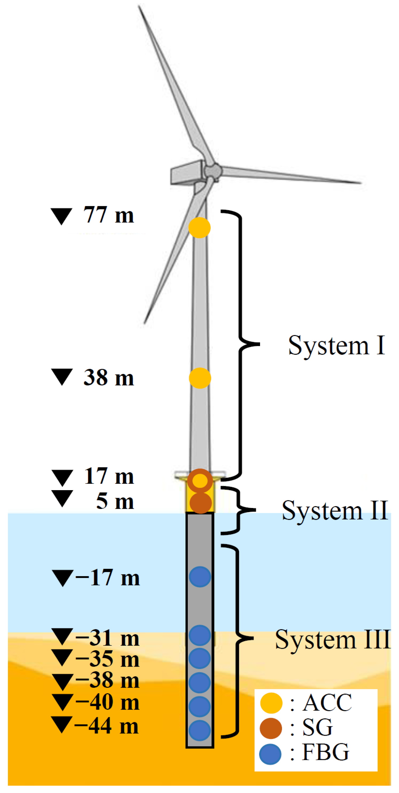
Between early 2017 and the end of 2019, the Nobelwind offshore wind farm in the Belgian North Sea hosted a measurement campaign on three of their turbines. The three turbines were selected with the goal to maximise the range of recorded vibrations and wind conditions. As a result, the turbines in the shallowest and deepest water were selected along with two on opposite edges of the farm and one at a corner of the farm. The basic measurement setup of all three turbines was the same seen in Figure 1, deviating only in the position of the sensors below water level to accommodate for different monopile (MP) designs and soil conditions. All sensors are separated into three separate systems for data acquisition. System I contains accelerometers on three levels of the turbine tower. Also included is one level of electrical strain gauges on the transition piece (TP). A second strain gauge level on the TP features its own system. On the MP, four lines of fiber Bragg grating strain sensors (FBG) constitute system III. Each of these optical fibers is grated at several levels with a focus on the area around the mudline. This dataset provides unique insights in the sub-soil strain response. While accelerometers could be installed and maintained freely, the optical fibers had to be mounted on the MP prior to their installation in 2017 and remained there after the completion of the measurement campaign. While not all fiber lines survived pile-driving, the majority of sensors recorded strains over a time of three years. For more details see [8]. The measurement data is complemented by environmental/operational data, e.g., wind speed, yaw angle, so-called SCADA data once every 10 min.
While the separation of measurements into independently working sub-systems was necessary for practical considerations. It also posed a challenge, as clock drift occurred between the three systems. It is therefore not guaranteed that measurement data of the three systems is recorded at the same time instance. In order to correctly combine data from the different systems and assess the accuracy of the proposed expansion methodology, it was essential that the clock-drift was resolved in post-processing. Therefore, a strategy is developed modifying timestamps of systems II and III to regain a global measure of time which is explained in [9].
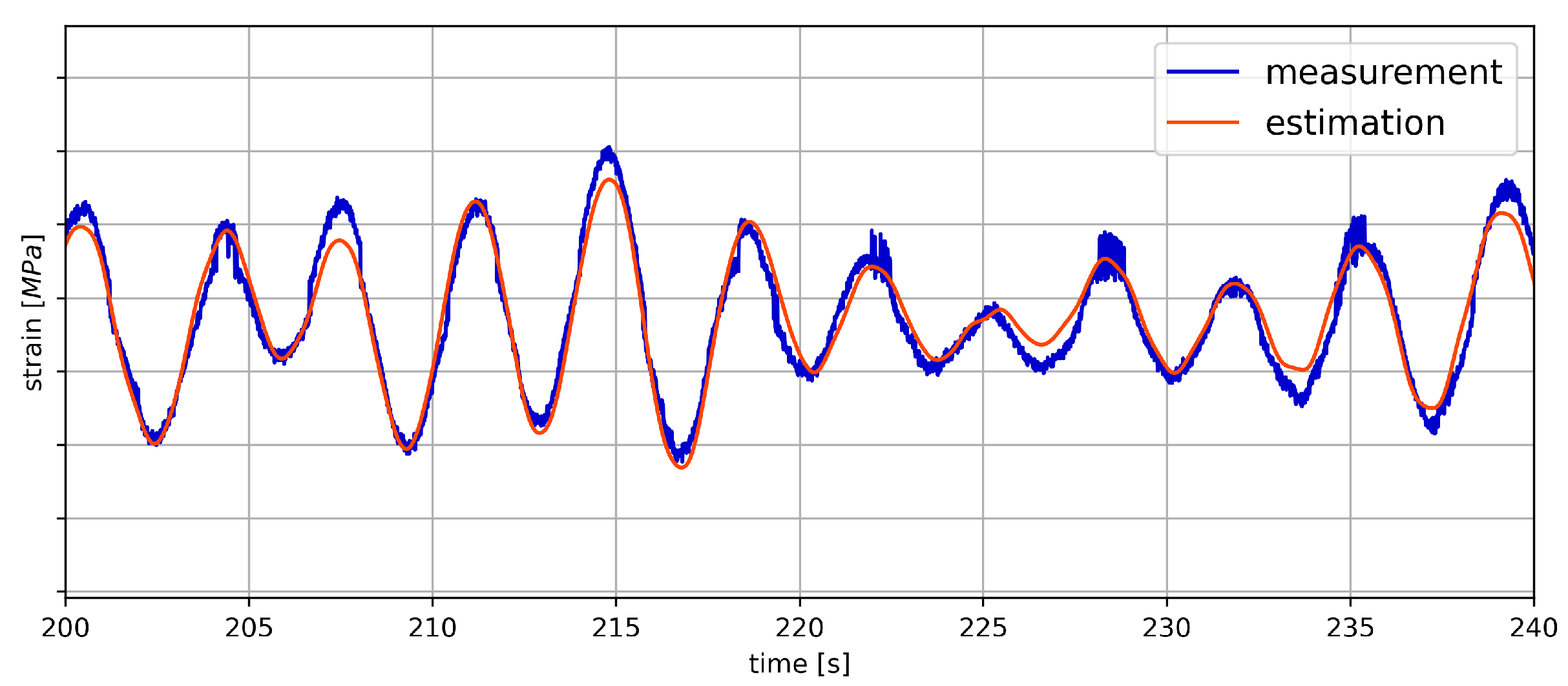
A second challenge was presented by a particular failure mode of FBG sensors. In normal operation, a FBG sensor reflects a single wavelength indicating the degree of strain it is experiencing [10]. However, when the grating is damaged, multiple wavelengths may be reflected by the sensor, this issue is referred to as peak-splitting. Since the current interrogator does not distinguish between multiple reflections, recorded fiber measurements can contain random jumps between a physical and erroneous strain level as seen in Figure 2 and introduce errors in any derived fatigue metric.
The goal of this research is to learn about fatigue progress by reconstructing strain history, validating the predictions using the FBG measurement data. Figure 2 therefore also contains the same time series estimated via virtual sensing (see Section 2.2.1). While easy to spot with the eye, the difference between the measurement and the virtual sensing result is non-negligible and FBG signals with peak-splitting should be omitted from any further analysis. The amount of measurement data collected in the three years makes some kind of automated anomaly detection necessary, which is described in detail in [11]. The current approach ensures that the FBG data used for validation within this paper is free of peak splitting and guarantees the physicality of the measurements. Also note, that this contribution only uses the data of one turbine.
2.2. Virtual Sensing
The goal of this research is to learn about fatigue progress in critical locations. For monopile foundations, usually a weld close to mudline will accumulate the most damage and thus drive design. A direct measurement, as available at Nobelwind, is very rare, and is hard to maintain so alternatives are desired.
Virtual sensing is an approach to use a limited set of measurement data to synthesize measurement data in unmeasured locations employing some mathematical model. For the application to critical welds on monopiles, accessible locations on the tower are used for instrumentation while critical locations on the TP/MP are estimated. The two common virtual sensing techniques using response measurements are Modal Decomposition and Expansion (MDE) [12,13,14] and the Kalman Filter [15]. Kalman filter estimates states based on the dynamic modes and frequencies of a structural model and can include damping and noise to the model. In contrast, MDE uses the modal superposition principle and only relies on a set of mode shapes for strain estimation. A comparative study of Kalman filter-based methods and MDE on an operational wind turbine on a monopile foundation concluded comparable accuracy for both techniques [16].
2.2.1. Modal Decomposition and Expansion (MDE)
The core of MDE is the modal superposition principle, i.e., a linear subspace projection into a space spanned by the characteristic mode shapes. It is assumed that a time dependent combination of n mode shapes can describe any vibration of a linear mechanical system:
where is the vector with the components of mode shape i at measurement location m and is the time dependent participation or modal coordinate of . The first step of MDE, i.e., modal decomposition, is to start from measured vibrations at m locations: and solving for all n modal coordinates , here stacked into , assuming the mode-shapes are defined:
in which is the matrix concatenating the mode shapes. Interestingly, the pseudo-inverse operation implies a least-square regression.
Modal expansion starts from assuming modal coordinates are valid for the entire structure. An estimation of strain can thus be done for any location by combination with the associated mode shape components:
where is the mode shape matrix of n strain mode shapes at estimation locations p. and are the Laplace transformation and the inverse Laplace transformation, respectively. Strain is the spatial derivative of displacement. Assuming vibration measurement is an acceleration signal, a double integration is required which is performed on the estimated modal coordinates in the Laplace domain, resulting in the 1/s2 operation in Equation (3). However, a poor signal/noise ratio of accelerometers and numerical instabilities close to 0 Hz can result in erroneous displacement estimates. As such [16] proposes to use a lower bound for the acceleration data. The lower bound is situated well below the first structural mode, while sufficiently high to avoid exaggerated low frequency contributions. From the high-pass filtered acceleration data, the dynamic contribution of the strain extrapolation is obtained through Equation (3).
In the literature, different concepts [4,6] are found to account for strain accumulated below within a quasi-static band. They commonly mimic the idea of MDE by applying pseudo mode shapes to measurement data. This research uses the concept in [6] and modifies it to conform to a fully data-driven approach which is described in Section 2.3.2.
2.2.2. Fatigue Calculation
Virtual sensing estimates strains in inaccessible locations to monitor fatigue progress. While earlier work of the authors focuses on the correct reconstruction of single measurements in time and frequency domain [9], fatigue performance of the technique mainly relies on a high estimation quality of specific conditions long-term. In fact, the accurate reconstruction of more damaging conditions, e.g., high wind speed is preferred over a stable fit between strain signals over the entire range of environmental and operational conditions. Consequently only damage-related quality indicators are used to evaluate the long-term performance of MDE.
Given a stress signal with multiple stress magnitudes , each occurring times. The Palmgren–Miner rule defines the caused damage D as a ratio with the cycles to failure for each (see Equation (4)). Assuming the curve of curve being a m-th order polynomial, Equation (4) can be rewritten using the negative inverse slope m and the intercept of curve and N axis :
In order to obtain all , pairs of a signal, i.e., the fatigue spectrum, it is passed through a rainflow cycle counting algorithm. To compare the caused damage between different signals, a fatigue spectrum is condensed into a single value, the damage equivalent stress range (DES). It is calculated as the single stress range that with a pre-defined number of cycles causes the same damage as the actual fatigue spectrum. Substituting , in Equation (4):
and solving for :
gives the main quality indicator used in this publication. When the DES is applied to virtual sensing, usually the fatigue of a measured and a predicted signal are benchmarked. Therefore, the absolute error on DES:
is defined, where index m indicates the DES of a measurement and p is the DES of a virtual sensing result respectively. The absolute error is useful to conclude about the performance of MDE over different data sets of a single sensor. Conversely, the percentage error in Equation (8) is used to analyze the bias of the estimation model:
Within this contribution, DES/, , and are used to compare short-term strain signals, i.e., 10-min recordings. Additionally, various measurements of a single sensor are appended to obtain lumped values for mentioned parameters used to evaluate fatigue performance between different sensors.
2.3. Methodology
After introducing the general concept of MDE in Section 2.2.1 and providing measurement data as described in Section 2.1, this section provides information about the synthesis of both. Considering measurement sensors of different heading are used to estimate strain in an arbitrary direction the Fore-Aft (FA)/Side-Side (SS) system is used as an intermediary step to assemble the estimations. Following [6], a dual-banded version of MDE is used. This way, dynamic and quasi-static bending moments in the FA/SS direction at target height are reconstructed according to Section 2.3.1 and Section 2.3.2 respectively, before the combined bending moment is transformed into the strain of an arbitrary direction in Section 2.3.3. The availability of measurement data over the entire length of the MP in this specific case might raise the question as to why an estimation algorithm is required altogether. However even if turbines would be covered with sensors, sensor failure or low measurement quality could be reasons to look for redundancy. In addition, common strain sensors have a life expectancy of only a few years making an estimation algorithm desired for fatigue assessments and life time extrapolation of the turbine.
2.3.1. Estimation of Dynamic Bending Moments
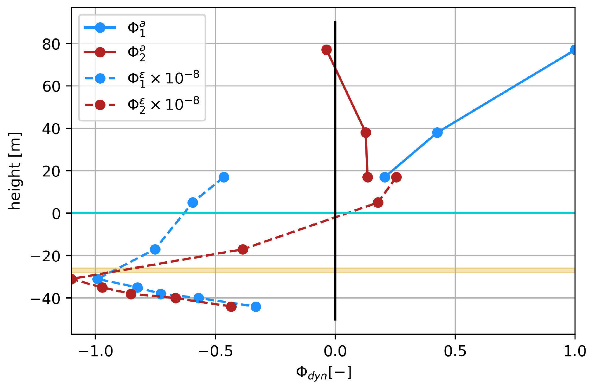
Modal decomposition and expansion method relies on a set of mode shapes. These can be obtained either from (updated) numerical (FE) models of the assets or directly from measurements. The first option is preferred giving a set of continuous mode shapes over the entire structure. The latter extracts mode shape values at measurement locations via operational modal analysis (OMA). The availability of measurement data over the entire length of the MP in this specific case however favors the data-driven approach avoiding any errors in the numerical model. Considering acceleration data is used to estimate dynamic strains, the mode shape matrix will contain different quantities. In [17], acceleration and strain measurements on a hull girder of a slender ship are used in combination to obtain displacement mode shapes via OMA. The research shows a better accuracy of mode shapes from combined data over mode shapes from strain as long as data are normalized properly. In this work, acceleration and strain data are first transformed from sensor direction into the FA/SS system. Therefore, a linear transformation matrix in is applied to two acceleration signals of perpendicular orientation. Before applying OMA to the combined data, accelerations are integrated into displacements and strains transformed into dynamic bending moments. Mode shapes are obtained from data in side-side direction using the PolyMAX algorithm [18] and are assumed valid around the circumference. As seen in Equation (2), the number of considered modes is limited by the number of measurement locations. Due to the low frequent nature of strain only the first two bending modes are used and the effect of modal truncation on the fatigue estimate is assumed small. The inclusion of higher modes could even have a detrimental effect, considering the deteriorating signal/noise ratio of strain gauges for higher frequencies. Measurements of a single 10-min interval under rated power with a wind speed of ms−1 are used to obtain the set of mode shapes for all estimations. This simplification thus assumes linearity over the entire load spectrum. MDE in the time domain requires real mode shapes, thus the imaginary part of the mode shapes are ignored. As the system is relatively lightly damped, this imposes little drawback. Figure 3 shows the resulting mode shapes.
Excitation from wind and wave is (partially) situated below the first natural frequency of the turbine structure resulting in quasi-static deflections. Due to the loading being in fact not or only partially dynamic, mapping to a set of dynamic mode shapes is a known problem. In [4], the MDE technique is applied to a tripod structure in order to reconstruct the full-field strain history. Strain from wave loading is reconstructed by a set of so-called Ritz-vectors, i.e., operational deflection shapes (ODS), which can be obtained from numerical models or via frequency domain decomposition [19]. The conceptional difference to dynamic modes is the dependence of ODS on the input location of exciting force. Looking back at Equation (3), this equation is agnostic of the position of any force, and this information has to be carried within . Which actually means that are more closely related to operational deflection shapes (ODS) than to pure mode shapes.
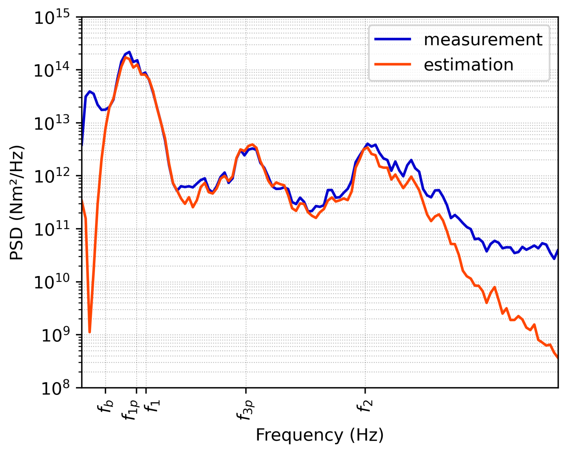
Due to the issues of exaggerating noise at very low frequencies, the accelerometers are only considered above Hz in the dynamic band. As a result, the slow-varying wind thrust has to be estimated separately, which is covered in Section 2.3.2. Conversely, wave loading is closely spaced to the first natural frequency and has to be mapped by the MDE method. Fortunately the extraction of mode shapes from measurements via OMA partially resolves as the experimentally-found mode shapes are also influenced by the localized presence of the wave loading. Figure 4 illustrates the accurate reconstruction of the dynamic bending moment below the first natural frequency , also indicating vibration from rotor harmonics and . Finally, note the low spectral density beyond the second mode confirming the choice to limit the method to the first two modes.
2.3.2. Estimation of Quasi-Static Bending Moments
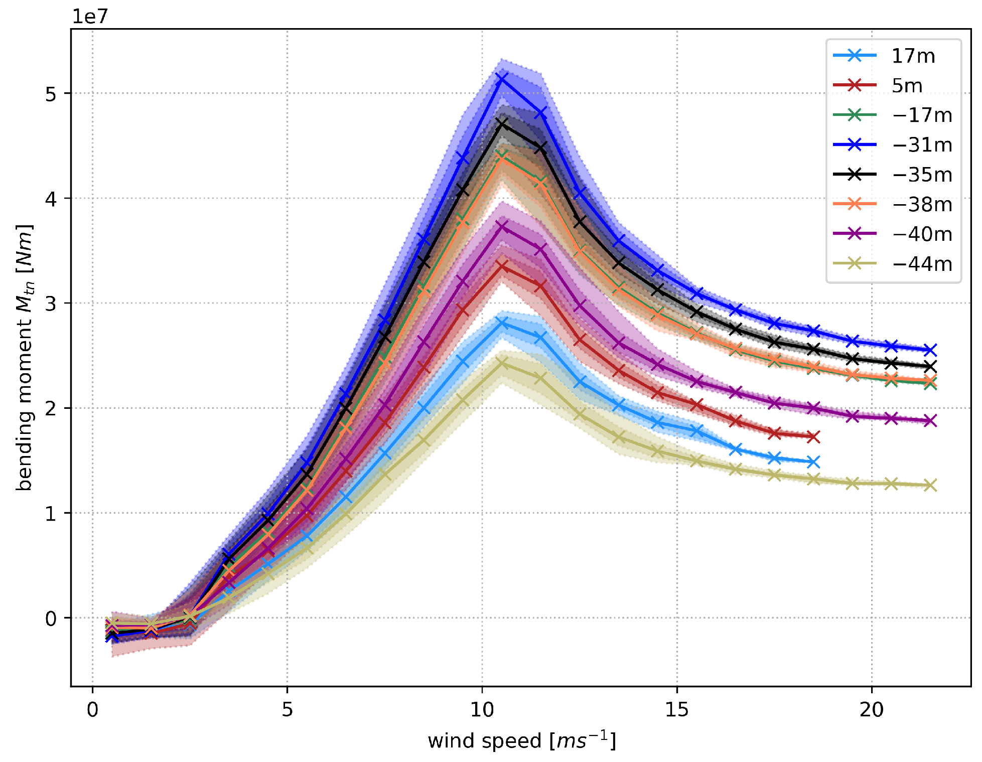
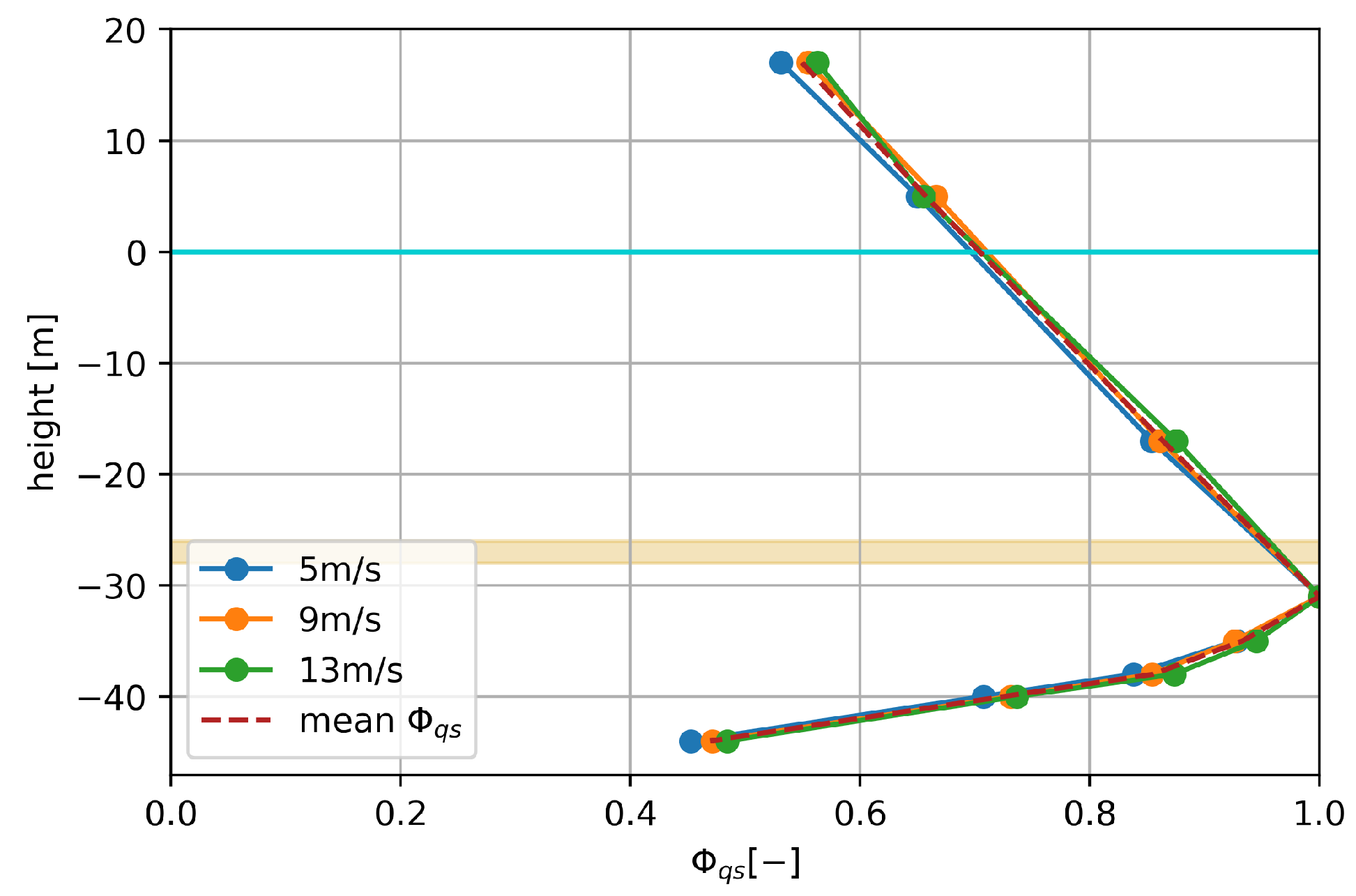
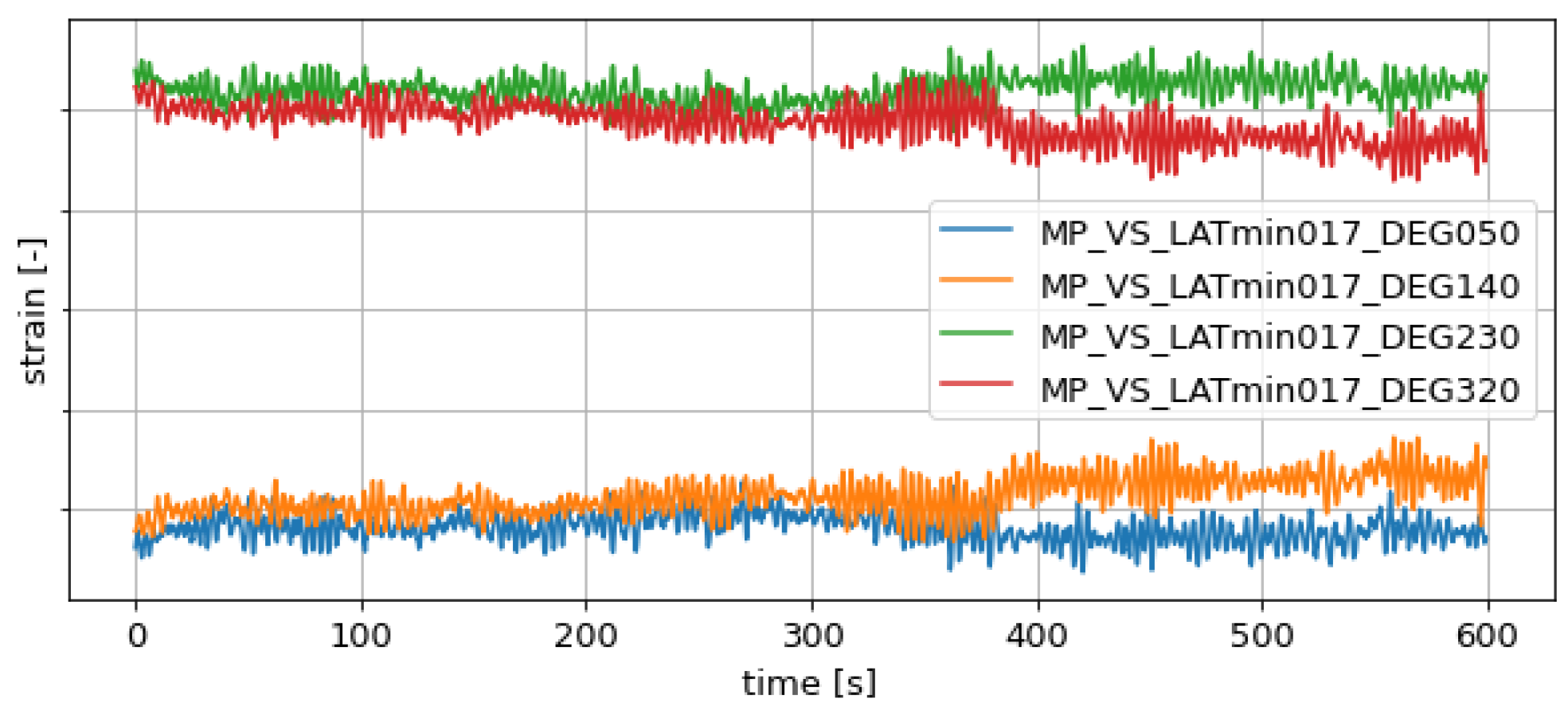
Displacement or its spacial derivative strain is a low frequent phenomenon. While considerable acceleration may be present at higher frequencies, the impact on strain will be limited. With fatigue being correlated to the strain history, emphasis is placed on the accuracy of virtual sensing in the quasi-static band below . A single level of strain gauges on top of the TP is used to estimate strain for this frequency band. The boundary frequency to the dynamic band is chosen to 0.1 Hz in an attempt to separate low frequent wind thrust from wave and rotor excitation. Filtering is performed by a forth-order Butterworth filter. With the first bending mode occurring outside the quasi-static band, MDE cannot be applied directly. As explained in Section 2.3.1 an ODS is used instead to estimate the quasi-static bending moment due to wind thrust. In [20], is found by subjecting a FE model with a horizontal force on the nacelle corresponding to the wind pressure and extracting the static deflection shape. Instead of employing a FE model in this work, is derived from bending at 0 Hz. Therefore, strain measurements of all levels are used to calculate bending moments in the Fore-Aft direction, i.e., . The searched pseudo mode shape is found by calculating 10-min averages of these bending moments over a period of one year. While the bending moments vary with varying environmental conditions, the ratio of bending moments between different heights show little dependency from environmental conditions, e.g., wind speed which is illustrated in Figure 5. Pseudo-mode is found by taking the ratio between the bending curves of the different measurement locations. Calculating for different wind speed ranges shows a stable ratio for wind speeds above cut-in as seen in Figure 6.The remaining spread between the shown curves is explained rather with measurement uncertainty over physical reason. Therefore, it was decided to use an averaged instead of a mode shape dependent on the environmental condition avoiding an over-fit of the model. Below cut-in wind speed, measured quasi-static strains are more affiliated to the off-center center of gravity of the nacelle and random measurement noise and can be neglected. The expansion step is basically scaling the quasi-static pseudo mode shape with the measured bending moment at the TP :
where index p indicates unmeasured locations.
2.3.3. Full-Field Strain Reconstruction
Quasi-static and dynamic bending moments are calculated in the FA/SS direction of desired height and superimposed subsequently. The final step is the transformation of the estimated , in an arbitrary direction accompanied by back-transformation into strain. Bending moments from the FA/SS system are transformed into , by rotating the coordinate system into arbitrary direction by employing the linear transformation matrix:
The normal strain is found by:
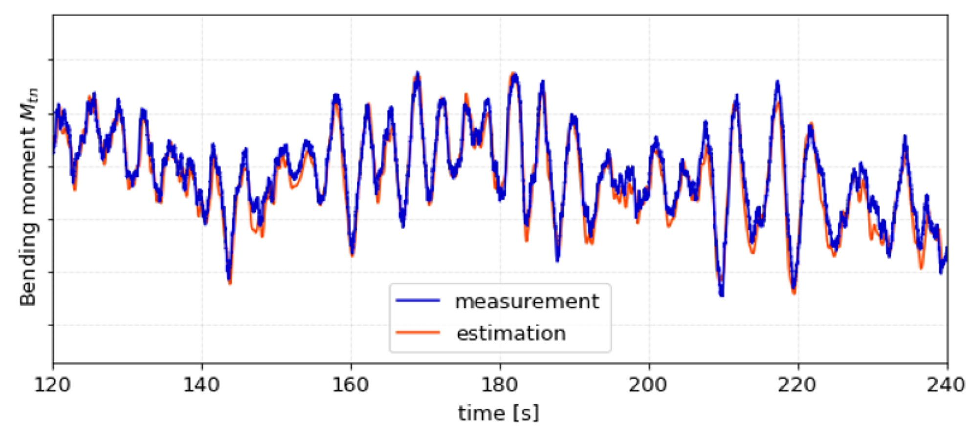
considering a bending strain at location 1 in a coordinate system with axes is caused by orthogonal bending moment in direction 2. R describes the inner radius of the MP, is the area moment of inertia, and E is the Young’s modulus. A look into sample time series as shown in Figure 7, Figure 8 and Figure 9 confirms a high prediction accuracy. Aligned with the wind direction, (see in Figure 7), shows more low-frequent oscillations coming from variations in the thrust loading. The good performance is largely a result of a well-calibrated quasi-static band.
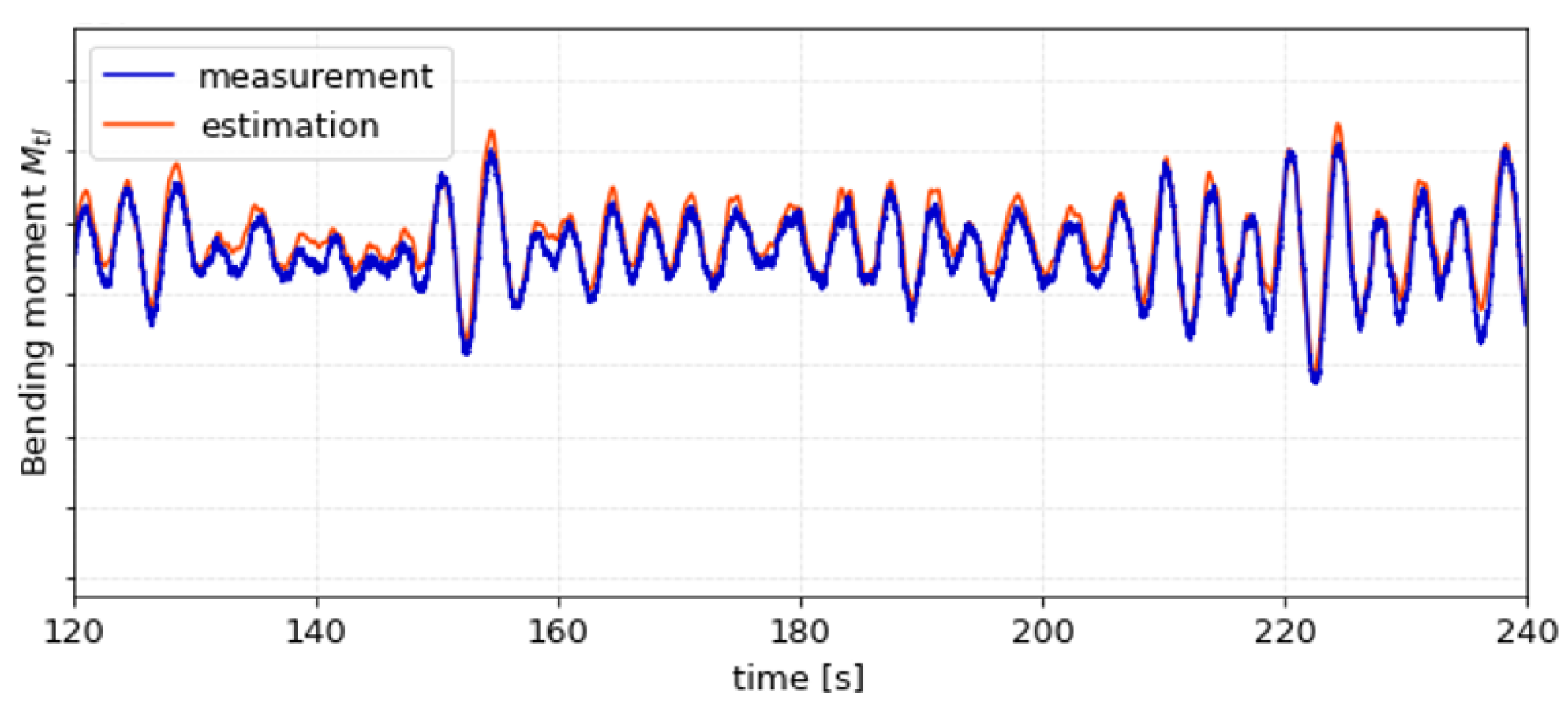
Conversely, in the SS direction, i.e., cross-wind, oscillations are primarily driven by the first mode. The near perfect fit between measurement and estimation in Figure 8 confirms quality of the mode shapes obtained via OMA.
When transforming into a strain of any arbitrary direction, contributions from both FA and SS are mixed in a ratio depending on the prevailing wind direction and the chosen direction as illustrated by Figure 9. Note, that neglecting the acting normal force N in Equation (10) leads to an offset of the strain after transformation compared to the reference system.
3. Results
Virtual sensing is applied to long-term acceleration and strain data from tower and TP to estimate strain of arbitrary direction on the substructure. This section describes the validation of MDE accomplished by the use of acceleration measurements on the tower to reconstruct dynamic strain and strain measurements on the top of the TP (17 m ) to estimate quasi-static strain. Validation sensors are chosen on the bottom of the TP and on the submerged and sub-soil parts of the MP. Then estimations are bench-marked with measurements in terms of fatigue. While earlier publications are focused on the accurate reconstruction of 10-min timestamps [11], the long-term fatigue performance is investigated here. Therefore, in line with the S/N curve D with , for free corrosion as defined in [21], with no stress concentration factor is assumed for the calculation of DES at all locations for the sake of simplicity.
3.1. Validation Data
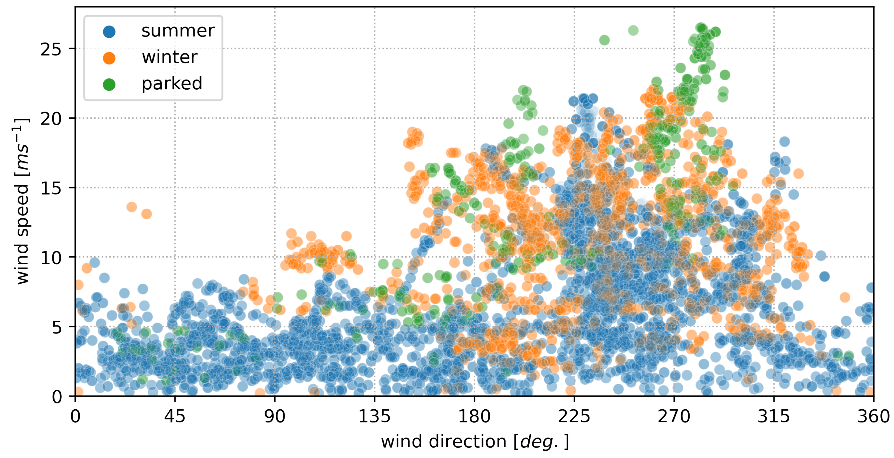
Three validation sets are composed with a total number of 25,405 samples to represent the full spectrum of environmental and operational conditions. One set contains mostly rotating conditions from two subsequent summer periods. To investigate how seasonal effects influence the accuracy of MDE, another validation set with data from one winter is added. A third set covers exclusively parked conditions. All sets contain data from a total of 13 different sensors as listed in Table 1 which will be benchmarked with corresponding predictions in the following section. Figure 10 shows that all three validation sets contain a wide range of environmental conditions. A big portion of samples is recorded during idling and run-up states of the turbine. These samples show the biggest diversity in wind direction. The summer set features most of those low wind conditions. Conversely, samples from rated conditions usually occur for wind directions between 200 and 300 deg. While samples with high wind speed can be found in every validation set, the biggest share of rated conditions is recorded in the winter set.
Table 1 gives information about the number of samples per sensor and per validation set. By far, most samples are taken during the summer periods with the parked set consisting of only 8.5% of the total number of samples. A share of the FBG measurement data on the MP is corrupted by peak splitting as described in Section 2.1 and cannot be used to evaluate the quality of virtual sensing without additional pre-processing. Samples for the monopile were handpicked to not contain peak splitting, resulting in a lower number of samples per sensor for MP locations while sensors on the TP are electrical strain gauges and are thus not affected. Due to the small number of samples, estimation is forfeit at sub-soil levels −40 m and −44 m.
3.2. Fatigue Assessment
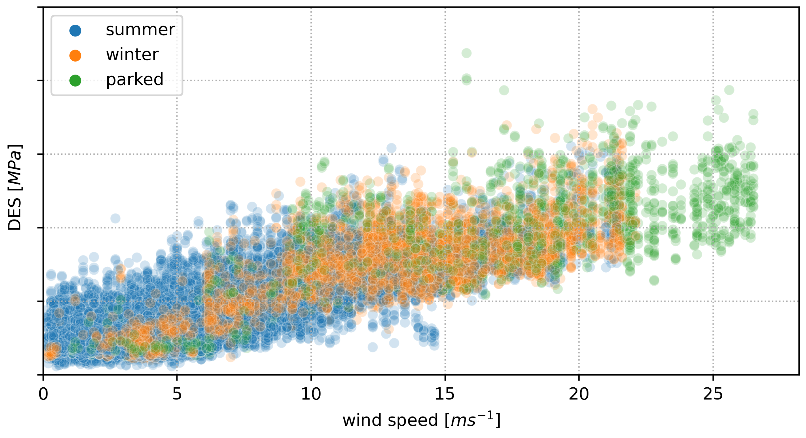
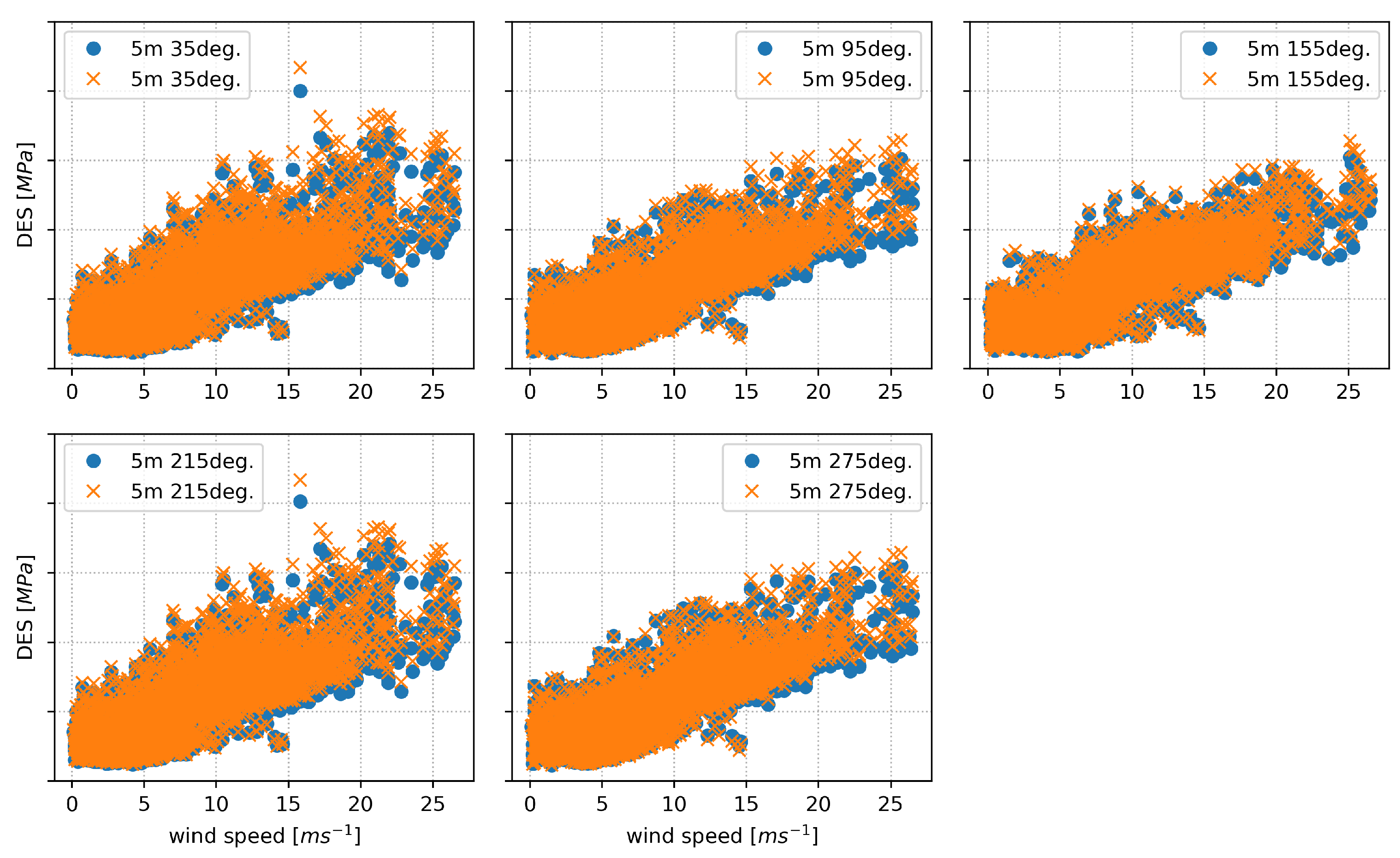
This section focuses on the damage accumulation of virtual sensors and analyzes the accuracy of a fatigue estimation. To be able to compare damage inflicted by different fatigue spectra throughout this section, the metric damage equivalent stress range (DES) is used (see Section 2.2.2). In Figure 11, the distribution of measured DES versus wind speed of all sensors combined is shown. Fatigue damage clearly correlates with wind speed, however the relationship appears to be not strictly linear. For low wind speed, i.e., idling and run-up conditions, the DES grows steadily and for rated conditions, the fatigue increase slows down. Similar findings are described in [22] for joints of jacket foundations.
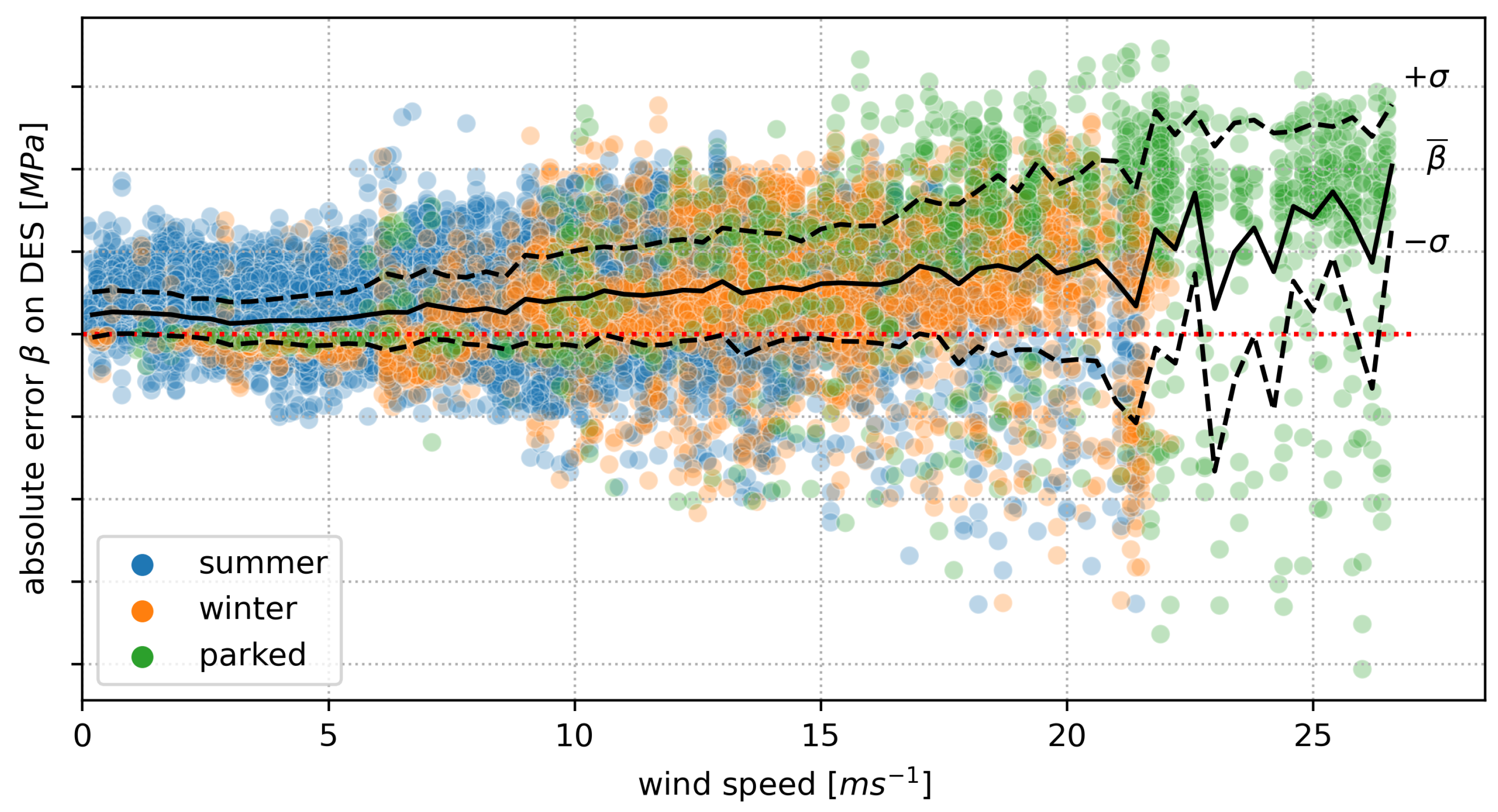
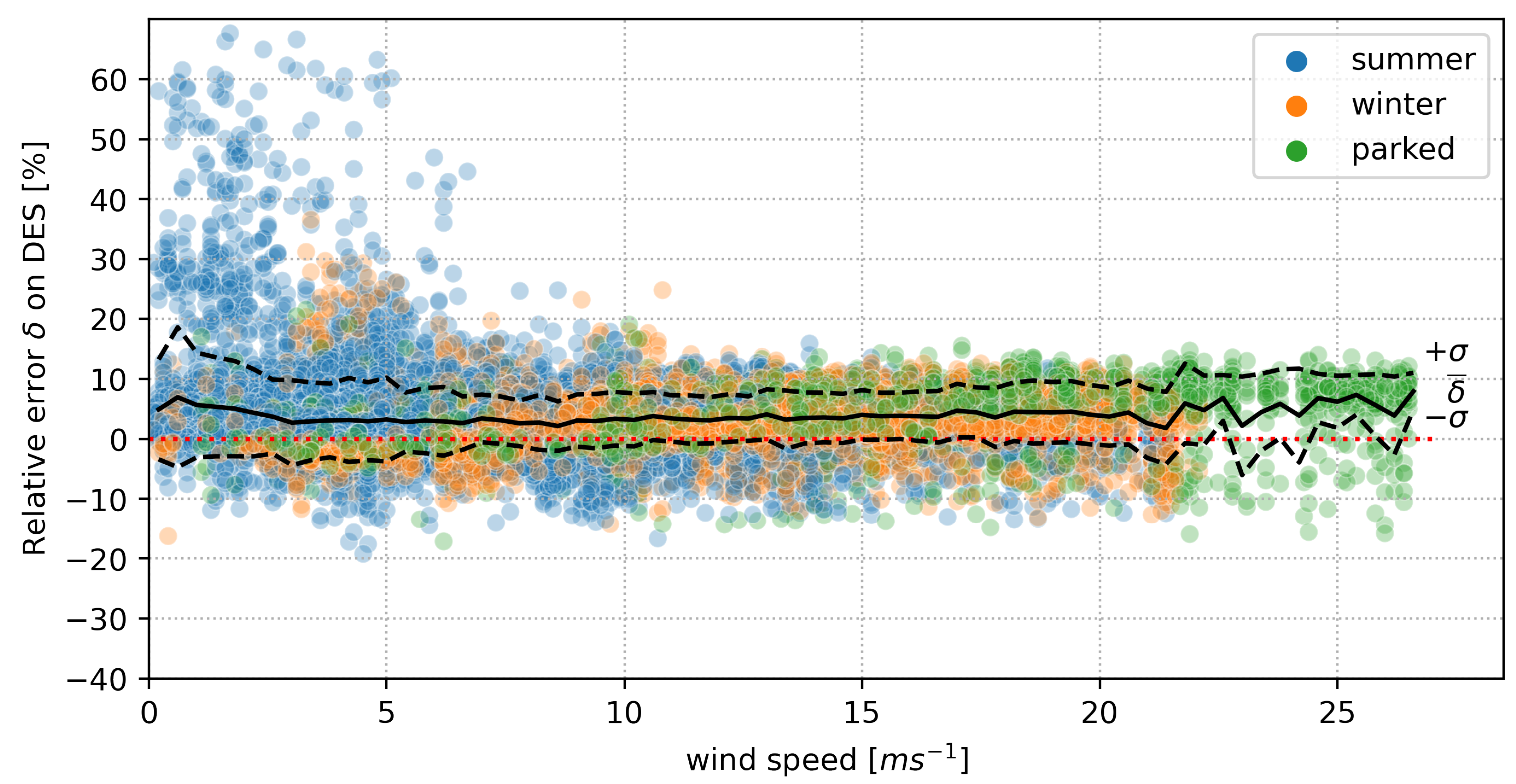
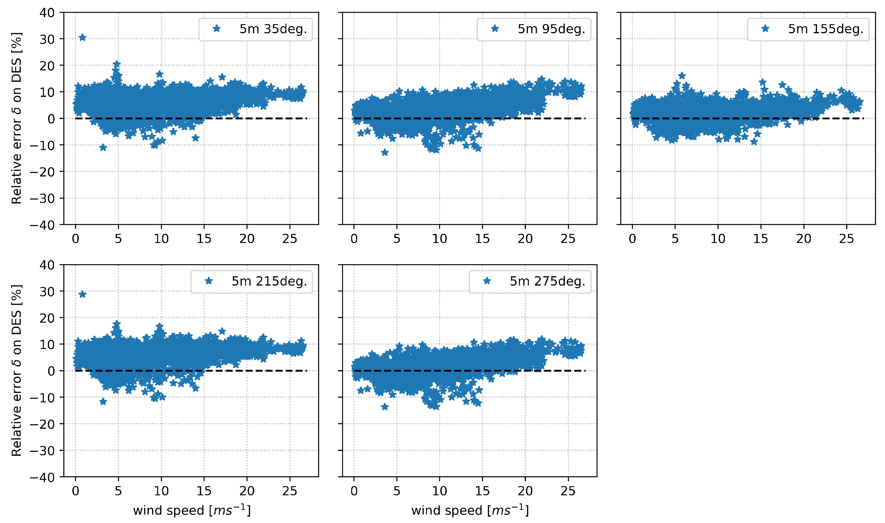
The comparison of stress ranges from measurements and estimations is illustrated in Figure 12 in terms of absolute error and in Figure 13 for relative error. As indicated by the increased fatigue at a higher wind speed, the absolute error grows with wind speed. The average error being slightly bigger than zero for low wind also grows with wind speed, revealing a bias of the estimation. The standard deviation grows proportionally but also indicates different behavior for extreme wind speed: First, before cut-in mean error and standard deviation appear independent from wind speed. Secondly, for wind speeds exceeding 20 ms−1 both parameters are unstable due to a lack of samples. These two regions can also be found in Figure 13 describing the relative error . Conversely to the mean relative error and its standard deviation are elevated below cut-in dropping to a stable level for run-up and rated wind speeds before becoming unstable for high wind speed as described above. Fatigue is slightly overestimated over the entire range of wind speeds and estimations at low wind smaller than 7 ms−1 appear more prone to outliers.
The worse performance of MDE at low wind speed is mainly due to two effects: First, the signal to noise ratio is generally worse where absolute values of measurements are smaller. Comparing a noisy measurement with a MDE estimation results in a worse fit while this is no shortcoming of the estimation model but of the measurement. Second, as described in Section 2.1, SCADA data, e.g., yaw angle are updated once every 10 min. The estimation procedure includes the transformation of measurements into a FA/SS system before extrapolating the data. Low wind speeds generally entail more frequent yawing action, resulting occasionally in input data that is not transformed properly.
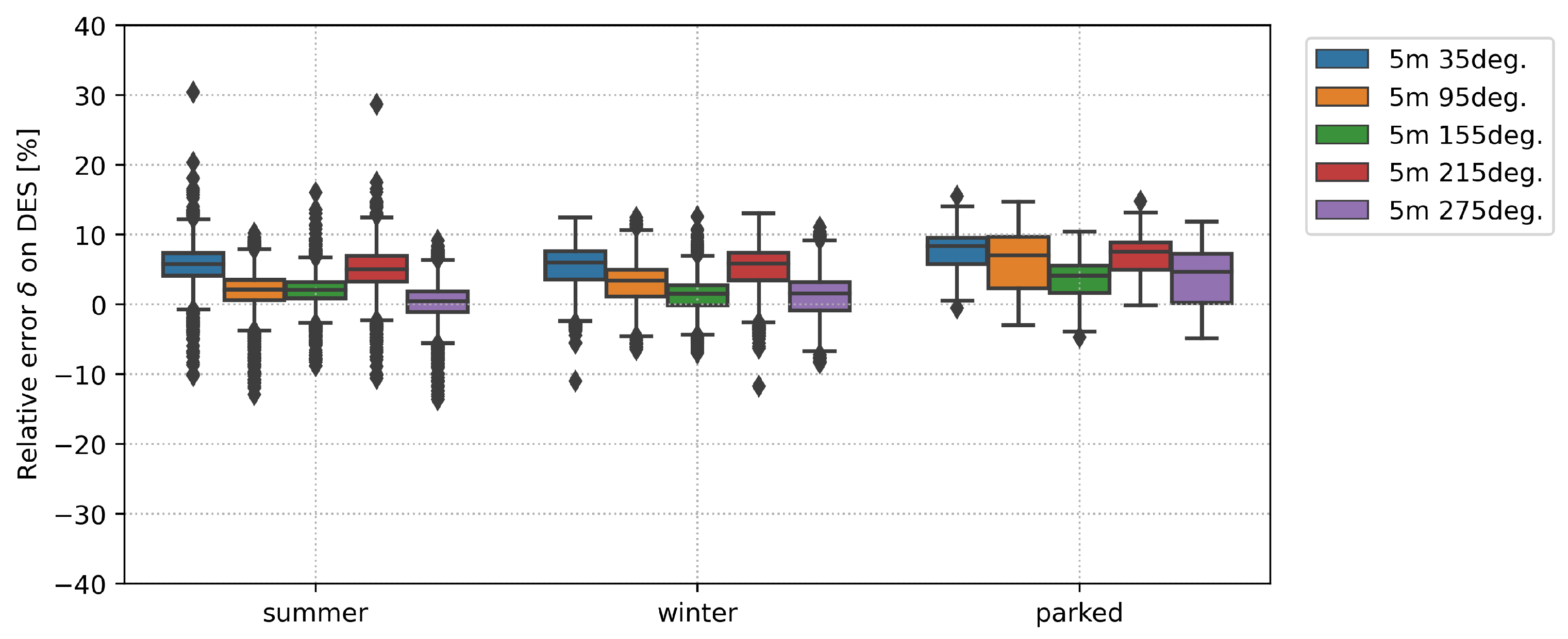
The error on fatigue clustered for the three validation sets already revealed general trends of the estimation model. Adding information from Table 1 helps to understand that those trends are mainly experienced by the TP sensors. Due to the small portion of validation data from MP sensors, MP specific effects are hard to spot in the previous figures. Therefore, the relative error per sensor and validation set is analyzed in Figure 14 and Figure 15. Box and whisker plots illustrate the spread of data by height of the box consisting of 50% of the data and whiskers showing the quartiles. If outliers are detected, these are shown separately. TP sensors in Figure 14 show good performance by only slightly overestimating fatigue with an error of max. 7.05% for the sensor at 5 m oriented towards 35 deg. Sensors on the TP are set up in opposing pairs and these pairs behave similarly in terms of relative error . Both worst performing sensors are in direction 35/215 deg while remaining sensors on the dry part of the structure show a mean error of less than 3% on DES. Analyzing data spread per TP sensor and validation set reveals different effects: On one hand, the box height increases from summer over winter to the max. value in the parked set. So the 50% of data closest to are estimated with the least uncertainty in summer and with the highest level of uncertainty in the parked set. Again going back to Table 1 leads to the assumption that an increase in number of samples for the parked set has the potential to diminish this uncertainty compared to the other validation sets. On the other hand, whiskers are comparable in height over all sensors and sets, however, by far, most outliers are found for the summer periods. Outlier conditions are assumed to be subject to yawing actions, which can reduce the estimation quality due to the current low sampling rate of SCADA data. In terms of mean error, sensors behave in a stable condition over all validation sets and mean error of opposing sensors is similar. Appendix A Figure A3 shows that the higher of sensors at 35/215 deg is coming from a slightly worse performance at a low wind speed while a general estimation bias is shared by all TP sensors. Overall, it is found that DES on the TP is slightly overestimated with the error being mainly influenced by the sensor location and behaving very stable for different validation sets.
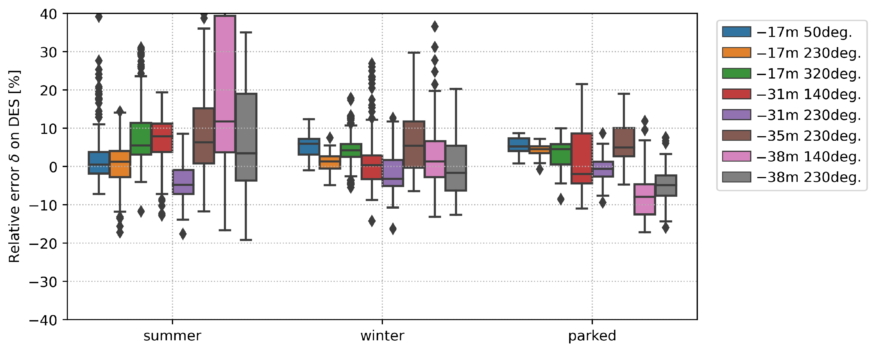
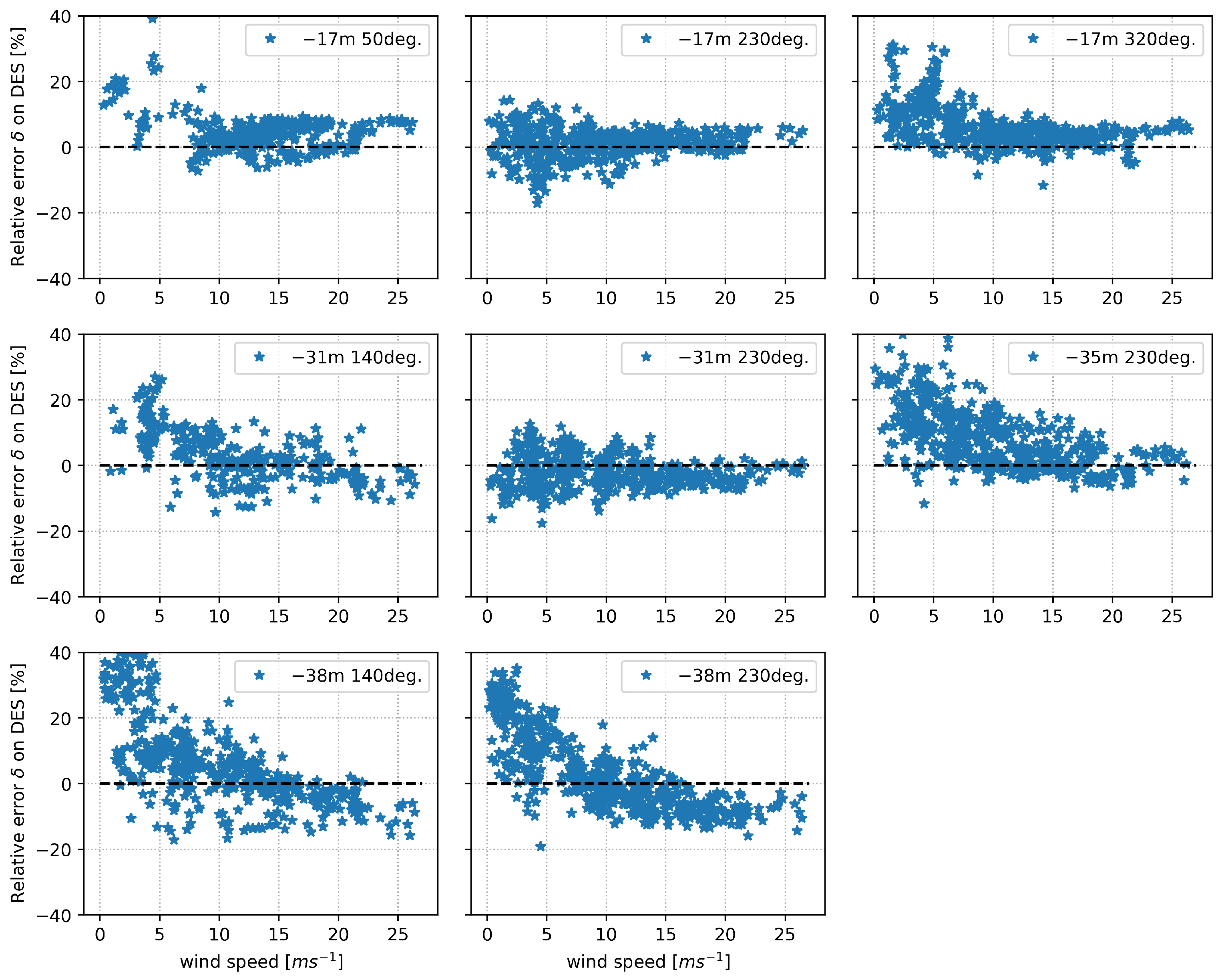
The MP features sensors on the submerged part, i.e., −17 m and sub soil. In general, submerged sensors perform better than sub-soil sensors while both show a higher variance of the relative error on DES compared to the dry part of the turbine structure. It is striking that contrarily to TP sensors, no MP sensor shows a similar behavior in terms of mean error or data spread over different validation sets. The summer periods show consistently the largest variations for both and data spread. Consulting Table 1 allows one to draw conclusions between box height/ and number of samples. For the TP, it is shown that a high number of samples reduces the data spread, which is illustrated by the box height. In contrast to TP sensors, no positive correlation is found here, so even sensors with most samples do not have more stable error characteristics, e.g., shrinking box height, smaller whiskers, etc. Addressing the variance in estimation accuracy, it is important to stress that MP sensors all have unique sets of samples. For MP sensors, low wind conditions show significant spread on as seen in Appendix B, meaning that sensors with a large number of samples in low wind perform worst. This trend is most significant for summer clusters of sensors at −38 m. Thus differently to TP sensors, error characteristics are not simply driven by the sensor location but also by the validation set, i.e., considered environmental and operational conditions. Interestingly, Figure A4 shows that MP sensors except sub-soil sensors at level −38 m estimate strain with a smaller estimation bias than TP sensors. It is envisioned that a different distribution between samples of high and low wind speed has the potential to reduce on the MP. The observed variations of and are also assumed to converge or to stabilize with a higher number of samples.
While the sample-wise error analysis emphasizes the error coming from low wind conditions, the accumulated fatigue remains small (see Appendix A). To obtain more representative values for , Table 2 calculates the relative error on DES for all samples per sensor combined. At the TP, again sensor at 5 m oriented towards 35 deg performs worst with of 7.05%. In contrast, MP sensors perform much better than in the sample-wise analysis. Most notably, sensor −38 m 140 deg, which was earlier named as one of the worst performing sensors, reaches an error of only −2.62% on DES.
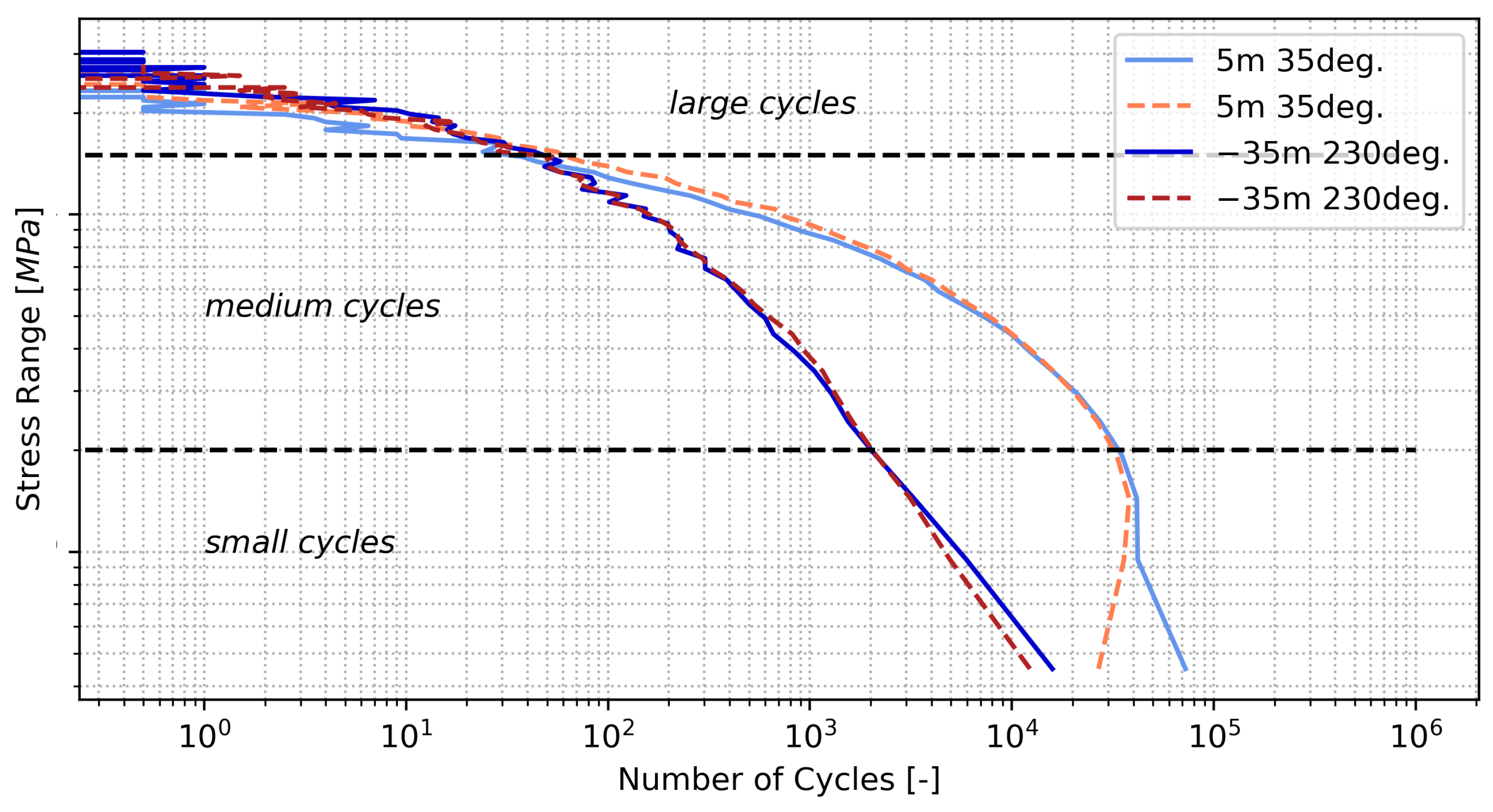
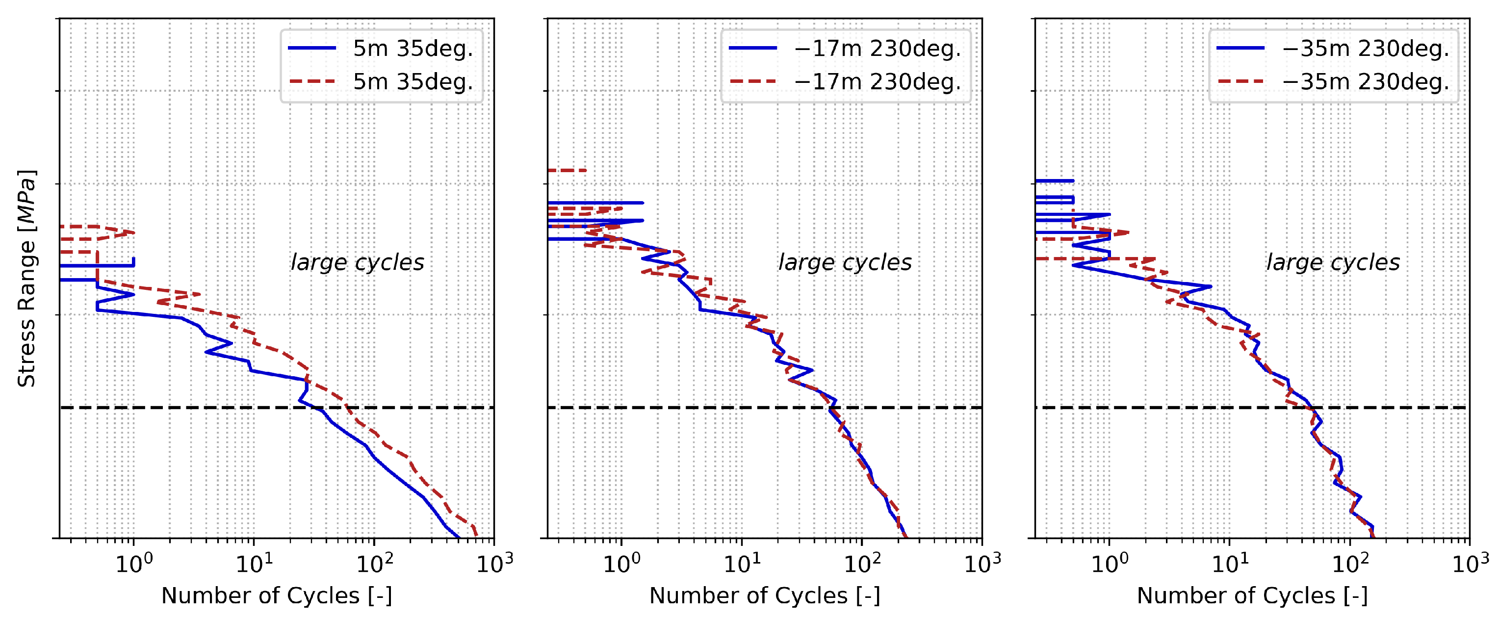
Figure 16 shows fatigue spectra of the worst-performing TP sensor and a sub-soil sensor close to the location of max. bending. Fatigue spectra of all sensors are gathered in Appendix C. Low wind conditions accumulate cycles of small stress ranges while conditions with strong wind and wave activity lead to the small number of cycles on top of Figure 16. In general, three different areas can be distinguished: The area of small cycles, where the number of cycles is underestimated. On one hand, a systematic underestimation is expected due to simplifications in the estimation model, e.g., modal truncation. On the other hand, noise in strain measurements will lead to an increased nonphysical cycle number. Then the area of intermediate cycles, which shows a mostly good fit between measurement and estimation. Finally, an area of large cycles can be distinguished. While only assembling a small number of cycles, the importance for fatigue is not to be underestimated. For instance, the shown MP sensor contains 71.1% of samples in the area of small cycles accounting for 17.6% of DES while less than 1% of cycles compose the area of large cycles accounting for 69.2% of DES.
To illustrate deviations in the large cycles in detail, Figure 17 shows a zoom into the fatigue spectra of sensors in the dry zone, submerged zone, and sub-soil zone. The measurement spectrum of the TP sensor is shifted upwards resulting in a simple scaling of larger stress cycles. This represents the estimation bias found in the sample-wise analysis. The worst performing sub-soil sensor at −38 m shares both orientation and error characteristic. In Section 2.3.1, it was described that mode shapes are obtained at one specific orientation and assumed valid circumferentially. This simplification combined with measurement variability is held responsible for the observed error and a correction of the corresponding mode shape components in can partially resolve it. Conversely, submerged and sub-soil sensors in Figure 17 show a more randomized error characteristic and no general bias. It appears that the error on fatigue mainly originates in the mismatch of a small number of large cycles. Considering the small number of samples for MP sensors, it is assumed that the relative error can be reduced by increasing the number of samples and is only partially due to systematic failures. Sensor −17 m 230 deg in the center plot of Figure 17 shows a slightly better fit for medium-sized stress ranges and catches the small number of large cycles, better resulting in an error on DES of only −0.86%.
4. Conclusions
This contribution presents a full-field strain reconstruction technique for offshore wind turbines on monopile foundations validated on real-world measurement data based on a data-driven and strongly simplified estimation model. The model is dual-banded combining a small set of acceleration measurements and the first two structural modes in the dynamic band and the static deflection shape of the turbine with a single level of strain measurements in the quasi-static band. After setting up the model, measurement data from the Belgian offshore wind farm Nobelwind is used to extrapolate strain measurements to submerged and subsoil locations on the turbine structure. The estimation accuracy is gauged over 25,405 samples taken from a multitude of environmental and operational states over the course of one year. While the model performs best for intermediate wind speeds between 7 ms−1 and 20 ms−1, increased variance is found for low and strong wind. Fatigue assessment of 13 locations placed on the dry, submerged, and sub-soil part of the structure on multiple levels and orientations shows a max. error on fatigue of 8.97% while the majority of sensors in all zones estimate fatigue with an error of less than 4%. It is shown that the worst performing sensors on TP and MP point in the same direction and share an estimation bias. While measurement variability cannot be ruled out as plausible cause, it is envisioned that additional validation data could help tune connected mode shape components to reduce the error on fatigue even further.
Author Contributions
Conceptualization, M.H., W.W., and C.D.; Formal analysis, M.H.; Funding acquisition, C.D.; Supervision, W.W. and C.D.; Writing—original draft, M.H.; Writing—review & editing, M.H., W.W., and C.D. All authors have read and agreed to the published version of the manuscript.
Funding
This work was conducted in the frame of the ICON SafeLife: Lifetime prediction and management of fatigue loaded welded steel structures based on structural health monitoring. Data for this project was collected during the O&O Nobelwind. Wout Weijtjens is a post-doctoral researcher funded by the Research Foundation-Flanders (FWO).
Institutional Review Board Statement
Not applicable.
Informed Consent Statement
Not applicable.
Data Availability Statement
The data is not publicly available due to confidentiality constraints.
Acknowledgments
The authors would like to acknowledge the continued support provided by Nobelwind NV.
Conflicts of Interest
The authors declare no conflict of interest. The funders had no role in the design of the study; in the collection, analyses, or interpretation of data; in the writing of the manuscript, or in the decision to publish the results.
Abbreviations
The following abbreviations are used in this manuscript:
| MP | Monopile |
| TP | Transition piece |
| FA | Fore-Aft |
| SS | Side-Side |
| FBG | Fiber Bragg grating |
| LAT | Lowest astronomical tide |
| OMA | Operational modal analysis |
| ODS | Operational deflection shape |
| MDE | Modal decomposition and expansion |
| DES | Damage equivalent stress range |
Appendix A. Damage Equivalent Stress Ranges
Figure A1.
Sample-wise damage equivalent stress ranges for sensors on the TP with measurement (dot) and estimation (cross).
Figure A1.
Sample-wise damage equivalent stress ranges for sensors on the TP with measurement (dot) and estimation (cross).

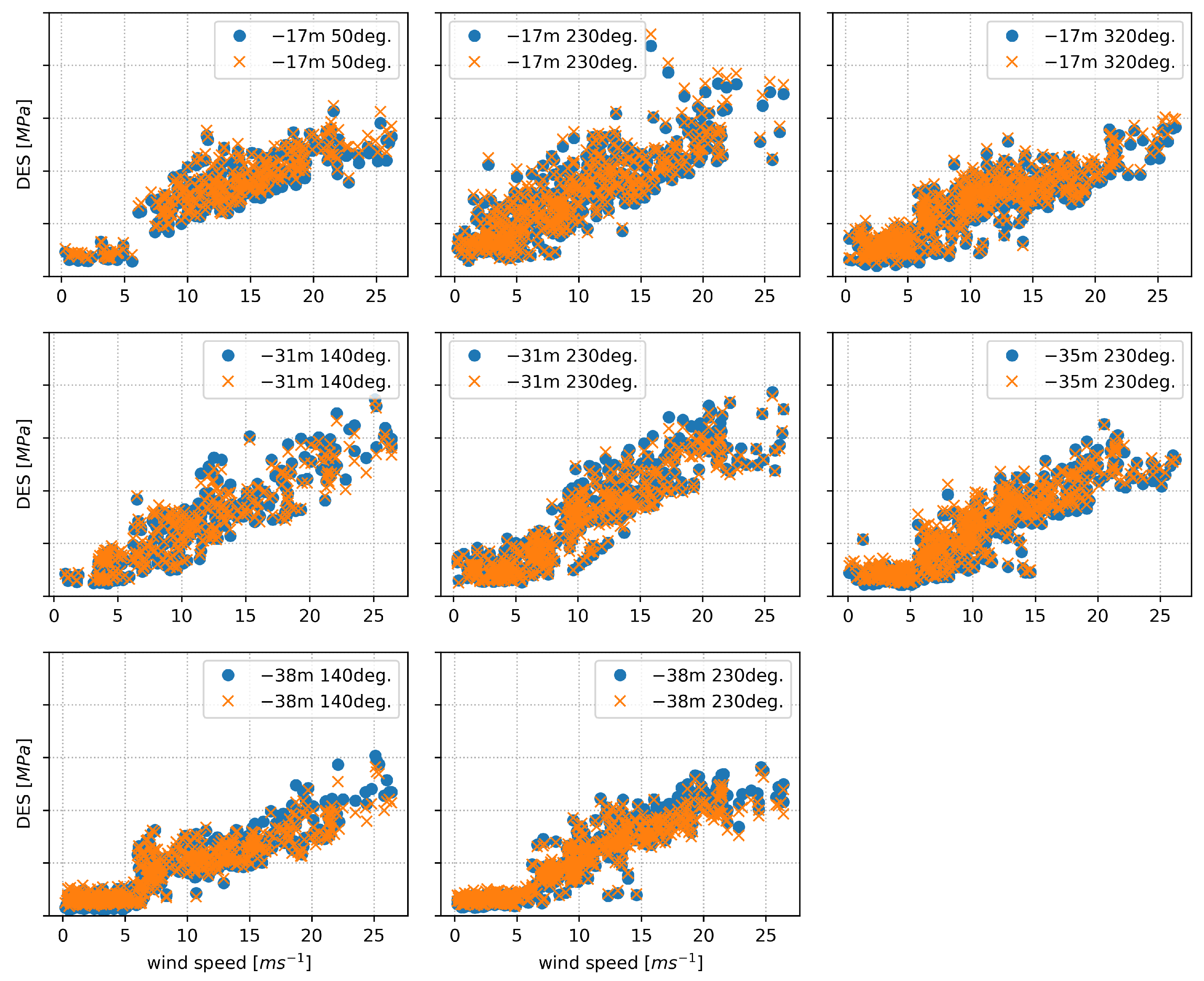
Figure A2.
Sample-wise damage equivalent stress ranges for sensors on the MP with measurement (dot) and estimation (cross).
Figure A2.
Sample-wise damage equivalent stress ranges for sensors on the MP with measurement (dot) and estimation (cross).

Appendix B. Relative Error δ on DES
Figure A3.
Relative error on DES for sensors on the TP.

Figure A4.
Relative error on DES for sensors on the MP.

Appendix C. Fatigue Spectra
Figure A5.
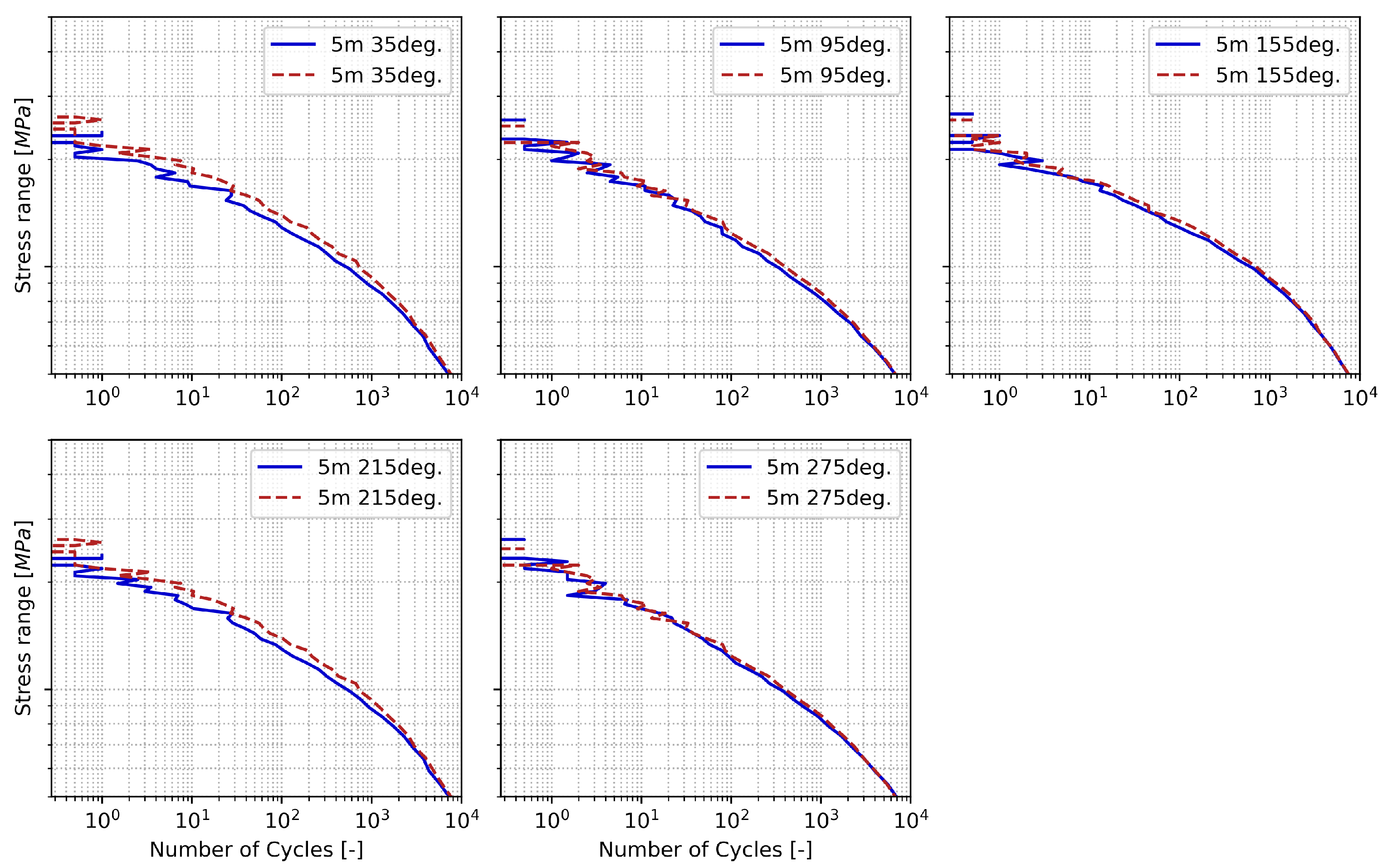
Zoom into fatigue spectra for sensors on the TP with measurement (solid) and estimation (dashed).
Figure A5.
Zoom into fatigue spectra for sensors on the TP with measurement (solid) and estimation (dashed).

Figure A6.
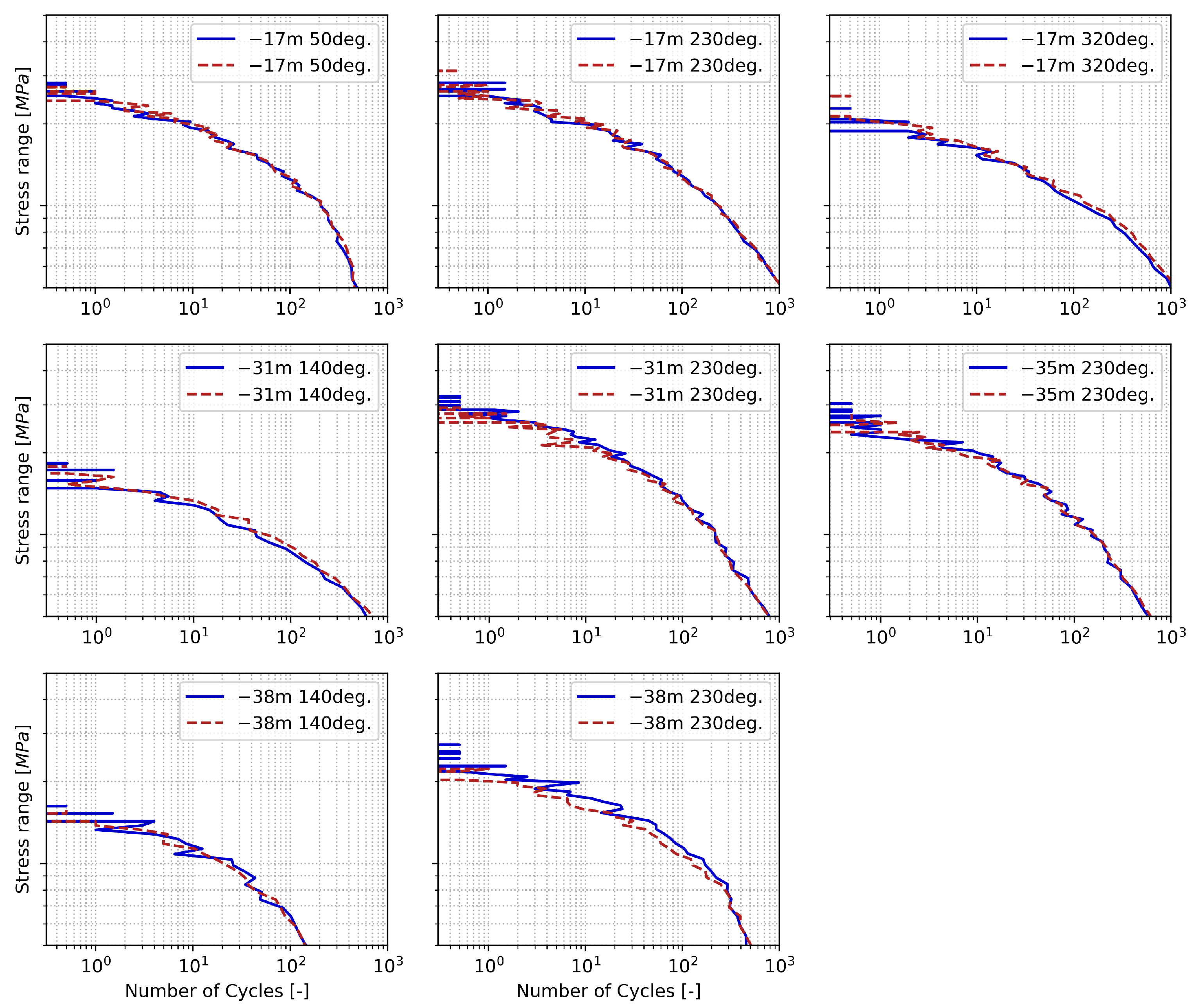
Zoom into fatigue spectra for sensors on the MP with measurement (solid) and estimation (dashed).
Figure A6.
Zoom into fatigue spectra for sensors on the MP with measurement (solid) and estimation (dashed).

References
- Vorpahl, F.; Schwarze, H.; Fischer, T.; Seidel, M.; Jonkman, J. Offshore wind turbine environment, loads, simulation, and design. Wiley Interdiscip. Rev. Energy Environ. 2012, 2, 548–570. [Google Scholar] [CrossRef]
- Mai, Q.A.; Weijtjens, W.; Devriendt, C.; Morato, P.G.; Rigo, P.; Sørensen, J.D. Prediction of remaining fatigue life of welded joints in wind turbine support structures considering strain measurement and a joint distribution of oceanographic data. Mar. Struct. 2019, 66, 307–322. [Google Scholar] [CrossRef]
- Tygesen, U.T.; Jepsen, M.S.; Vestermark, J.; Dollerup, N.; Pedersen, A. The true digital twin concept for fatigue re-assessment of marine structures. In Proceedings of the ASME 2018 37th International Conference on Ocean, Offshore and Arctic Engineering, Madrid, Spain, 17–22 June 2018; American Society of Mechanical Engineers Digital Collection: New York, NY, USA, 2018. [Google Scholar]
- Skafte, A.; Kristoffersen, J.; Vestermark, J.; Tygesen, U.T.; Brincker, R. Experimental study of strain prediction on wave induced structures using modal decomposition and quasi static Ritz vectors. Eng. Struct. 2017, 136, 261–276. [Google Scholar] [CrossRef]
- Ziegler, L.; Cosack, N.; Kolios, A.; Muskulus, M. Structural monitoring for lifetime extension of offshore wind monopiles: Verification of strain-based load extrapolation algorithm. Mar. Struct. 2019, 66, 154–163. [Google Scholar] [CrossRef]
- Iliopoulos, A.; Weijtjens, W.; Van Hemelrijck, D.; Devriendt, C. Fatigue assessment of offshore wind turbines on monopile foundations using multi-band modal expansion. Wind Energy 2017, 20, 1463–1479. [Google Scholar] [CrossRef]
- Henkel, M.; Häfele, J.; Weijtjens, W.; Devriendt, C.; Gebhardt, C.; Rolfes, R. Strain estimation for offshore wind turbines with jacket substructures using dual-band modal expansion. Mar. Struct. 2020, 71, 102731. [Google Scholar] [CrossRef]
- Henkel, M.; Noppe, N.; Weijtjens, W.; Devriendt, C. Sub-soil strain measurements on an operational wind turbine for design validation and fatigue assessment. J. Phys. Conf. Ser. 2018, 1037, 052032. [Google Scholar] [CrossRef] [Green Version]
- Henkel, M.; Weijtjens, W.; Devriendt, C. Validation of virtual sensing on subsoil strain data of an offshore wind turbine. In Proceedings of the 8th IOMAC—International Operational Modal Analysis Conference, Copenhagen, Denmark, 13–15 May 2019. [Google Scholar]
- Tosi, D. Review and analysis of peak tracking techniques for fiber Bragg grating sensors. Sensors 2017, 17, 2368. [Google Scholar] [CrossRef] [PubMed]
- Henkel, M.; Fallais, D.; Weijtjens, W.; Devriendt, C. Full-field strain estimation on an offshore wind support structure for fatigue monitoring. In Proceedings of the 10th International Conference on Structural Health Monitoring of Intelligent Infrastructure, Porto, Portugal, 30 June–2 July 2021. [Google Scholar]
- Skafte, A.; Tygesen, U.T.; Brincker, R. Expansion of Mode Shapes and Responses on the Offshore Platform Valdemar. In Dynamics of Civil Structures; Springer Nature: Berlin/Heidelberg, Germany, 2014; Volume 4, pp. 35–41. [Google Scholar] [CrossRef]
- Hjelm, H.; Brincker, R.; Graugaard-Jensen, J.; Munch, K. Determination of Stress Histories in Structures by Natural Input Modal Analysis. In Proceedings of the IMAC XXIII, Orlando, FL, USA, 31 January–3 February 2005. [Google Scholar]
- Baqersad, J.; Niezrecki, C.; Avitabile, P. Extracting full-field dynamic strain on a wind turbine rotor subjected to arbitrary excitations using 3D point tracking and a modal expansion technique. J. Sound Vib. 2015, 352, 16–29. [Google Scholar] [CrossRef] [Green Version]
- Lourens, E.; Papadimitriou, C.; Gillijns, S.; Reynders, E.; Roeck, G.D.; Lombaert, G. Joint input-response estimation for structural systems based on reduced-order models and vibration data from a limited number of sensors. Mech. Syst. Signal Process. 2012, 29, 310–327. [Google Scholar] [CrossRef]
- Maes, K.; Iliopoulos, A.; Weijtjens, W.; Devriendt, C.; Lombaert, G. Dynamic strain estimation for fatigue assessment of an offshore monopile wind turbine using filtering and modal expansion algorithms. Mech. Syst. Signal Process. 2016, 76, 592–611. [Google Scholar] [CrossRef]
- Hageman, R.; Drummen, I. Modal analysis for the global flexural response of ships. Mar. Struct. 2019, 63, 318–332. [Google Scholar] [CrossRef]
- Guillaume, P.; Verboven, P.; Vanlanduit, S.; Van Der Auweraer, H.; Peeters, B. A poly-reference implementation of the least-squares complex frequency-domain estimator. In Proceedings of the IMAC XXI, Kissimmee, FL, USA, 3–6 February 2003; Volume 21, pp. 183–192. [Google Scholar]
- Brincker, R.; Zhang, L.; Andersen, P. Modal identification of output-only systems using frequency domain decomposition. Smart Mater. Struct. 2001, 10, 441–445. [Google Scholar] [CrossRef] [Green Version]
- Iliopoulos, A.; Shirzadeh, R.; Weijtjens, W.; Guillaume, P.; Van Hemelrijck, D.; Devriendt, C. A modal decomposition and expansion approach for prediction of dynamic responses on a monopile offshore wind turbine using a limited number of vibration sensors. Mech. Syst. Signal Process. 2016, 68, 84–104. [Google Scholar] [CrossRef]
- DNV. RP-C203 Fatigue Design of Offshore Steel Structures; Technical Report; Det Norske Veritas AS: Belum, Norway, 2012. [Google Scholar]
- Häfele, J.; Hübler, C.; Gebhardt, C.G.; Rolfes, R. A comprehensive fatigue load set reduction study for offshore wind turbines with jacket substructures. Renew. Energy 2018, 118, 99–112. [Google Scholar] [CrossRef]
Figure 1.
Measurement setup with independent sub-systems. ACC: Accelerometer, SG: Resistive strain gauge, FBG: Optical strain gauge.
Figure 1.
Measurement setup with independent sub-systems. ACC: Accelerometer, SG: Resistive strain gauge, FBG: Optical strain gauge.

Figure 2.
An example of a polluted measurement compared to the virtual sensing strain estimate. The noisy peaks and sudden discrete jumps in strain are the result of the FBG reading jumping between two wavelengths.
Figure 2.
An example of a polluted measurement compared to the virtual sensing strain estimate. The noisy peaks and sudden discrete jumps in strain are the result of the FBG reading jumping between two wavelengths.

Figure 3.
Dynamic mixed mode shapes of the wind turbines’ first two modes obtained via OMA. Both the water level and seabed level are indicated by horizontal lines.
Figure 3.
Dynamic mixed mode shapes of the wind turbines’ first two modes obtained via OMA. Both the water level and seabed level are indicated by horizontal lines.

Figure 4.
PSD of dynamic bending moment and corresponding estimation in FA direction at height = −31 m and wind speed = 15.8 ms−1.
Figure 4.
PSD of dynamic bending moment and corresponding estimation in FA direction at height = −31 m and wind speed = 15.8 ms−1.

Figure 5.
Bending curves at the various instrumented water depths to extract the QS mode shape.

Figure 6.
Extracted QS mode shape for different wind speeds. Both the water level and seabed level are indicated by horizontal lines.
Figure 6.
Extracted QS mode shape for different wind speeds. Both the water level and seabed level are indicated by horizontal lines.

Figure 7.
Bending from strain measurement and corresponding estimation in the FA direction for height = −17 m .
Figure 7.
Bending from strain measurement and corresponding estimation in the FA direction for height = −17 m .

Figure 8.
Bending from strain measurement and corresponding estimation in the SS direction for height = −17 m .
Figure 8.
Bending from strain measurement and corresponding estimation in the SS direction for height = −17 m .

Figure 9.
Strain measurement and corresponding estimation for a specific location on the monopile (here aligning with a sensor location for validation) at −17 m . As the contribution of the normal force N is omitted, an offset appears but dynamic strains are correctly represented.
Figure 9.
Strain measurement and corresponding estimation for a specific location on the monopile (here aligning with a sensor location for validation) at −17 m . As the contribution of the normal force N is omitted, an offset appears but dynamic strains are correctly represented.

Figure 10.
Wind distribution for estimated timestamps.

Figure 11.
Damage equivalent stress range (DES) of measurements from all sensors and validations sets combined over wind speed.
Figure 11.
Damage equivalent stress range (DES) of measurements from all sensors and validations sets combined over wind speed.

Figure 12.
Absolute error on DES of all sensors and validations sets combined over wind speed.

Figure 13.
Relative error on DES of all sensors and validations sets combined over wind speed.

Figure 14.
Relative error on DES per sensor on the TP for each validation set.

Figure 15.
Relative error on DES per sensor on the MP for each validation set clustered into zones.

Figure 16.
Full fatigue spectrum of measurement (solid) and estimation (dashed).

Figure 17.
Zoom into fatigue spectrum of measurement (solid) and estimation (dashed), Left: Sensor of the dry zone. Center: Submerged sensor. Right: Sub-soil sensor.
Figure 17.
Zoom into fatigue spectrum of measurement (solid) and estimation (dashed), Left: Sensor of the dry zone. Center: Submerged sensor. Right: Sub-soil sensor.


Table 1.
Number of samples in each validation set per sensor location.
| Zone | Sensor Name | Samples Summer | Samples Winter | Samples Parked |
|---|---|---|---|---|
| dry | TP 5.0 m 35 deg | 2831 | 1117 | 326 |
| TP 5.0 m 95 deg | 2831 | 1117 | 326 | |
| TP 5.0 m 155 deg | 2831 | 1117 | 326 | |
| TP 5.0 m 215 deg | 2831 | 1117 | 326 | |
| TP 5.0 m 275 deg | 2831 | 1117 | 326 | |
| submerged | MP −17.0 m 50 deg | 149 | 130 | 55 |
| MP −17.0 m 230 deg | 376 | 105 | 23 | |
| MP −17.0 m 320 deg | 345 | 175 | 66 | |
| sub-soil | MP −31.0 m 140 deg | 112 | 135 | 56 |
| MP −31.0 m 230 deg | 169 | 227 | 92 | |
| MP −35.0 m 230 deg | 318 | 204 | 74 | |
| MP −38.0 m 140 deg | 364 | 154 | 61 | |
| MP −38.0 m 230 deg | 389 | 190 | 66 | |
| total: | 16,377 | 6905 | 2123 |
Table 2.
Accumulated relative error on DES over all samples per sensor.
| Sensor Name | [%] | Zone |
|---|---|---|
| TP 5.0 m 35 deg | 7.05 | dry |
| TP 5.0 m 95 deg | 2.96 | dry |
| TP 5.0 m 155 deg | 2.59 | dry |
| TP 5.0 m 215 deg | 6.50 | dry |
| TP 5.0 m 275 deg | 1.40 | dry |
| MP −17.0 m 50 deg | 0.69 | submerged |
| MP −17.0 m 230 deg | 0.86 | submerged |
| MP −17.0 m 320 deg | 5.27 | submerged |
| MP −31.0 m 140 deg | 5.05 | sub soil |
| MP −31.0 m 230 deg | −4.80 | sub soil |
| MP −35.0 m 230 deg | −1.66 | sub soil |
| MP −38.0 m 140 deg | −2.62 | sub soil |
| MP −38.0 m 230 deg | −8.97 | sub soil |
Publisher’s Note: MDPI stays neutral with regard to jurisdictional claims in published maps and institutional affiliations. |
© 2021 by the authors. Licensee MDPI, Basel, Switzerland. This article is an open access article distributed under the terms and conditions of the Creative Commons Attribution (CC BY) license (https://creativecommons.org/licenses/by/4.0/).
Share and Cite
MDPI and ACS Style
Henkel, M.; Weijtjens, W.; Devriendt, C. Fatigue Stress Estimation for Submerged and Sub-Soil Welds of Offshore Wind Turbines on Monopiles Using Modal Expansion. Energies 2021, 14, 7576. https://doi.org/10.3390/en14227576
AMA Style
Henkel M, Weijtjens W, Devriendt C. Fatigue Stress Estimation for Submerged and Sub-Soil Welds of Offshore Wind Turbines on Monopiles Using Modal Expansion. Energies. 2021; 14(22):7576. https://doi.org/10.3390/en14227576
Chicago/Turabian StyleHenkel, Maximilian, Wout Weijtjens, and Christof Devriendt. 2021. "Fatigue Stress Estimation for Submerged and Sub-Soil Welds of Offshore Wind Turbines on Monopiles Using Modal Expansion" Energies 14, no. 22: 7576. https://doi.org/10.3390/en14227576
Note that from the first issue of 2016, this journal uses article numbers instead of page numbers. See further details here.