
Gas-Solid Flow in a Fluidized-Particle Tubular Solar Receiver: Off-Sun Experimental Flow Regimes Characterization

 , ,
, ,
Abstract
:1. Introduction
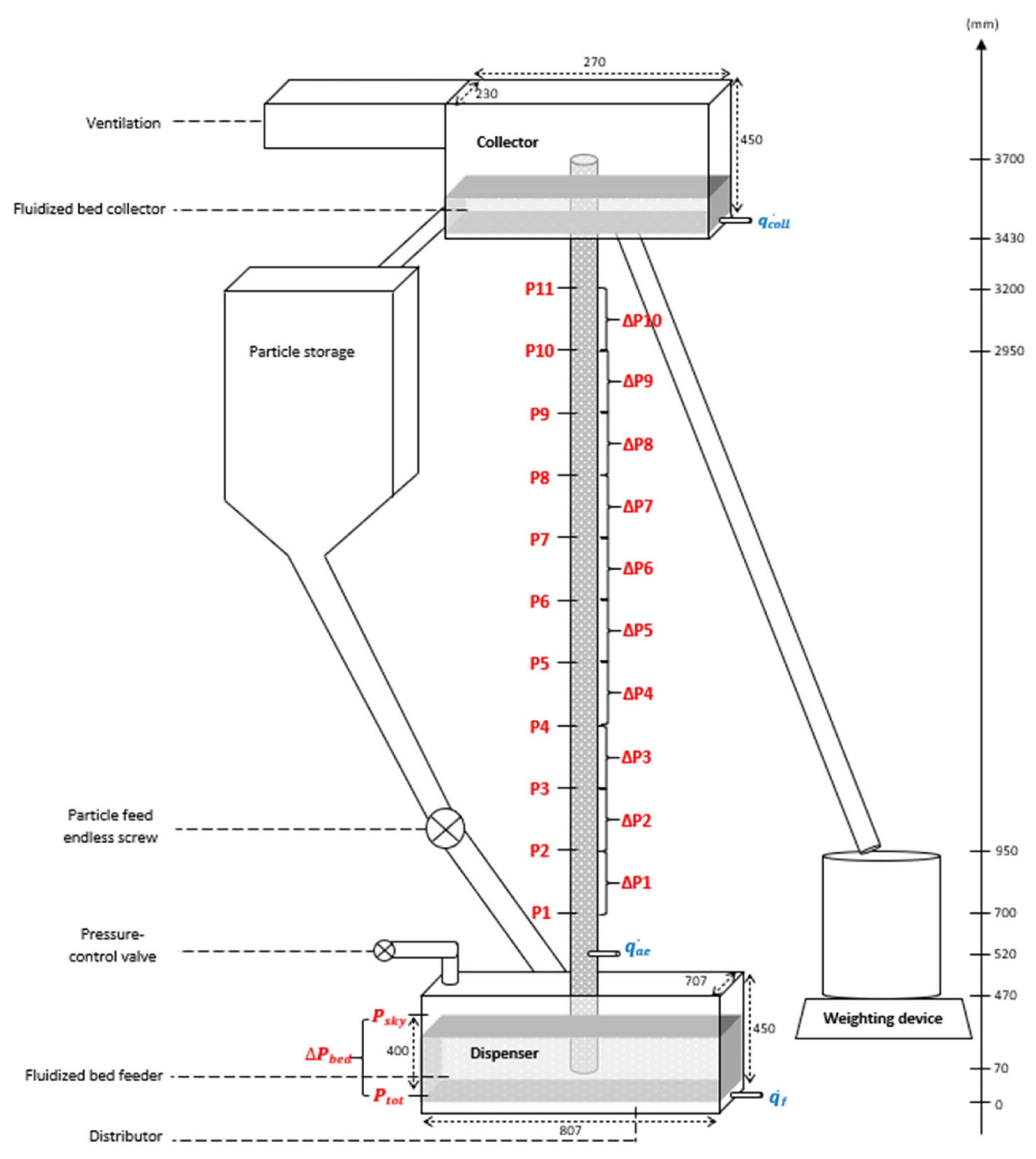
2. Experimental Set-Up
2.1. Cold Mock-Up
- -
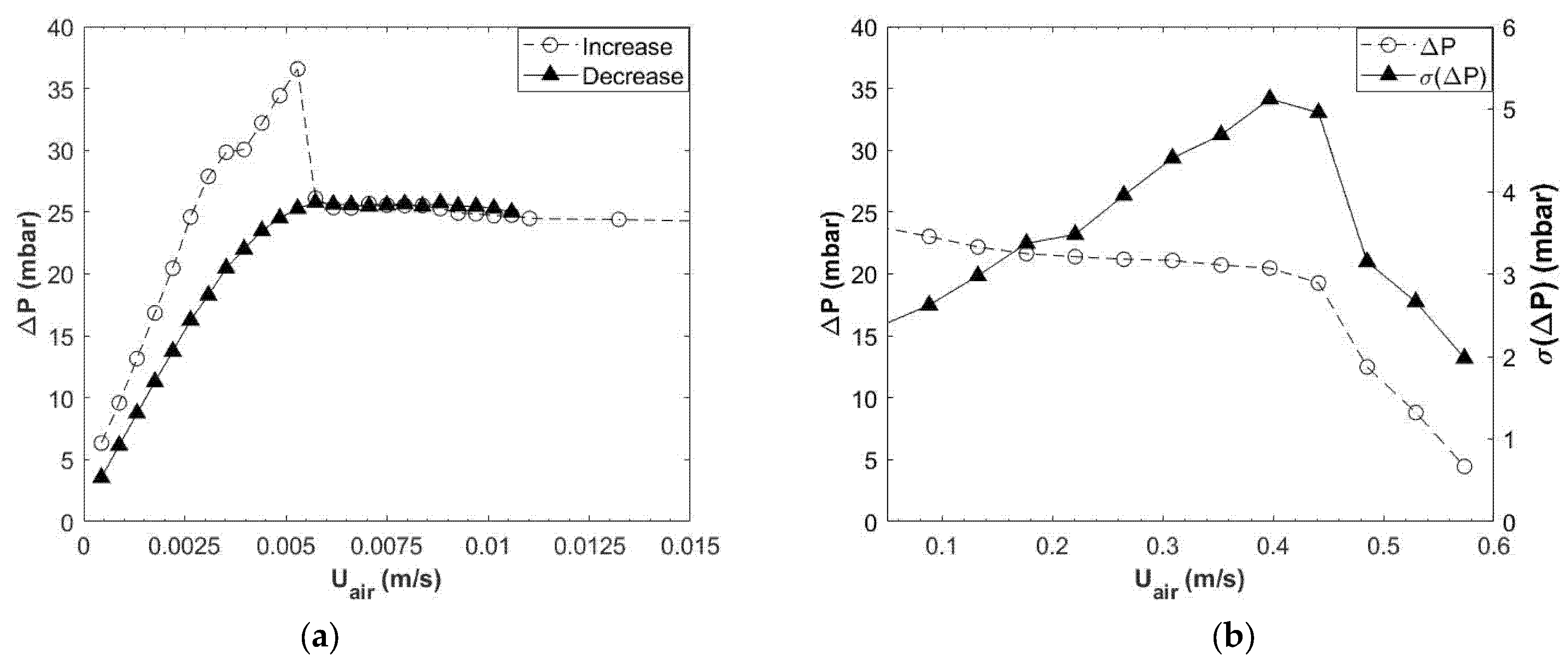
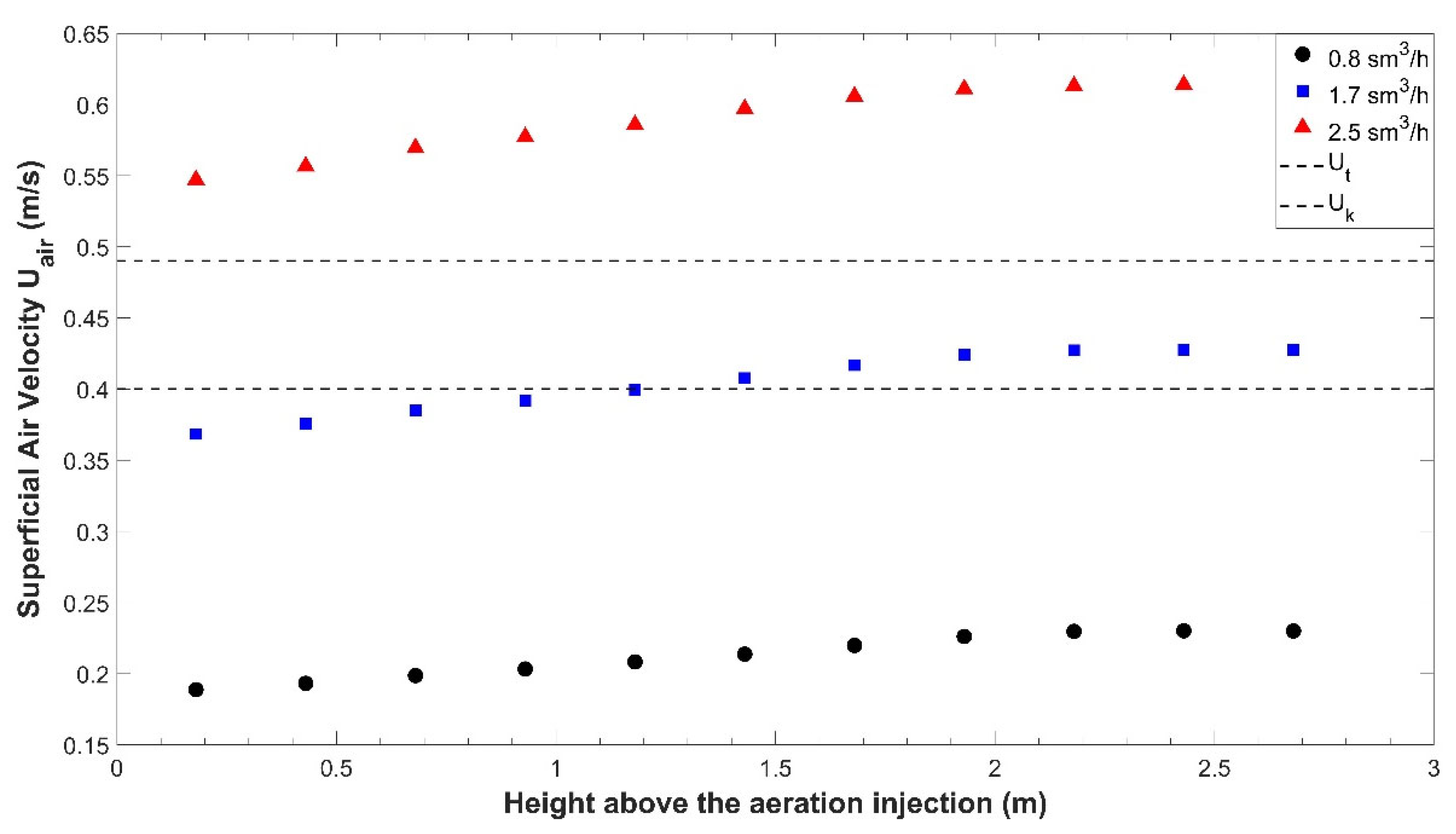
- The aeration air flow rate in the tube ranges from 0.4 to 2.5 sm3/h. The superficial air velocity in the tube is the sum of the superficial velocities in the dispenser and the tube, and respectively, and ranges from 0.01 to 0.54 m/s.
- -
- The driving pressure of the system , i.e., the relative total pressure in the dispenser, varies up to 413 mbar for the tests considered in this paper. Combined with the aeration, it allows the suspension to reach a given height in the tube or to flow at a given mass flow rate outside the tube.
- -
- The level of the suspension in the tube varies but is limited by the tube height 3.18 m above the aeration injection.
- -
- The particles mass flux , i.e., the solid mass flow rate divided by the section of the tube 0.0016 m², is determined by linear regression of the particle mass weight recorded by the weighting scale during an acquisition. It varies during the test campaign up to 122 kg/m²s (698 kg/h).
2.2. Particles
3. Scientific Background
3.1. Solid Volume Fraction Analysis
- -
- A pressure drop due to the energy used to accelerate the particles until the particle velocity, .
- -
- A pressure drop due to the effective weight of the suspension, .
- -
- A pressure drop due to the friction against the tube walls, , with the friction coefficient calculated at 0.925 by the method described by [31].
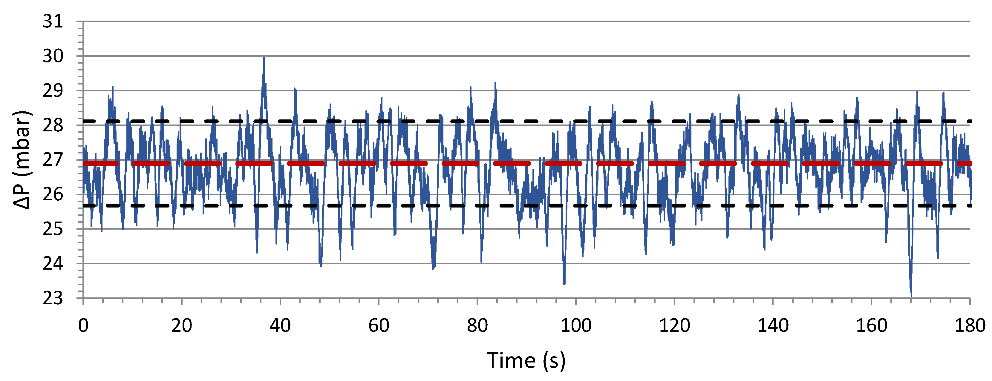
3.2. Temporal Analyses
3.2.1. The Cross-Correlation
3.2.2. The Coherence Analysis
4. Results
4.1. Experimental Parameters of the Compared Acquisitions
4.2. Identification of the Fluidization Regimes in the Tube
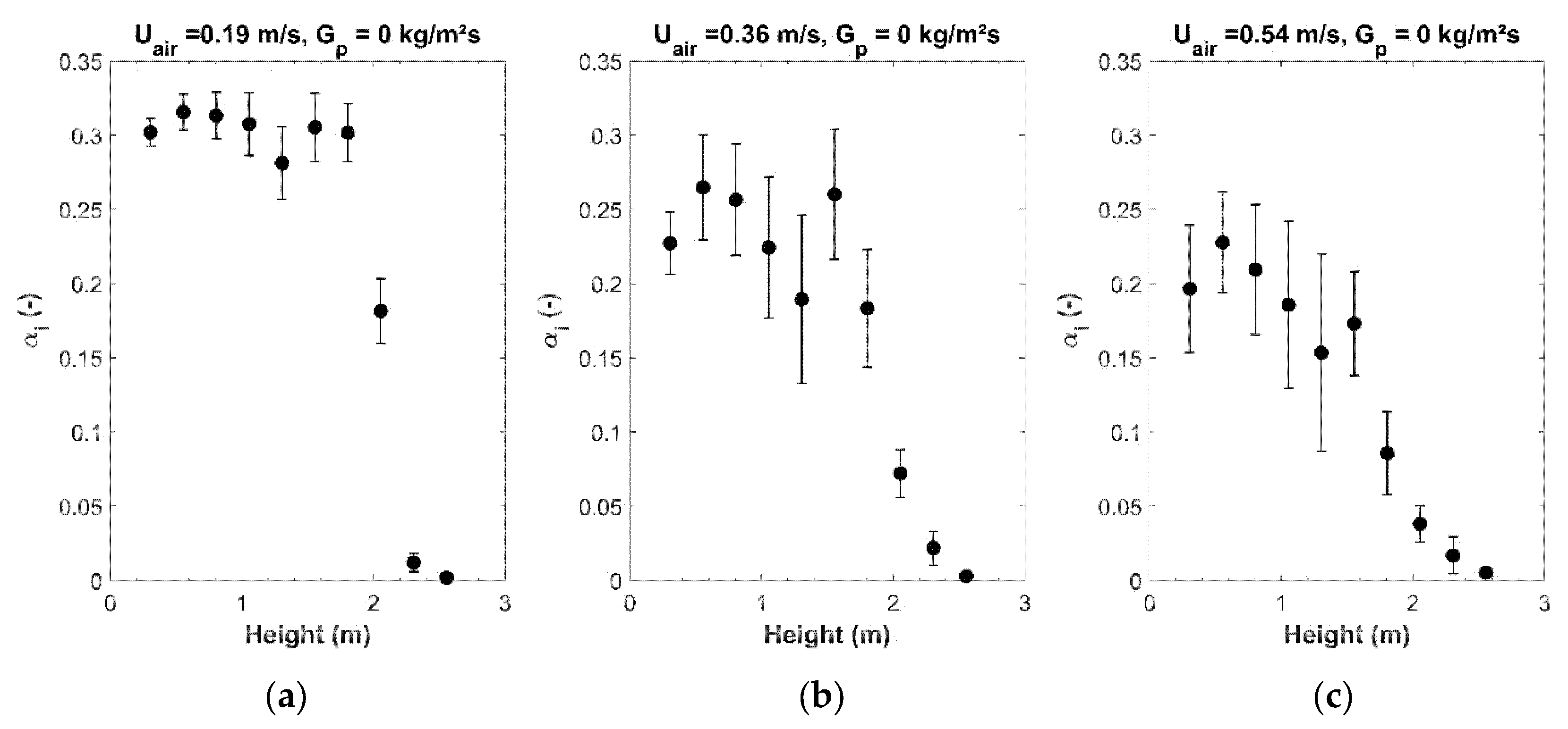
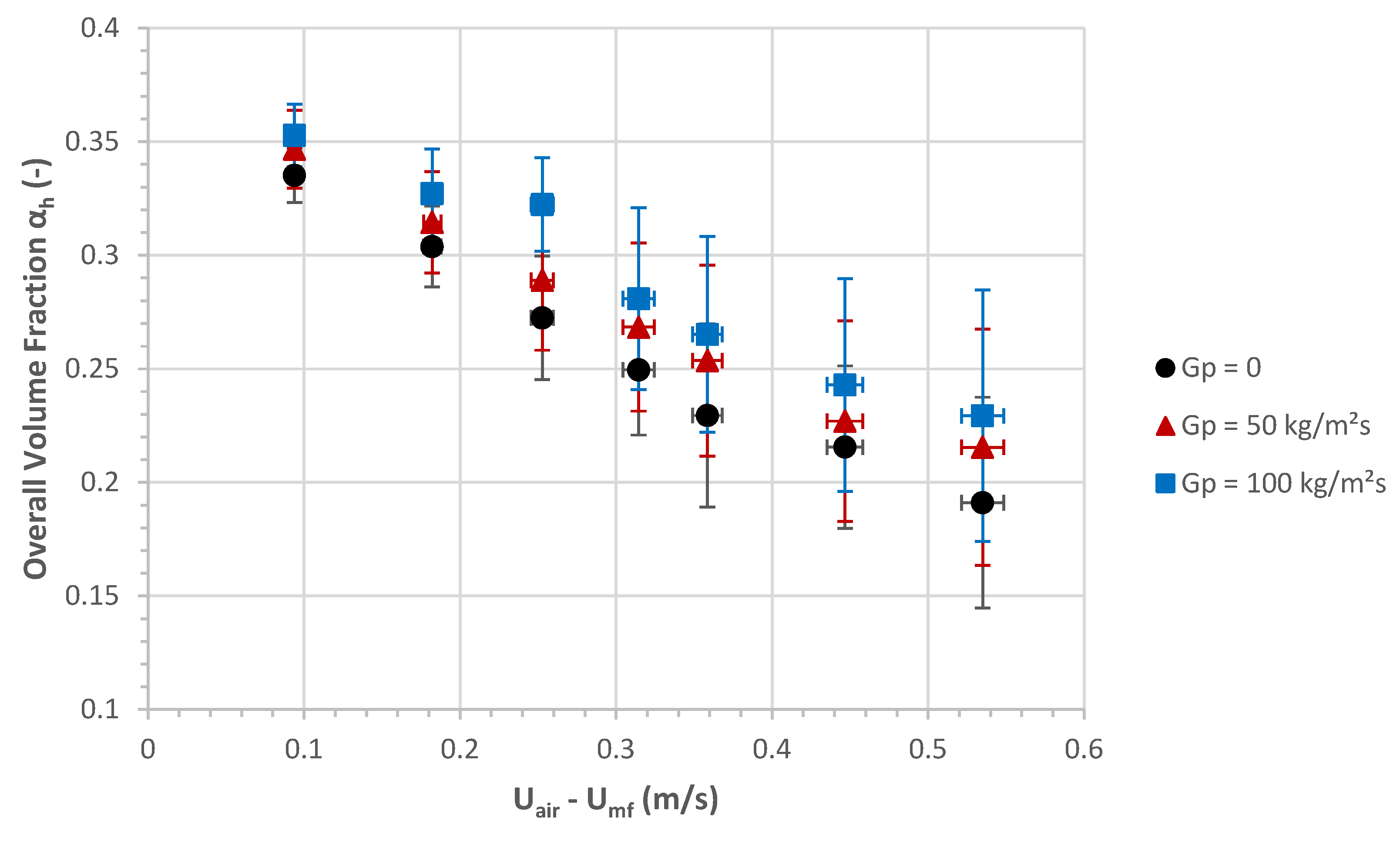
4.2.1. Solid Volume Fraction
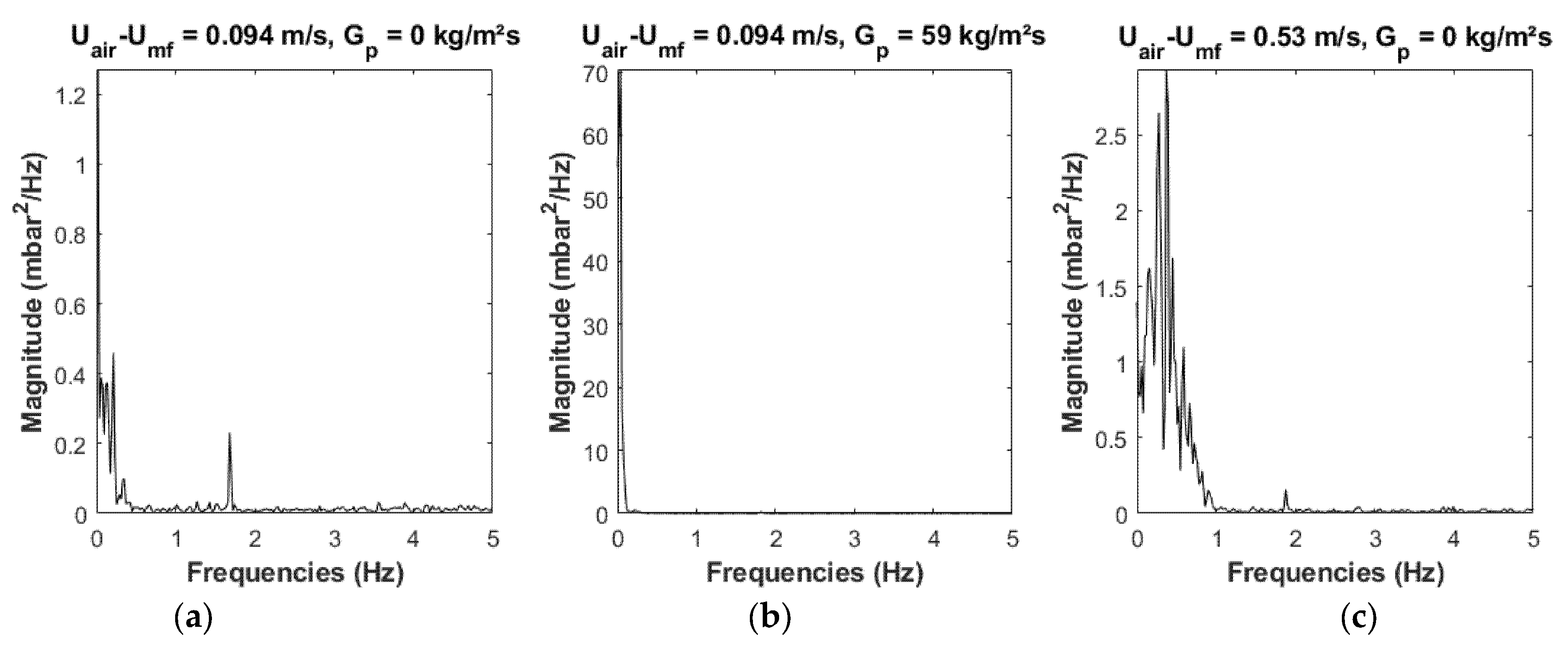
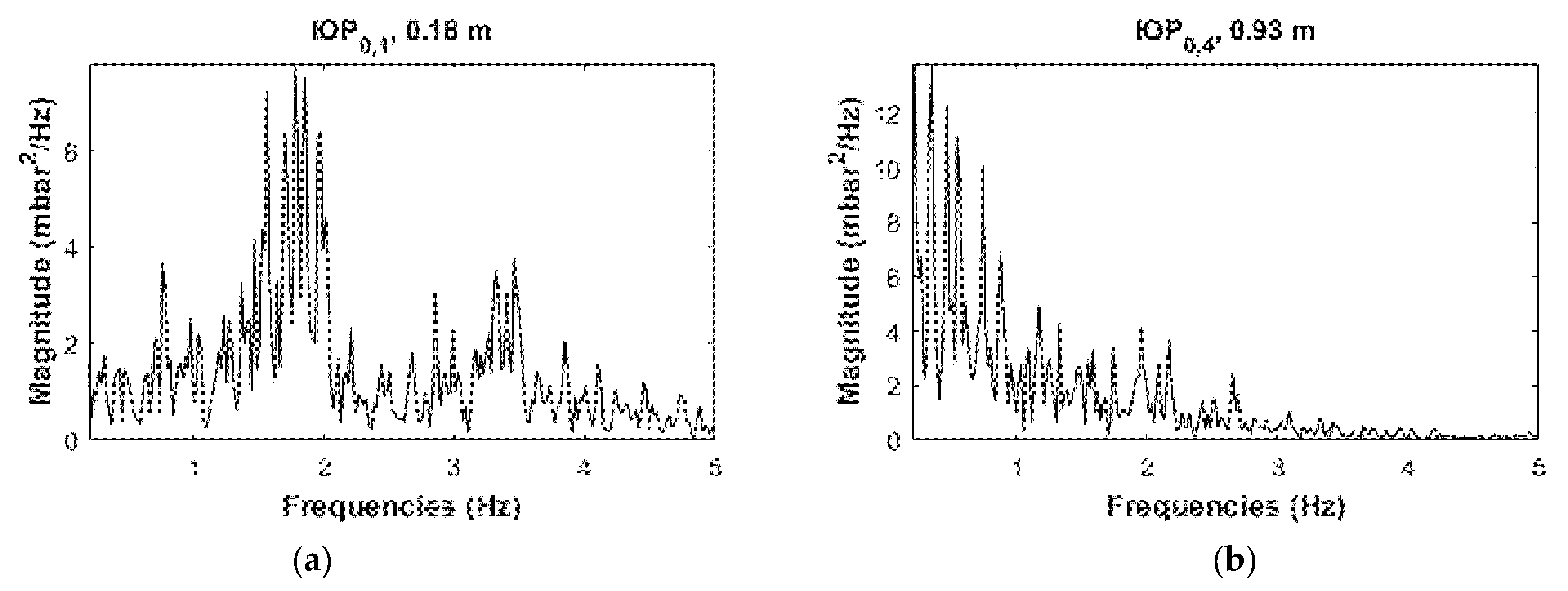
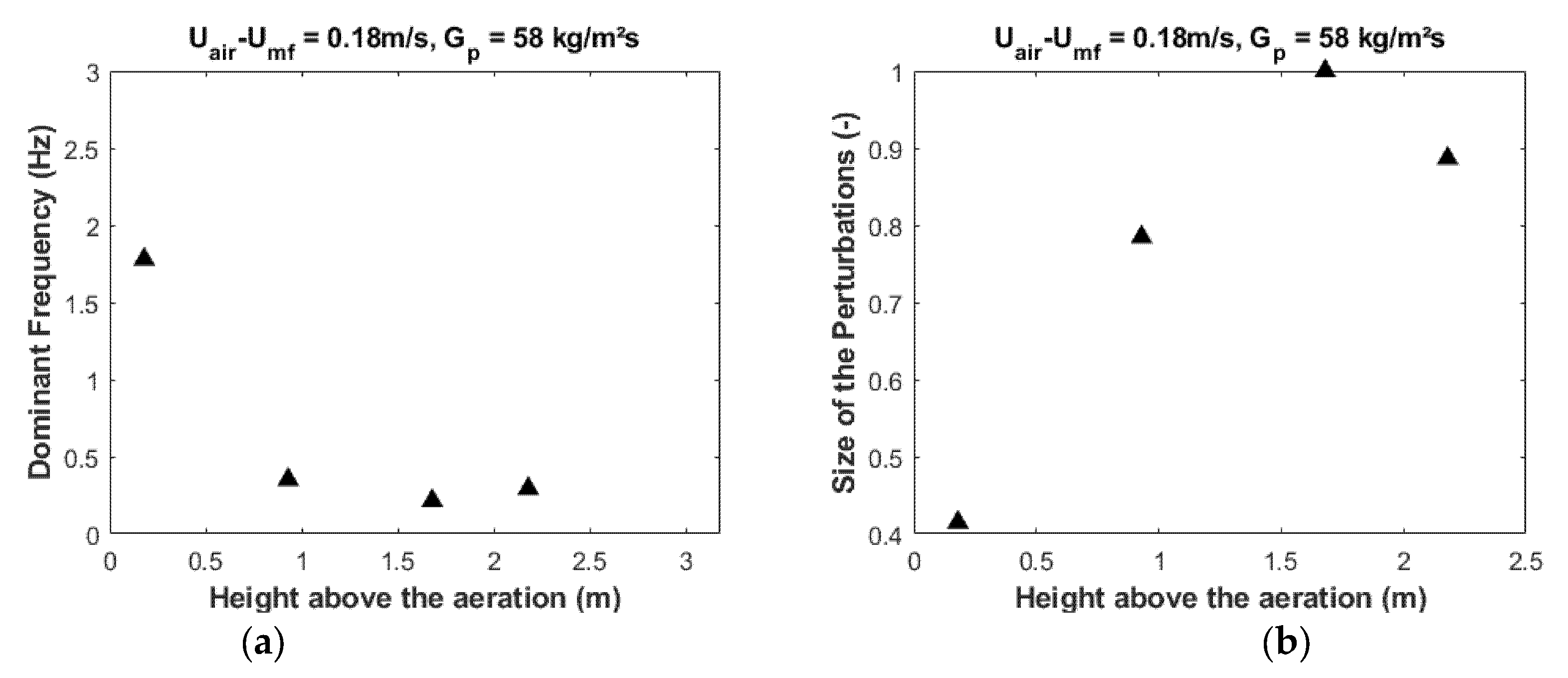
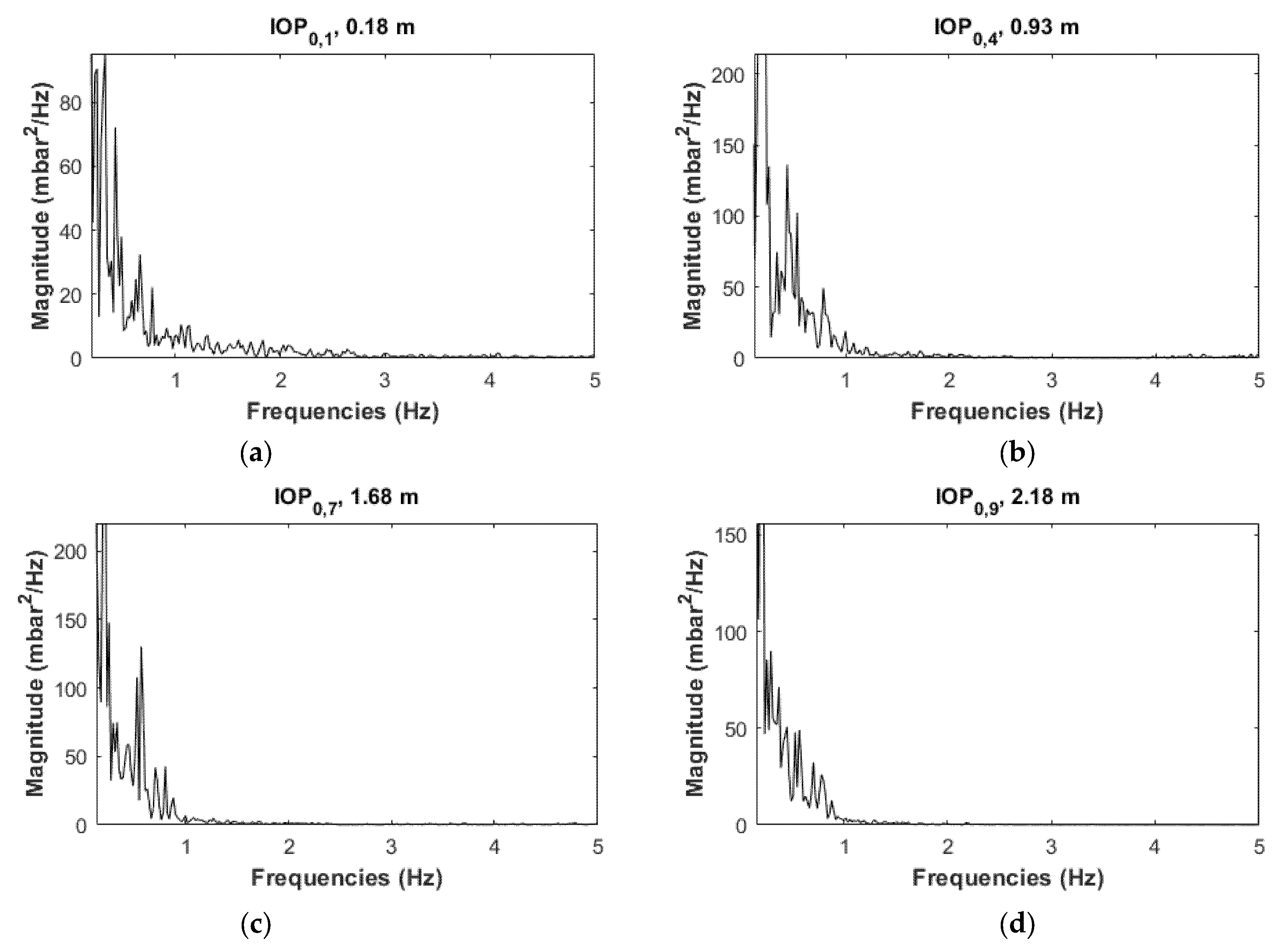
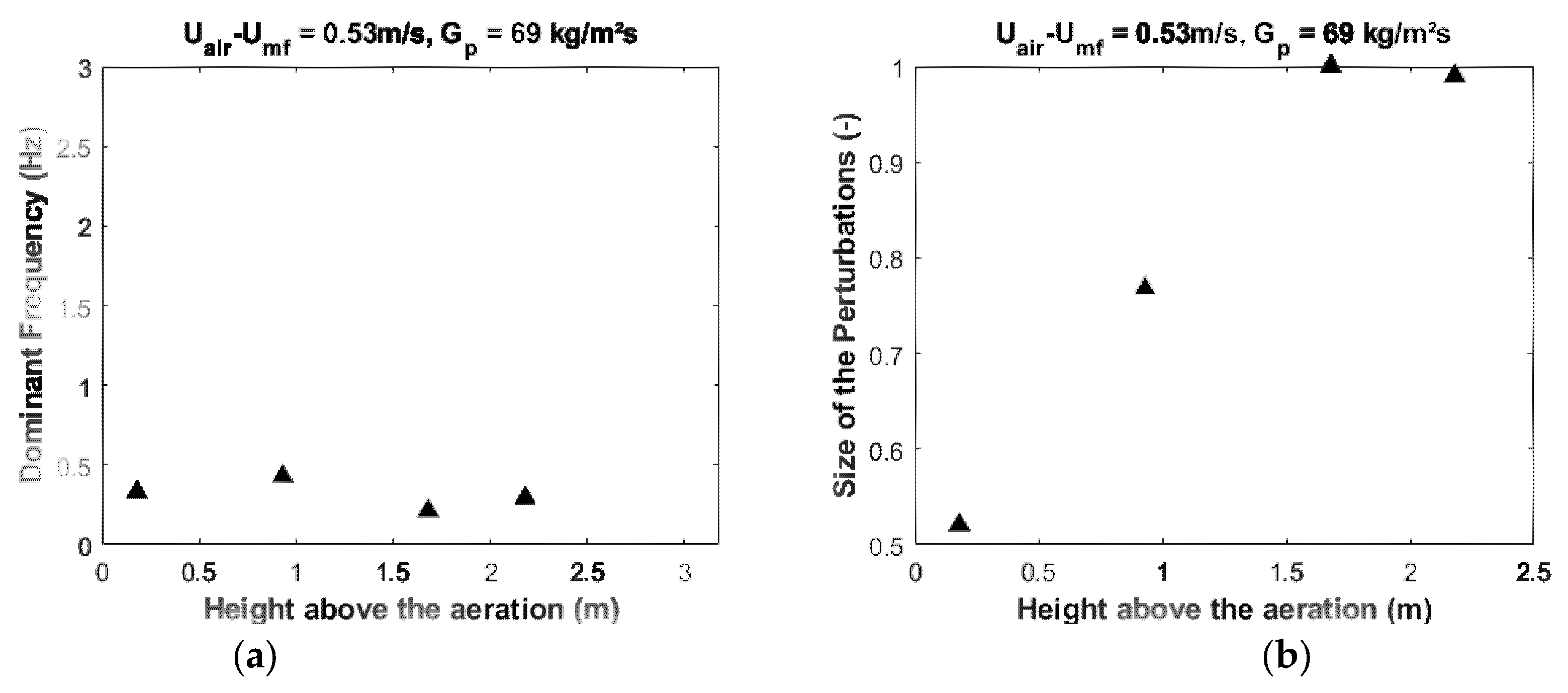
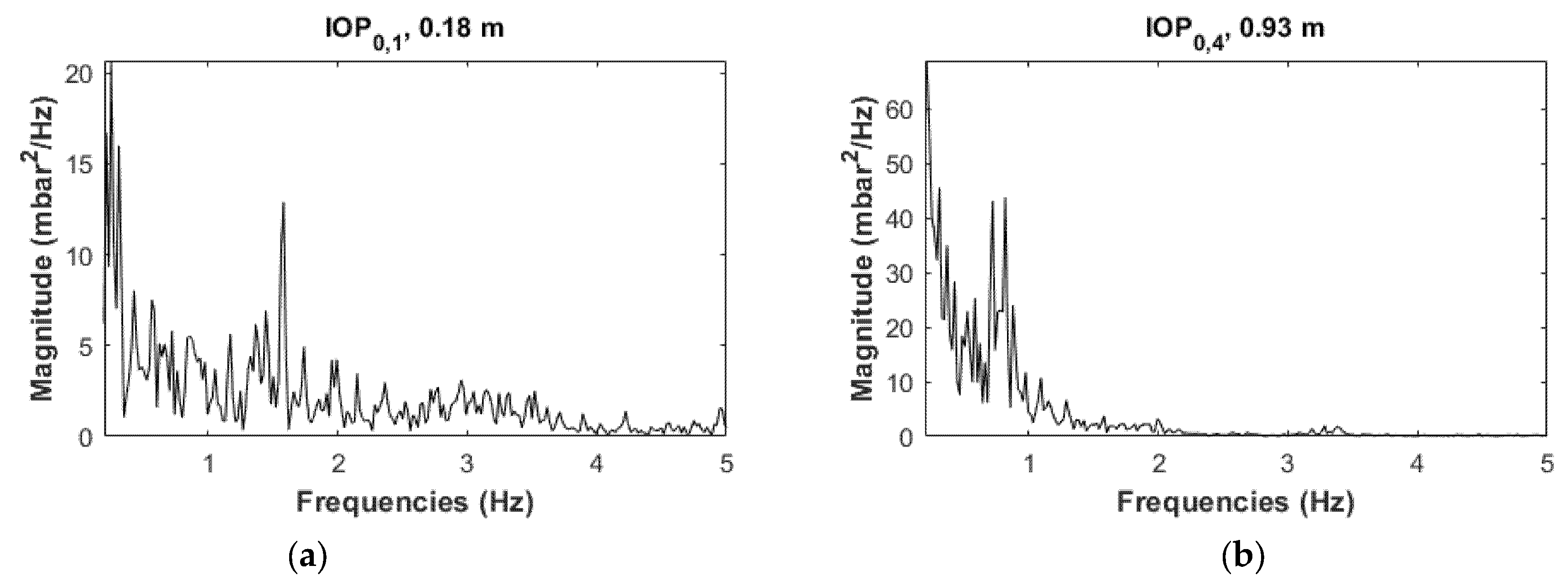
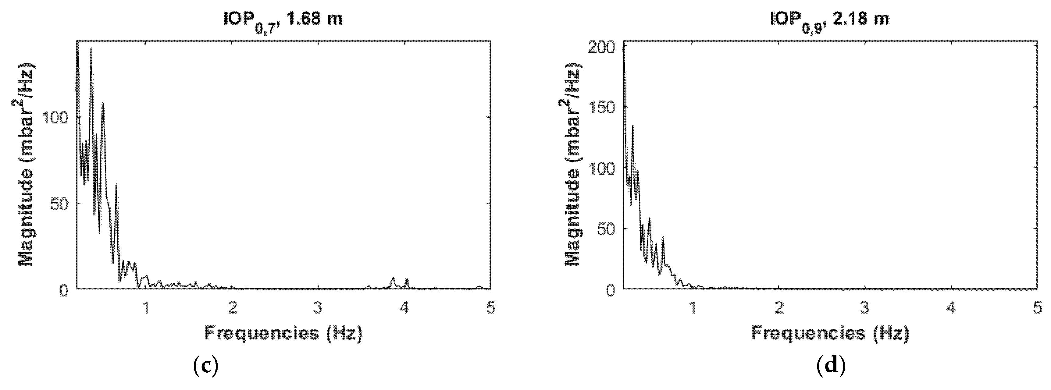
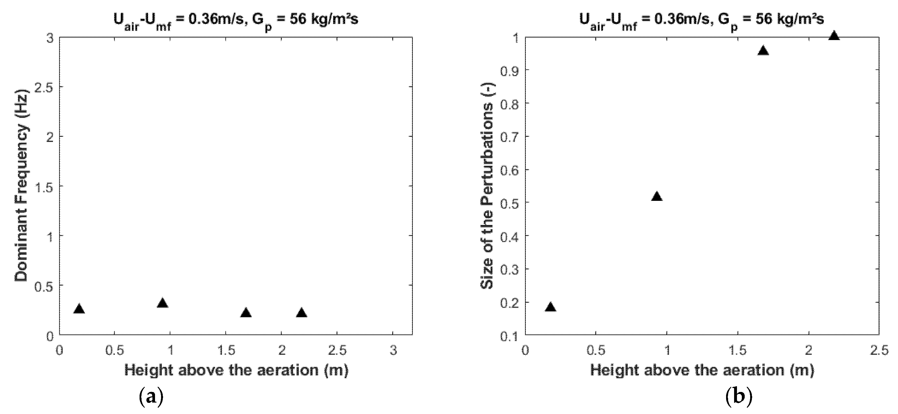
4.2.2. Power Spectrum Analyses
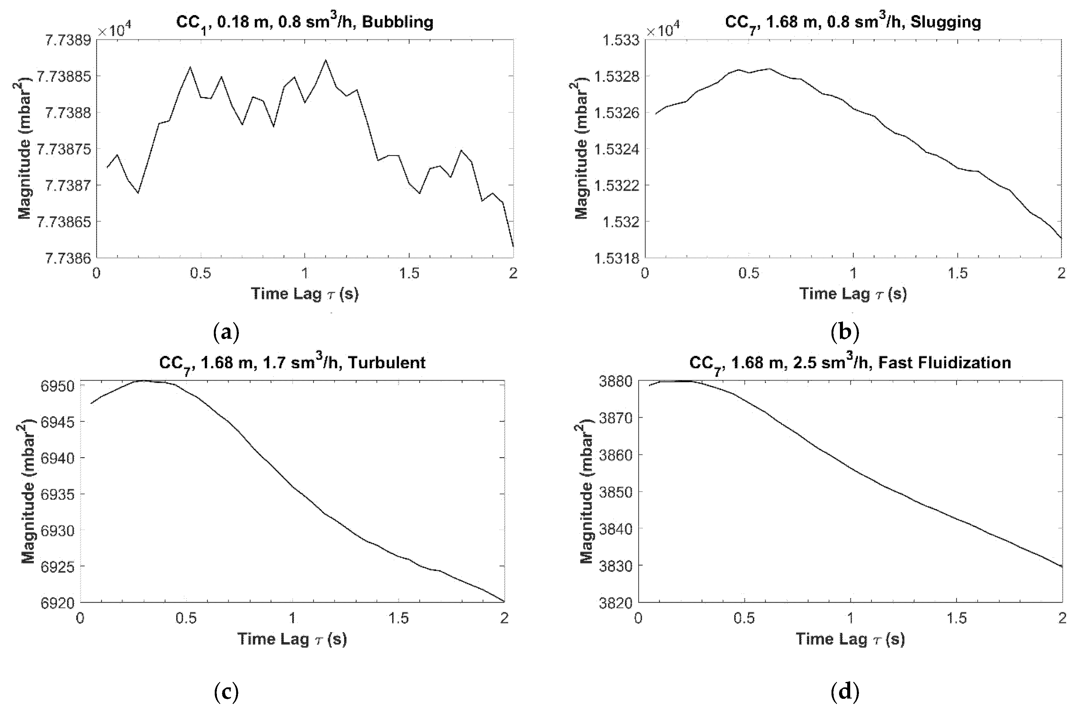
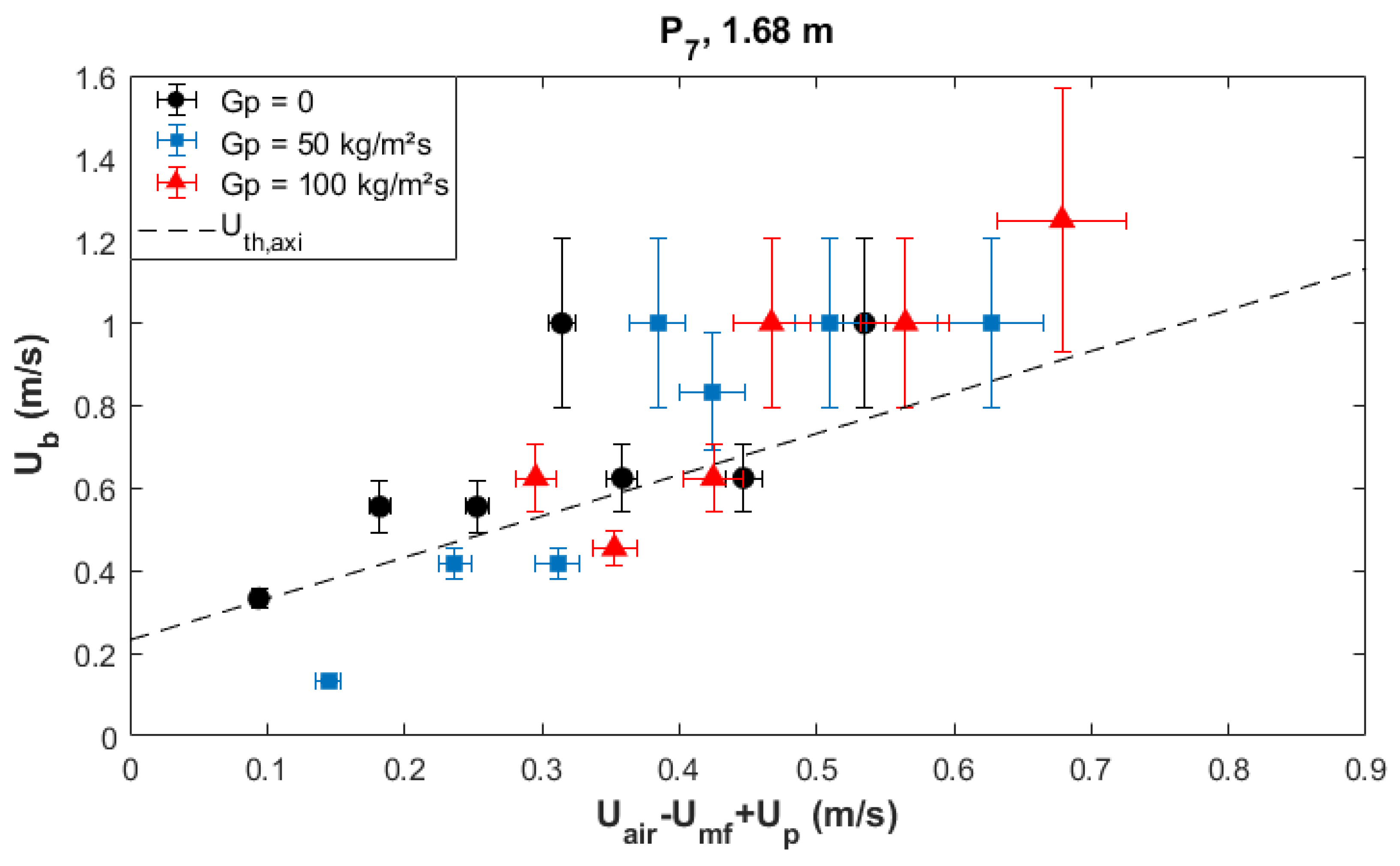
4.2.3. Cross-Correlation Analyses
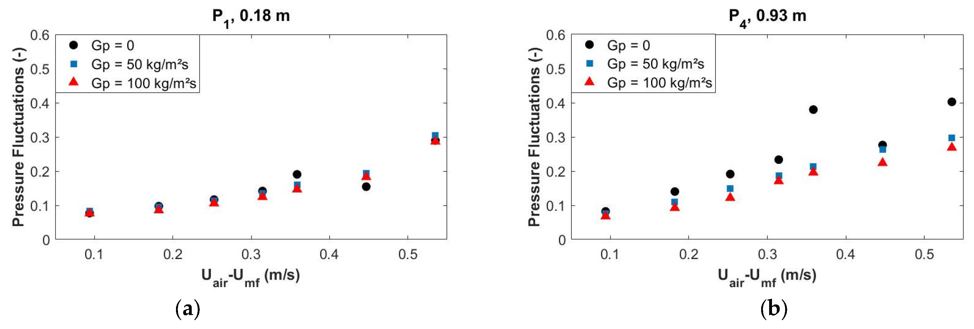
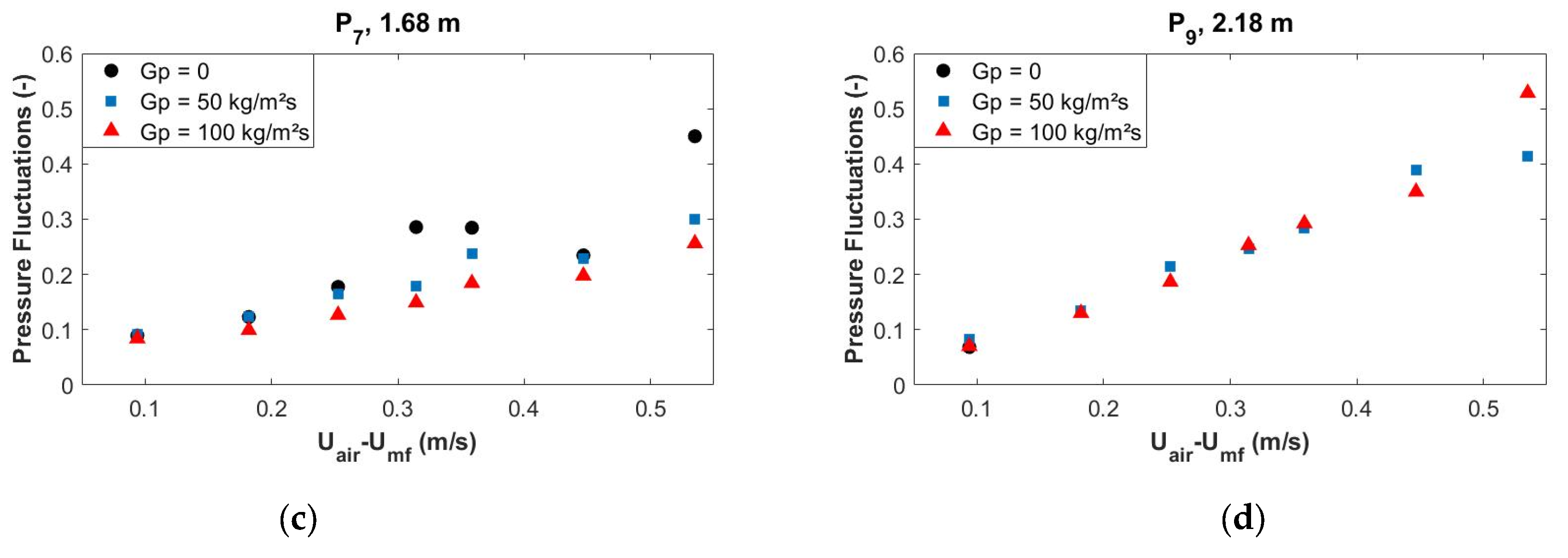
4.2.4. Pressure Fluctuations Amplitude
4.3. Synthesis
5. Conclusions
Author Contributions
Funding
Institutional Review Board Statement
Informed Consent Statement
Data Availability Statement
Acknowledgments
Conflicts of Interest
Nomenclature
| Archimedes number (-) | |
| Friction coefficient (-) | |
| Sauter diameter of the olivine sample (μm) | |
| Volume diameter of the olivine sample (μm) | |
| Diameter corresponding to the X% value on the cumulated particle size distribution | |
| Internal diameter of the glass tube (m) | |
| Acquisition frequency (Hz) | |
| Fourier transform of the signal | |
| Standard acceleration due to gravity (m/s²) | |
| Particle mass flux (kg/m²s) | |
| Height of the suspension inside the tube (m) | |
| Height of the glass tube (m) | |
| Incoherent part of the ith pressure signal | |
| Particle mass flow rate (kg/h) | |
| Number of groups of points each used in the PSD calculation | |
| Number of points recorded in an acquisition | |
| Total relative pressure of the dispenser (mbar) | |
| Relative pressure in the tube at the level of a pressure probe (mbar) | |
| Aeration air flow rate in the tube (sm3/h) | |
| Fluidization air flow rate through the dispenser (sm3/h) | |
| . | Cross-correlation function between the Pi and pressure signals |
| Section of the dispenser (m²) | |
| Section of the tube (m²) | |
| Superficial aeration air velocity in the tube, due to (m/s) | |
| Superficial total air velocity in the tube, (m/s) | |
| Superficial air velocity in the dispenser, due to (m/s) | |
| Upward slug velocity (m/s) | |
| Upward slug velocity, calculated with the two-phases theory (m/s) | |
| Slip velocity between the air and the particles (m/s) | |
| Upward void velocity, determined by the cross-correlation method (m/s) | |
| Minimum bubbling velocity (m/s) | |
| Minimum fluidization velocity (m/s) | |
| Fast fluidization velocity (m/s) | |
| Upward particle velocity (m/s) | |
| Turbulent velocity (m/s) | |
| Local solid volume fraction in the tube, measured between two pressure sockets (-) | |
| Overall solid volume fraction in the tube (-) | |
| Particle volume fraction (-) | |
| Coherence between the ith pressure signal and the “0” reference (-) | |
| Distance between two sockets in the tube (m) | |
| Pressure drop due to the acceleration of the particles (mbar) | |
| Pressure drop due to the friction against the tube walls (mbar) | |
| Differential pressure in the tube between two pressure sockets (mbar) | |
| Pressure drop due to the effective weight of the suspension (mbar) | |
| Porosity (-) | |
| Density of the air (kg/m3) | |
| Bulk density of the olivine (kg/m3) | |
| Spread of the olivine sample (-) | |
| Standard deviation of the pressure signal (mbar) | |
| Mean sphericity of the olivine sample (-) | |
| Cross Power Spectral Density between the ith pressure signal and the “0” reference | |
| Power Spectral Density of the ith pressure signal | |
| Time lag of the cross-correlation function (s) |
Appendix A. Instrumentation of the Mock-Up

| Device | Brand | Model | Measurement Range | Use | |
|---|---|---|---|---|---|
| Relative Pressure Sensors | Keller | PR33X | 0–500 mbar | 8 Hz | |
| Siemens | 7MF1641 | 0–600 mbar | 5 ms | P1–P11 | |
| Differential Pressure Sensors | Rosemont | 2051C | 0–50 mbar | 0.6 Hz | |
| Flowmeters | Brooks | 5853E | 0–2.5 sm3/h | ||
| Brooks | 5853S | 0–16.8 sm3/h | |||
| Acquisition Systems | GraphTec | Midi Logger GL840 | 20 Inputs | 1 Hz | |
| National Instruments | USB-6218 | 16 Inputs | 15,625 kHz |
References
- Benoit, H.; Spreafico, L.; Gauthier, D.; Flamant, G. Review of heat transfer fluids in tube-receivers used in concentrating solar thermal systems: Properties and heat transfer coefficients. Renew. Sustain. Energy Rev. 2016, 55, 298–315. [Google Scholar] [CrossRef]
- Zhang, H.; Kong, W.; Tan, T.; Baeyens, J. High-efficiency concentrated solar power plants need appropriate materials for high-temperature heat capture, conveying and storage. Energy 2017, 139, 52–64. [Google Scholar] [CrossRef]
- Ho, C.K.; Christian, J.; Yellowhair, J.; Jeter, S.; Golob, M.; Nguyen, C.; Repole, K.; Abdel-Khalik, S.; Siegel, N.; Al-Ansary, H.; et al. Highlights of the high-temperature falling particle receiver project: 2012–2016. AIP Conf. Proc. 2017, 1850, 030027. [Google Scholar] [CrossRef] [Green Version]
- Wu, W.; Amsbeck, L.; Buck, R.; Uhlig, R.; Ritz-Paal, R. Proof of concept test of a centrifugal particle receiver. Energy Procedia 2014, 49, 560–568. [Google Scholar] [CrossRef] [Green Version]
- Flamant, G.; Hemati, H. Dispositif Collecteur D’énergie Solaire (Device for Collecting Solar Energy). French Patent FR 1058565, 20 October 2010. PCT Extension WO2012052661, 26 April 2012. [Google Scholar]
- Gueguen, R.; Grange, B.; Bataille, F.; Mer, S.; Flamant, G. Shaping High Efficiency, High Temperature Cavity Tubular Solar Receivers. Energies 2020, 13, 4803. [Google Scholar] [CrossRef]
- Behar, O.; Grange, B.; Flamant, G. Design and performance of a modular combined cycle solar power plant using the fluidized particle solar receiver technology. Energy Convers. Manag. 2020, 220, 113108. [Google Scholar] [CrossRef]
- Jacob, R.; Belusko, M.; Ines Fernandez, A.; Cabeza, L.F.; Saman, W.; Bruno, F. Embodied energy and cost of high temperature thermal energy storage systems for use with concentrated solar power plants. Appl. Energy 2016, 180, 586–597. [Google Scholar] [CrossRef] [Green Version]
- Kang, Q.; Flamant, G.; Dewil, R.; Baeyens, J.; Zhang, H.L.; Deng, Y.M. Particles in a circulation loop for solar energy capture and storage. Particuology 2019, 43, 149–156. [Google Scholar] [CrossRef]
- CSP2. Dense Suspensions of Solid Particles as a New Heat Transfer Fluid for CSP. Available online: http://www.csp2-project.eu/ (accessed on 10 August 2021).
- Next-CSP. High Temperature Concentrated Solar Thermal Power Plant with Particle Receiver and Direct Thermal Storage. 2020. Available online: http://next-csp.eu/ (accessed on 10 August 2021).
- Benoit, H.; Perez Lopez, I.; Gauthier, D.; Sans, J.-L.; Flamant, G. On-sun demonstration of a 750 °C heat transfer fluid for concentrating solar systems: Dense particle suspension in tube. Sol. Energy 2015, 118, 622–633. [Google Scholar] [CrossRef]
- Le Gal, A.; Grange, B.; Tessonneaud, M.; Perez, A.; Escape, C.; Sans, J.-L.; Flamant, G. Thermal analysis of fluidized particle flows in a finned tube solar receiver. Sol. Energy 2019, 191, 19–33. [Google Scholar] [CrossRef]
- Perez-Lopez, I.; Benoit, H.; Gauthier, D.; Sans, J.L.; Guillot, E.; Mazza, G.; Flamant, G. On-sun operation of a 150 kWth pilot solar receiver using dense particle suspension as heat transfer fluid. Sol. Energy 2016, 137, 463–476. [Google Scholar] [CrossRef]
- Boissière, B.; Ansart, R.; Gauthier, D.; Flamant, G.; Hemati, M. Experimental Hydrodynamic Study of Gas-Particle Dense Suspension Upward Flow for Application as New Heat Transfer and Storage Fluid. Can. J. Chem. Eng. 2015, 93, 317–330. [Google Scholar] [CrossRef] [Green Version]
- Sabatier, F.; Ansart, R.; Zhang, H.; Baeyens, J.; Simonin, O. Experiments support simulations by NEPTUNE CFD Code in a Upflow Bubbling Fluidized Bed reactor. Chem. Eng. J. 2020, 385, 123568. [Google Scholar] [CrossRef]
- Deng, Y.; Sabatier, F.; Dewil, R.; Flamant, G.; Le Gal, A.; Gueguen, R.; Baeyens, J.; Li, S.; Ansart, R. Dense upflow fluidized bed (DUFB) solar receivers of high aspect ratio: Different fluidization modes through inserting bubble rupture promoters. Chem. Eng. J. 2021, 418, 129376. [Google Scholar] [CrossRef]
- Geldart, D. Chap. 2: Single particles, Fixed and Quiescent Beds. In Gas Fluidization Technology; John Wiley & Sons Ltd.: Chichester, UK, 1986; pp. 11–32. [Google Scholar]
- Kong, W.; Tan, T.; Baeyens, J.; Flamant, G.; Zhang, H. Bubbling and slugging of Geldart group A powders in small diameters columns. Ind. Eng. Chem. Res. 2017, 56, 4136–4144. [Google Scholar] [CrossRef]
- Grace, J.R.; Bi, X.; Ellis, N. Chap. 9: Turbulent Fluidization. In Essential of Fluidization Technology; John Wiley & Sons Ltd.: Chichester, UK, 2020; pp. 163–180. [Google Scholar]
- Dodds, J.; Baluais, G. Particle size characterization. Sci. Géologiques 1993, 46, 79–104. [Google Scholar]
- Geldart, D. Types of Gas Fluidization. Powder Technol. 1973, 7, 285–292. [Google Scholar] [CrossRef]
- Davidson, J.F.; Harrison, D. Chap. 2: Incipient fluidization and particulate systems. In Fluidization; Academic Press: Cambridge, MA, USA, 1971. [Google Scholar]
- Wu, S.Y.; Baeyens, J. Effect of operating temperature on minimum fluidization velocity. Powder Technol. 1991, 67, 217–220. [Google Scholar]
- Kunii, D.; Levenspiel, O. Chap. 3: Fluidization and Mapping of Regimes. In Fluidization Engineering, 2nd ed.; Butterworth-Heinemann: Newton, MA, 1991; pp. 61–94. [Google Scholar]
- Abrahamsen, A.R.; Geldart, D. Behaviour of Gas-Fluidized Beds of Fine Powders Part I. Homogeneous Expansion. Powder Technol. 1980, 26, 35–46. [Google Scholar] [CrossRef]
- Grace, J.R.; Bi, X.; Ellis, N. Chap. 4: Gas Fluidization Flow Regimes. In Essential of Fluidization Technology; John Wiley & Sons Ltd.: Chichester, UK, 2020; pp. 55–74. [Google Scholar]
- Bi, H.T.; Ellis, N.; Abba, I.A.; Grace, J.R. A state-of-the-art review of gas-solid turbulent fluidization. Chem. Eng. Sci. 2000, 55, 4789–4825. [Google Scholar] [CrossRef]
- Rabinovich, E.; Kalman, H. Flow regime diagram for vertical pneumatic conveying and fluidized bed systems. Powder Technol. 2011, 207, 119–133. [Google Scholar] [CrossRef]
- Zhang, H.; Kong, W.; Tan, T.; Flamant, G.; Baeyens, J. Experiments support an improved model for particle transport in fluidized beds. Sci. Rep. 2017, 7, 10178. [Google Scholar] [CrossRef]
- Geldart, D. Chap. 6: Particle Entrainment and Carryover. In Gas Fluidization Technology; John Wiley & Sons Ltd.: Chichester, UK, 1986; pp. 123–154. [Google Scholar]
- Srivastava, A.; Sundaresan, S. Role of wall friction in fluidization and standpipe flow. Powder Technol. 2002, 124, 45–54. [Google Scholar] [CrossRef]
- Geldart, D. Chap. 4: Hydrodynamics of Bubbling Fluidized Beds. In Gas Fluidization Technology; John Wiley & Sons Ltd.: Chichester, UK, 1986; pp. 53–96. [Google Scholar]
- Puncochar, M.; Drahos, J. Origin of pressure fluctuations in fluidized beds. Chem. Eng. Sci. 2005, 60, 1193–1197. [Google Scholar] [CrossRef]
- Bi, H. A critical review of the complex pressure fluctuation phenomenon in gas-solids fluidized beds. Chem. Eng. Sci. 2007, 62, 3473–3493. [Google Scholar] [CrossRef]
- Johnsson, F.; Zijerveld, R.C.; Schouten, J.C.; van den Bleek, C.M.; Leckner, B. Characterization of fluidization regimes by time-series analysis of pressure fluctuations. Int. J. Multiph. Flow 2000, 26, 663–715. [Google Scholar] [CrossRef]
- Fan, L.T.; Ho, T.C.; Walawender, W.P. Measurements of the Rise Velocities of Bubbles, Slugs and Pressure Waves in a Gas-Solid Fluidized Bed Using Pressure Fluctuation Signals. AIChE J. 1983, 29, 33–39. [Google Scholar] [CrossRef]
- Van der Schaaf, J.; Schouten, J.C.; Johnsson, F. Non-intrusive determination of bubble and slug length scales in fluidized beds by decomposition of the power spectral density of pressure time series. Int. J. Multiph. Flow 2002, 28, 865–880. [Google Scholar] [CrossRef]
- Grace, J.R.; Bi, X.; Ellis, N. Chap. 8: Slug Flow. In Essential of Fluidization Technology; John Wiley & Sons Ltd.: Chichester, UK, 2020; pp. 153–162. [Google Scholar]
- Plancherel, M.; Leffler, M. Contribution à l’Etude de la Représentation d’une Fonction Arbitraire par des Intégrales Définies. Rend. Circ. Mat. Palermo 1981, 30, 289–335. [Google Scholar]


| (μm) | (μm) | ||||
| Particle size | 61 μm | 81 μm | 75% | 59.6% | 21 |
| (cm/s) | (cm/s) | ( m/s) | (m/s) | ||
| Velocities | 0.42 ± 0.03 | 0.57 ± 0.04 | 0.40 ± 0.04 | 0.49 ± 0.04 |
| 0.4 | 2.40 ± 0.06 m | 59.2 ± 1.7 kg/m²s | 107.1 ± 3.4 kg/m²s |
| 0.8 | 2.08 ± 0.09 m | 58.2 ± 1.6 kg/m²s | 122.0 ± 3.2 kg/m²s |
| 1.2 | 2.30 ± 0.08 m | 56.3 ± 1.4 kg/m²s | 106.6 ± 2.9 kg/m²s |
| 1.5 | 1.86 ± 0.13 m | 62.5 ± 1.8 kg/m²s | 103.3 ± 2.7 kg/m²s |
| 1.7 | 2.03 ± 0.11 m | 56.4 ± 1.5 kg/m²s | 98.9 ± 2.7 kg/m²s |
| 2.1 | 2.08 ± 0.15 m | 52.0 ± 1.3 kg/m²s | 99.2 ± 2.6 kg/m²s |
| 2.5 | 1.88 ± 0.24 m | 69.1 ± 1.7 kg/m²s | 116.8 ± 2.8 kg/m²s |
| Average values | 2.09 ± 0.20 m | 59.1 ± 5.4 kg/m²s | 107.7 ± 8.7 kg/m²s |
Publisher’s Note: MDPI stays neutral with regard to jurisdictional claims in published maps and institutional affiliations. |
© 2021 by the authors. Licensee MDPI, Basel, Switzerland. This article is an open access article distributed under the terms and conditions of the Creative Commons Attribution (CC BY) license (https://creativecommons.org/licenses/by/4.0/).
Share and Cite
Gueguen, R.; Sahuquet, G.; Mer, S.; Toutant, A.; Bataille, F.; Flamant, G. Gas-Solid Flow in a Fluidized-Particle Tubular Solar Receiver: Off-Sun Experimental Flow Regimes Characterization. Energies 2021, 14, 7392. https://doi.org/10.3390/en14217392
Gueguen R, Sahuquet G, Mer S, Toutant A, Bataille F, Flamant G. Gas-Solid Flow in a Fluidized-Particle Tubular Solar Receiver: Off-Sun Experimental Flow Regimes Characterization. Energies. 2021; 14(21):7392. https://doi.org/10.3390/en14217392
Chicago/Turabian StyleGueguen, Ronny, Guillaume Sahuquet, Samuel Mer, Adrien Toutant, Françoise Bataille, and Gilles Flamant. 2021. "Gas-Solid Flow in a Fluidized-Particle Tubular Solar Receiver: Off-Sun Experimental Flow Regimes Characterization" Energies 14, no. 21: 7392. https://doi.org/10.3390/en14217392