
A Fast and Improved Tunable Aggregation Model for Stochastic Simulation of Spray Fluidized Bed Agglomeration


Thermal Process Engineering, Faculty of Process and Systems Engineering, Otto von Guericke University, Universitätsplatz 2, 39106 Magdeburg, Germany
*
Author to whom correspondence should be addressed.
Energies 2021, 14(21), 7221; https://doi.org/10.3390/en14217221
Submission received: 8 October 2021
/
Revised: 26 October 2021
/
Accepted: 28 October 2021
/
Published: 2 November 2021
(This article belongs to the Special Issue Progress and Novel Applications of Fluidized Bed Technology)
Abstract
:Agglomeration in spray fluidized bed (SFB) is a particle growth process that improves powder properties in the chemical, pharmaceutical, and food industries. In order to analyze the underlying mechanisms behind the generation of SFB agglomerates, modeling of the growth process is essential. Morphology plays an imperative role in understanding product behavior. In the present work, the sequential tunable algorithm developed in previous studies to generate monodisperse SFB agglomerates is improved and extended to polydisperse primary particles. The improved algorithm can completely retain the given input fractal properties (fractal dimension and prefactor) for polydisperse agglomerates (with normally distributed radii of primary particles having a standard deviation of 10% from the mean value). Other morphological properties strongly agreed with the experimental SFB agglomerates. Furthermore, this tunable aggregation model is integrated into the Monte Carlo (MC) simulation. The kinetics of the overall agglomeration at various operating conditions, like binder concentration and inlet fluidized gas temperature, are investigated. The present model accurately predicts the morphological descriptors of SFB agglomerates and the overall kinetics under various operating parameters.
1. Introduction
The comprehensive morphological characterization of agglomerates is becoming increasingly important in the chemical, food, and pharmaceutical industries, as well as in research. This is due to the dependence of functional properties on the microscopic structure leading to different macroscopic features, like density, flowability, and strength [1]. Therefore, techniques to produce particles that allow control of the agglomerate morphology are highly desirable. In this regard, agglomeration in a spray fluidized bed (SFB) is a particle growth process that enhances the physical properties of small particles [2]. In this process, particles are fluidized through the air, also used as a drying agent. The surface of the fluidized particles is wetted by binder droplets sprayed through a nozzle. After successful collisions of the fluidized particles with each other, liquid bridges are formed. Water contained in the liquid bridges evaporates and leads to the formation of solid bonds between the primary particles in an agglomerate. The morphology of formed agglomerates is similar to that of a blackberry [3].
In order to understand and analyze the mechanisms behind the generation of porous particles bigger than the original particles, modeling of the growth process is crucial. Macroscopically, population balance equations are commonly used [4,5], and microscopically, Monte Carlo (MC) models [6,7,8,9,10] and discrete element methods coupled with or without computational fluid dynamics [11,12,13,14,15] are used. The focus of the present work is on the modeling of SFB agglomeration operated in batch mode. In this work, the overall SFB agglomeration, consisting of several micro-scale mechanisms, is simulated using the MC method. This method is employed to describe random mechanisms on a microscale, by creating a scaled-down virtual SFB granulator. This approach is similar to the technique used by Terrazas et al. [16], Dernedde et al. [7], and Singh and Tsotsas [9,10].
Morphological analysis of the agglomerates is necessary to capture the temporal growth of particles during agglomeration. It plays a crucial role in evaluating the various underlying mechanisms on a microscale behind the agglomeration process. Agglomerates are polymorphic and are characterized using fractal properties such as prefactor and fractal dimension, porosity, and coordination number. An increasing interest in investigating the morphology of aggregates has stimulated the exploration for numerical algorithms that could provide results similar to experimental findings. From the plethora of aggregation algorithms in the literature, the particle–cluster tunable aggregation model predicts SFB agglomerates quite well. An overview of the tunable aggregation model developed over the years is given in [10]. The first tunable aggregation algorithm was introduced by [17]. Subsequently, several other studies have proposed different tunable algorithms to generate aggregates. However, only the fractal dimension was preserved in most of these studies [18,19,20]. In order to determine the morphology of an agglomerate, both fractal dimension and prefactor must be correctly ascertained [21,22].
A notable exception is an algorithm proposed by Filippov et al. [23], which could preserve both fractal dimension and prefactor. This algorithm was further extended and adapted in various fields to investigate the morphology of fractal aggregates [10,24,25,26,27,28]. Relatively compact SFB agglomerates were observed in the experiments [29]. However, these SFB agglomerates with a combination of large prefactor , with large fractal dimension (cf. Table A1) cannot be reconstructed using the original versions of the algorithms presented in the past. This is due to the limitation of the prefactor at higher fractal dimension. Singh and Tsotsas [10] developed a tunable sequential aggregation (TSA) algorithm to reconstruct the SFB agglomerate corresponding to its fractal properties. The TSA model reconstructed SFB agglomerates that are composed of monodisperse primary particles by tuning their fractal properties [10]. Regardless of each agglomerate having a variable fractal dimension in the TSA model, generated agglomerates resembled the experimental agglomerates from [29]. This model was further adapted and extended in Singh and Tsotsas [27] to investigate the influence of polydisperse primary particles on SFB agglomeration. However, the fractal properties ( and ) of agglomerates with a standard deviation of (also corresponding to the experimental data) were not accurately retained.
In the present study, the fractal tunable aggregation algorithm from Singh and Tsotsas [27] is improved to reconstruct SFB agglomerates comprising of polydisperse spherical primary particles. Morphological parameters of the agglomerates obtained by employing this tunable aggregation algorithm are validated by the experimental data. Additionally, this aggregation algorithm is integrated into the MC simulation scheme to evaluate both, formation kinetics and morphology of SFB agglomerates produced under several operating parameters (binder concentration and inlet fluidized gas temperature).
2. Numerical Simulations
A comprehensive constant volume Monte Carlo (CVMC) model, introduced and validated in the previous works [9,10,16,30], was adapted here to simulate the SFB agglomeration in batch mode of operation. The CVMC model is stochastic in nature and is event-driven, with collisions between fluidized particles in SFB as the main event. It provides the link between the real system and the CVMC representation. The CVMC simulations were performed in MATLAB with self-programmed codes.
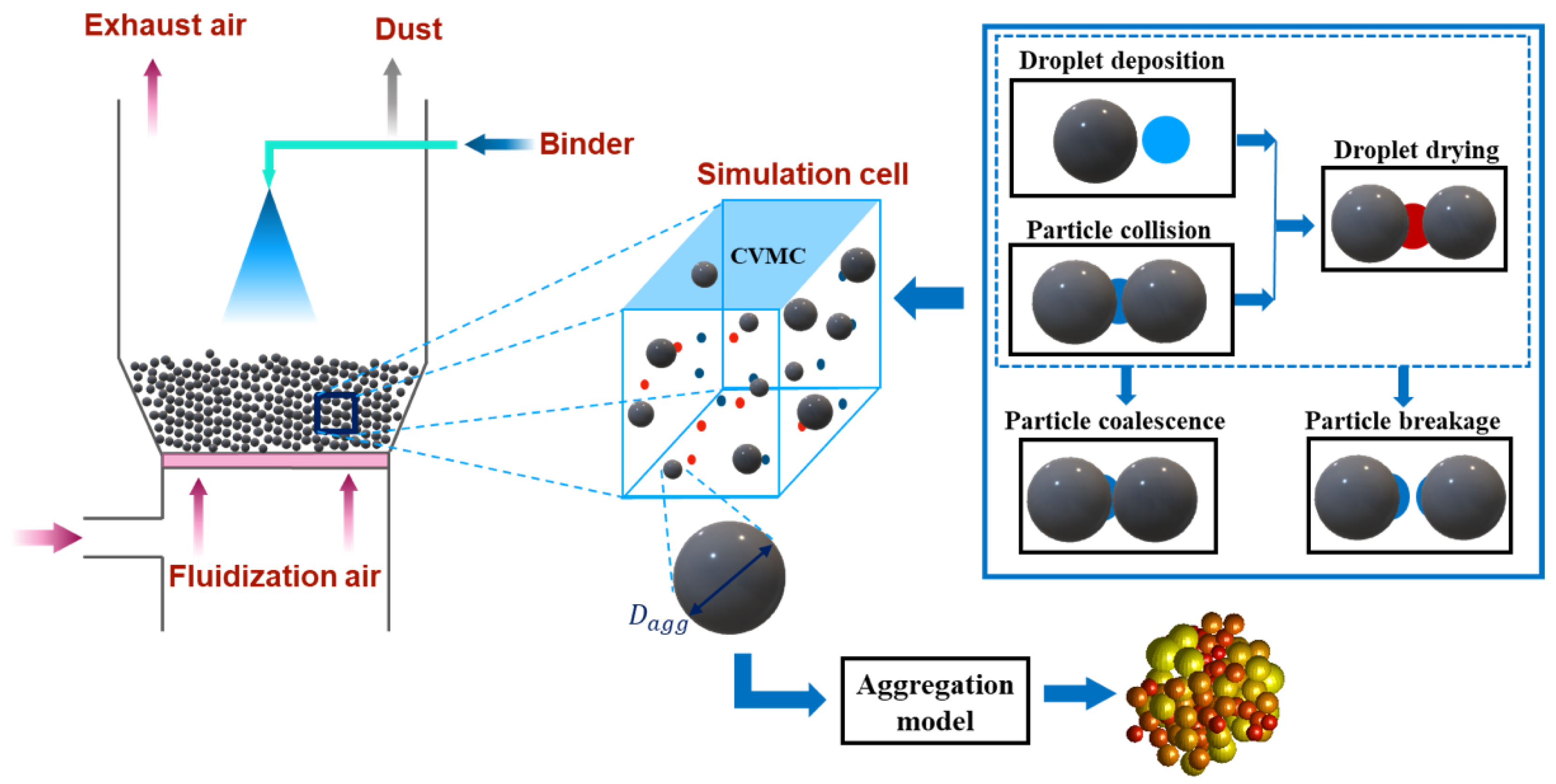
The simulation framework of CVMC, integrated with several micro-scale mechanisms, is given in Figure 1. The simulation cell, initially consisted of 1000 primary particles, was treated as a scaled-down virtual SFB agglomerator. The number of particles in the simulation cell varied according to the process, such as breakage or agglomeration, whichever prevailed during the simulation. In the case of agglomeration, when the particle number in the simulation cell becomes half, the periodic regulation of the particles is made by doubling the particle population.
At the start of the simulation, droplet deposition and particle collisions were set on instantaneously. The deposition of binder droplets takes place randomly on the particles (initially primary particles and later on agglomerates). Droplet drying occurs instantly after droplet deposition in SFB agglomeration. The reduction of the deposited liquid layer and, finally, the droplet loss is entirely because of the drying of the liquid binder droplet. Due to the droplet loss, the agglomeration rate is decreased. An agglomerate is formed when a successful collision occurs on the wet surfaces of primary particles. In order to capture the morphology of the agglomerate formed, each agglomerate is generated five times with the help of the aggregation model. The morphological properties of the agglomerates were then calculated and averaged over those five realizations. The CVMC simulation framework is briefly described in Appendix A. Further elaboration and validation of sub-models in the context of the CVMC simulation can be found in [30]. The aggregation model is presented in detail in the following section. The breakage model was taken from [27].
2.1. Aggregation Model
Basically, different kinds of aggregation models can be achieved by varying certain algorithm aspects. These can be classified into four categories: particle trajectories, aggregate formation, simulation lattice, and algorithm tuning [10,20].
Sticking probability and fractal properties are the two significant tuning parameters affecting the algorithm of particle aggregation. Sticking probability is the probability with which entities adhere to the main cluster [10,31]. The sticking probability is classed as one when the sticking of an entity takes place after every single collision with the main cluster. The resulting aggregates have a fractal structure and are tenuous with high porosity. The evaluated fractal dimension is close to 2.2, leading to the diffusion-limited aggregation model [32]. Sticking probability decreases as the number of collisions required to successfully aggregate the entities into the main cluster increases. The value of sticking probability can decrease to almost zero. The generated aggregates are then densely packed like a cube (on-lattice) or sphere (off-lattice). The evaluated fractal dimension is close to 3.0. This formation technique is called reaction-limited aggregation model [33].
Another tuning parameter is fractal properties, fractal dimension () and prefactor (k), of an aggregate. These are extracted using the scaling power law that provides the relationship between the number of primary particles of the agglomerates,, to their radii of gyration, ,
Here, is the mean radius of primary particles in an agglomerate. Assuming that the power law according to Equation (1) holds, primary particles are added to a cluster with a goal to achieve exact fractal properties. This aggregation process is named as the fractal tunable aggregation model.
2.1.1. Sticking Probability Model
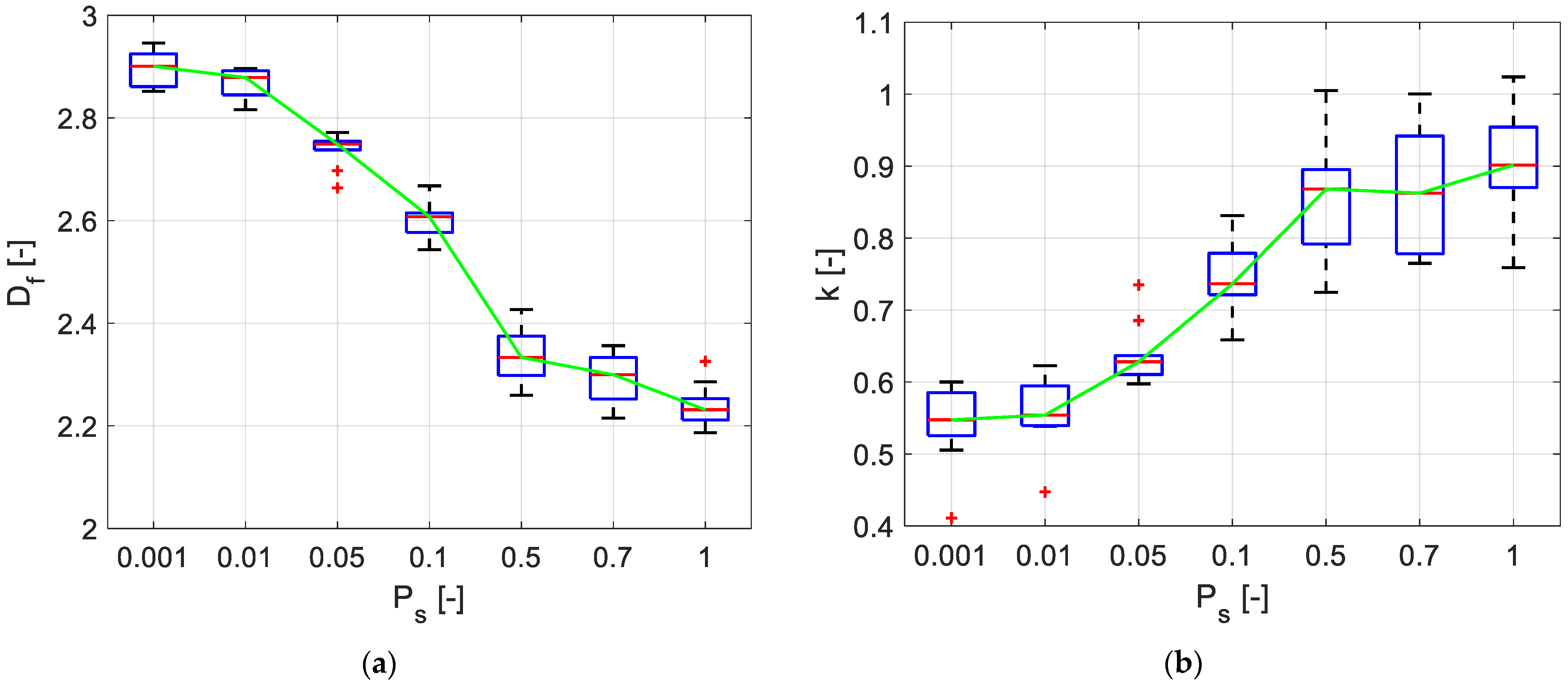
The sticking probability model is an on-lattice particle–cluster monodisperse aggregation model. A detailed algorithm of this model is given in [10,28]. A series of agglomerates consisting of spherical primary particles ranging from 5 to 100 in a step of 5 were generated by means of this model with a sticking probability of one. Then, the same series of agglomerates were developed at different values of the sticking probability (). Morphological descriptors, like fractal properties (fractal dimension and prefactor) and porosity (arithmetic mean over the series) of each series were evaluated. Each series of agglomerates was generated 10 times, and evaluated morphological descriptors are plotted in Figure 2 and Figure 3. The interquartile range (difference between the 75th and 25th percentile) for each series is represented by a box in Figure 2 and Figure 3. The median is indicated by the horizontal bar (highlighted in red) inside the box. The largest and lowest data points are represented by the horizontal bars (highlighted in black) at the top and bottom of the box, respectively. The outliers are indicated by a red plus sign. Figure 2 shows that the fractal dimension increased and the prefactor decreased as the sticking probability decreased.
A similar procedure was used to evaluate the porosity, calculated by the radius of gyration method, at various sticking probabilities. Figure 3 shows that with decreasing sticking probability, porosity also decreased. The lowest porosity obtained with this model is equivalent to the highest porosities examined for the largest SFB agglomerates in [34]. However, this porosity was still higher than the average porosity (around 0.6) of real SFB agglomerates examined in [34]. Moreover, as expected, the computation time to generate an agglomerate at a lower sticking probability increased for only a marginal change in the morphology [10,28].
The sticking probability model, being an on-lattice model, meant the generated agglomerates were more efficient. However, more realistic agglomerates can be generated by an off-lattice model (on a short scale) [5].
2.1.2. Fractal Tunable Aggregation Model
The basic framework of the tunable aggregation model is taken from the Huygens–Steiner theorem, which is used to calculate the moment of inertia of complex bodies. It states that any two parts of an arbitrary system (with total mass, and radius of gyration, ) satisfy the equation
where and are the masses of the two parts, is the distance between their centers of mass and and are the radii of gyration calculated by means of the scaling power law (given in Equation (1)).
Thus, by preserving both and , Equation (2) can be used to aggregate two clusters (or primary particle and aggregate) with at least one contact point and no overlapping between primary particles from the two adjoining clusters. For the new aggregate, is determined by substituting the value of from Equation (1) into Equation (2) and upon rearranging, it becomes
such that, and .
Equation (3) is the generalized equation for polydisperse cluster–cluster aggregation and is the same as given in [25]. Considering particle–cluster monodisperse aggregation, Equation (3) is simplified as
The radius of gyration of a solid sphere (considered in the middle term of right-hand side of Equation (4)) is not equivalent to its physical radius as used in [10,23,24,27]. Equation (4) is the corrected correlation for generating any particle–cluster monodisperse aggregate.
In the present work, a particle–cluster off-lattice modified polydisperse tunable sequential aggregation (MPTSA) algorithm is used. Polydisperse primary particles normally distributed with a given mean radius () and standard deviation are sequentially added for given fractal properties ( and ) as following:
- The radii of primary particles are normally distributed for a given number of primary particles ().
- The center of a 3D simulation space is allotted to the first primary particle from the distribution.
- Randomly, a point on the spherical surface of the first particle is selected and the second primary particle is brought into contact with it.
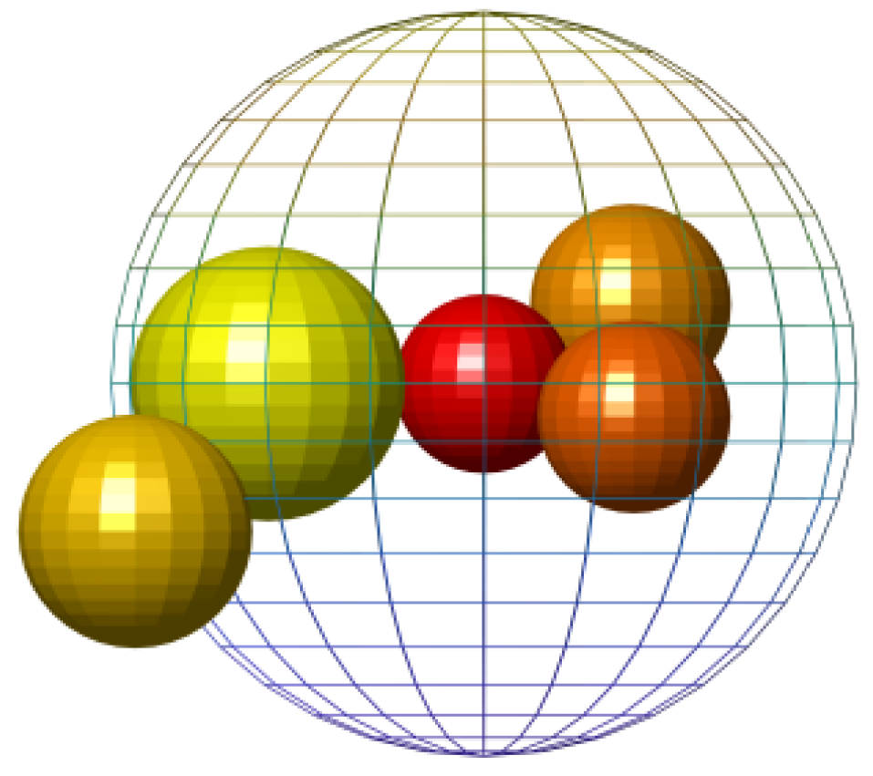
- The center of the third and subsequent particles is on a sphere of radius , which is obtained by modifying Equation (3) as,Here, N is from 3 to , is the radius of primary particle selected sequentially from the radius distribution and is the mass of the primary particle calculated from the corresponding radius. A schematic representation of the algorithm can be seen in Figure 4.
- A point is randomly selected on the surface of the sphere (of radius ), and the conditions for contact and overlap are checked.
- The new particle is attached to the growing cluster (initially with two particles), if there is contact without overlapping.
- Steps 5–7 are repeated until the condition is satisfied.
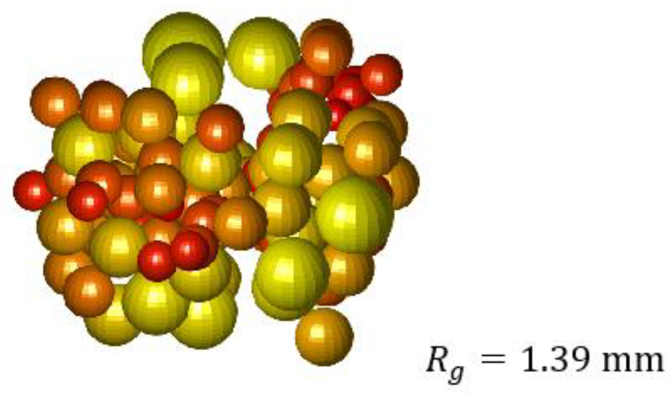
An illustration of this algorithm is shown in Figure 5 by generating an agglomerate (with ). The input fractal parameters are and , and radius of primary particles normally distributed (with μm and μm). The radius of gyration of the agglomerate is determined from the formulation given by [35],
Previous particle–cluster tunable aggregation models [10,23,24,27] assumed the radius of the primary particle as its radius of gyration in Equation (3), which has been correctly used in the present work (Equation (4)). In our previous work [24,27], an assumption was made in the algorithm (, (Equation (4)) regarding the mass of the individual polydisperse primary particles. The masses of polydisperse primary particles were assumed the same. This assumption is replaced in the present work by introducing the masses of individual primary particles (, (Equation (6)), similar to the algorithm proposed in [25]. However, the algorithm from [25] was not able to generate agglomerates resembling real SFB agglomerates, like those from [29]. The reason could be combinations of large with small k (prefactor limitation) in [25].
The limitation of prefactor is also resolved in the MPTSA model by tuning the fractal dimension at a fixed prefactor using the correlation derived by Singh and Tsotsas [10]. This correlation was based not only on the porosity correlation of agglomerates with monodisperse primary particles, but also on the power law; we know that the power law depends on the mean radius of the primary particle in an aggregate and not on the individual radius. Thus, the tuning fractal dimension correlation (Equation (5)) can be extended to aggregates with polydisperse primary particles.
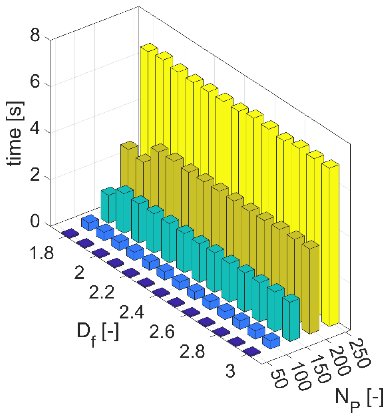
Figure 6 shows the simulation time required to generate agglomerates with monodisperse primary particles in increments of 50 from 50 to 250 using the MPTSA model. is taken from 1.8 to 3 in steps of 0.1 and k is fixed at 1. An agglomerate with 100 polydisperse spherical primary particles takes less than 1 s to generate on a typical personal computer (with 4 cores, 4 GB RAM, and 3.4 GHz processor). The modified polydisperse tunable sequential aggregation (MPTSA) model is computationally faster than previous models [10,27].
3. Results and Discussion
3.1. Validation of MPTSA Model
The experimental SFB agglomerates examined by Dadkhah [29] were used to validate the MPTSA model. The primary particles used in her experiments were glass beads, with hydroxypropylmethylcellulose (HPMC) in an aqueous solution as the binder. All her experiments with various morphological descriptors obtained are briefly presented in Appendix B.
The radii of the glass beads were measured with Camsizer and showed a Gaussian distribution with a standard deviation of about 10% of the mean particle radius. The findings of Dadkhah’s experiments tabulated in Table A1 and measured by X-ray tomography indicate that the primary particles evaluated for individual agglomerates were normally (Gaussian) distributed with a standard deviation of 30 μm and 3 μm (i.e., 10% and 1% of mean radius of the primary particle) for experiments A and B, respectively.
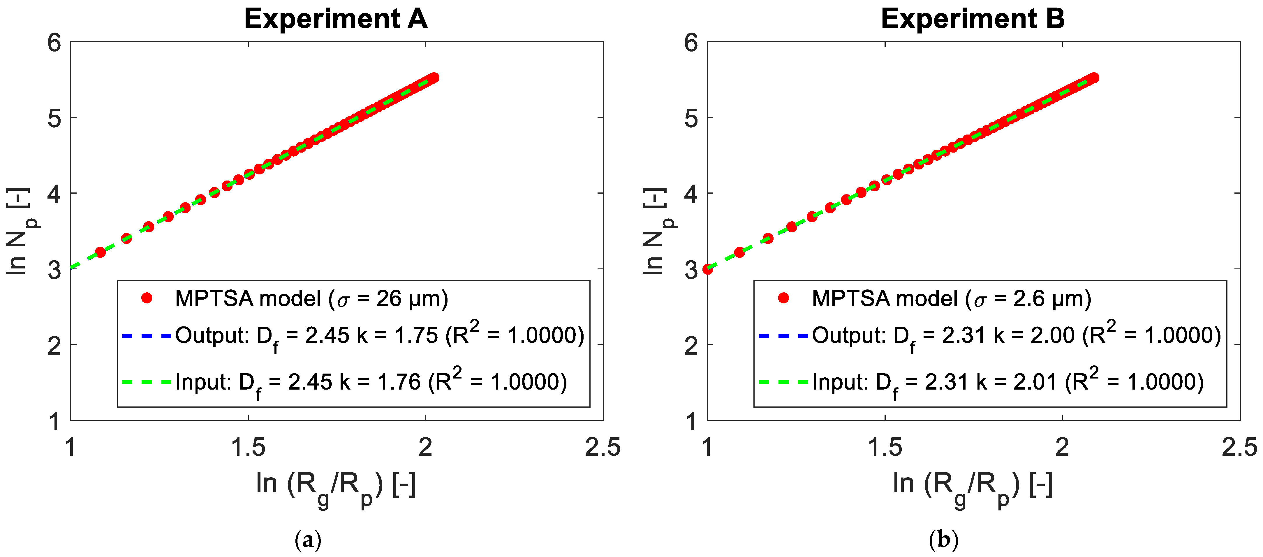
Accordingly, for experiments A and B, a standard deviation of 26 μm and 2.6 μm, respectively, has been used in combination with a mean radius of 260 μm to generate the Gaussian distribution of the primary particles in the MPTSA model. Based on this distribution, a series of agglomerates with the number of primary particles ranging from 20 to 250 at a regular increment of 5 have been constructed by employing the MPTSA model. The input values of fractal dimension and prefactor are taken from Table A1 for respective experiments. The radius of gyration for each agglomerate generated with the MPTSA model has been calculated using Equation (7). Then, it is averaged over five realizations and plotted on a double logarithmic scale, given in Figure 7, against the number of primary particles for each experiment. and of the series of agglomerates (constructed by means of the MPTSA model) are calculated from the power law relationship on a double logarithmic scale for the entire sample. This evaluation method is consistent with the evaluation method of Dadkhah et al. [36].
Figure 7 shows the fractal properties obtained using the power law for agglomerates generated by employing the MPTSA model, denoted as output, are preserved accurately compared to the corresponding input fractal properties for Exp. A and Exp. B, respectively. The power law is perfectly satisfied in both cases, with for the output (generated using the MPTSA model) and for the respective input fractal properties. Moreover, the extracted fractal properties (output) are almost identical for experiment B with a standard deviation of 1% of mean radius () and also for Exp. A with . The retention of the fractal properties and resemblance with the power law is excellent, validating the model. Furthermore, the extracted fractal properties ( and for Exp. A from the MPTSA model are more accurate than the extracted fractal properties ( and from Singh and Tsotsas [27] with the corresponding, same input fractal properties ( and .
3.2. MPTSA Model
Several agglomerates were constructed by means of the MPTSA model by varying the number of primary particles in a range from 20 to 250 with a step size of 5. The input fractal properties ( and ) required by the MPTSA model for each trial were taken from the respective experiment according to Table 1. It can be seen from Table A1, as well as Figure A1, that the radii of the primary particles determined by Dadkhah were actually normally distributed with a standard deviation of around 10% of the mean radius. Correspondingly, the radii of primary particles were normally distributed with μm and μm (10% of the mean radius) and were used in the MPTSA model.
The morphological descriptors were determined and averaged over five realizations for agglomerates generated from the MPTSA model. Fractal properties ( and ) of the agglomerates were obtained by means of the power law relationship (Equation (1)) on a double logarithmic scale for the entire sample. This evaluation technique is consistent with the method used in [10,34]. The porosity of the agglomerate () was calculated from the radius of gyration method. For each agglomerate in a series, values of porosity and mean coordination number (MCN) were calculated, then arithmetically averaged for the series, then averaged over five realizations, and finally, listed in Table 1. This procedure is also consistent with the technique used in evaluating the tomography data by Dadkhah [29].
Morphological descriptors obtained with the MPTSA model are better than those obtained by Singh and Tsotsas [10] and are in close affinity with the experimental values [34]. The fractal properties were preserved accurately. A slight deviation in the average porosity and MCN results from the MPTSA model was due to the sample of agglomerates used in the experiments [29] (i.e., about 25 agglomerates selected randomly), while in simulations, the primary particles ranged from 20 to 250 with a regular increment of 5 (i.e., 47 agglomerates in equal intervals). However, morphological changes in the agglomerates generated by the MPTSA model at different operating parameters were in great accordance with the real agglomerates from [34].
3.3. CVMC Model
Experiments from Table A1 have been simulated for 10 min by means of the CVMC model. Corresponding experimental parameters and simulation parameters are the same as in [9,10,27] and are summarized in Table 2. Agglomerates were generated using the MPTSA model. Primary particles were distributed normally with a mean radius of primary particles, μm, and μm. Input fractal properties ( and ) for the MPTSA model were calculated using the empirical correlations developed in [9,10] by inserting binder concentration and inlet temperature of fluidized gas for respective trials from Table A1.
3.3.1. Agglomerate Kinetics
Time is an important factor and is shown in Table 3 and in Figure 8. In Table 3, the growth rate is evaluated using the present CVMC simulation with the MPTSA model and compared with experiments [29] and previous CVMC simulation with the polydisperse TSA model [27]. With the help of the overall growth rate, kinetics of the process at different binder concentrations, and inlet temperatures is expressed.
The overall growth rate in Table 3 is calculated using:
Here, is Sauter mean radius of the particle population in the simulation cell at the end of the process (i.e., 10 min), is the mean radius of primary particles, and is the duration of the trial. The radius of the formed agglomerates is calculated using surface area equivalent sphere,
where is the surface area calculated with the convex hull method, by generating the agglomerates from the MPTSA model.
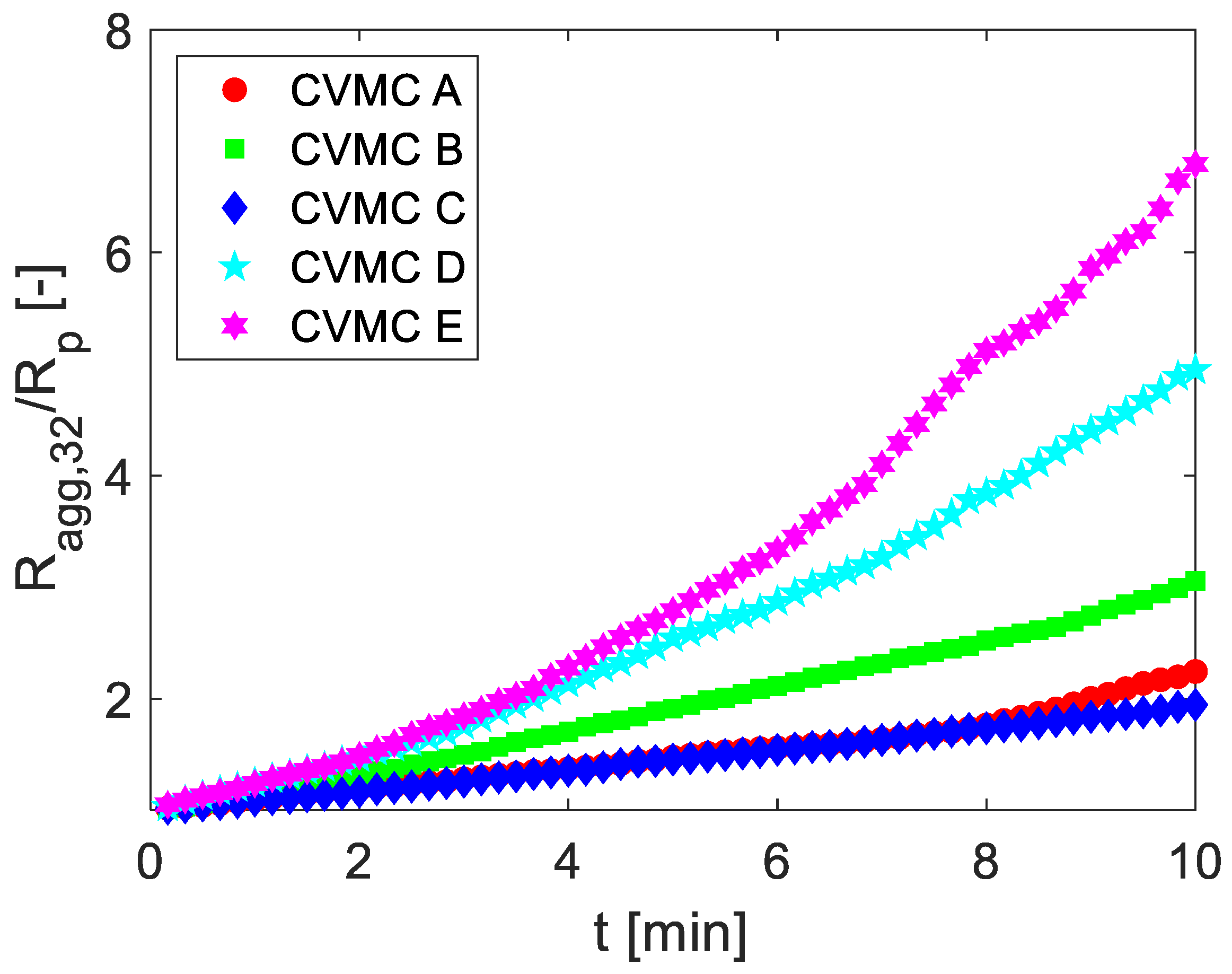
Figure 8 shows the temporal growth, expressed in terms of the relative agglomerate radius (ratio of Sauter mean radius of the particle population and the initial radius) over time, for different experiments by means of the CVMC model. It can be assessed from Figure 8 (and also from Table 3) that; the growth rate decreased as the temperature of the inlet fluidized gas increased (Exp. B, A, and C with increasing temperature). The reason behind this is that at a higher temperature of the fluidizing gas, the drying of the binder droplets is faster. The droplet size decreases as the temperature increases and the probability of particles colliding at wet areas decreases. As a result, the agglomeration rate decreased. Additionally, droplet loss was also very pronounced at high temperatures. This also leads to a reduction in the agglomeration rate.
With increasing binder concentration (from Exp. A, to Exp. D, and finally to Exp. E), the viscosity of the binder droplet increases and it becomes easier to fulfill the Stokes criterion during impact on wet surfaces. A higher proportion of the collision energy is dissipated by a more viscous liquid. Consequently, the agglomeration growth rate increases, as depicted in Figure 8. The overall kinetics under different operating conditions is decreased slightly by implementing the improved aggregation model (MPTSA) compared to our previous work [24,27].
3.3.2. Agglomerate Morphology
The morphology of the agglomerates is also influenced by changing the process parameters. Figure 9 shows the largest agglomerates formed in different experiments at the end of the simulation (i.e., after 10 min). As concluded in Section 3.3.1, the agglomeration rate is highest for Exp. E and lowest for Exp. C. This can also be seen in Figure 9 with respect to the number of primary particles in respective agglomerates.
With increasing temperature (from Exps. B to A and, finally, to C), the binder droplets become smaller due to faster drying. The liquid bridges formed after successful particle collisions by smaller droplets are also smaller and easier to break. In order to stabilize the formed agglomerates, more bridges are necessary, resulting in more compact structures. Therefore, at high temperatures, the fractal dimension is higher and the agglomerate porosity is lower, which in turn reduces the radius of the final formed agglomerates, making them more compact.
The influence of increasing the binder concentration (from Exps. A to D and, finally, to E) on the morphology can also be explained. Binder with a high concentration is more viscous and the bridges formed are stronger than those with a low concentration. At high binder concentration, the agglomerates formed have a high probability of surviving in the SFB as they are loosely arranged in space. Due to the loose arrangement of primary particles, the agglomerates are large, porous, and tenuous. Therefore, at high binder concentration, the fractal dimension is smaller and the agglomerate porosity is higher.
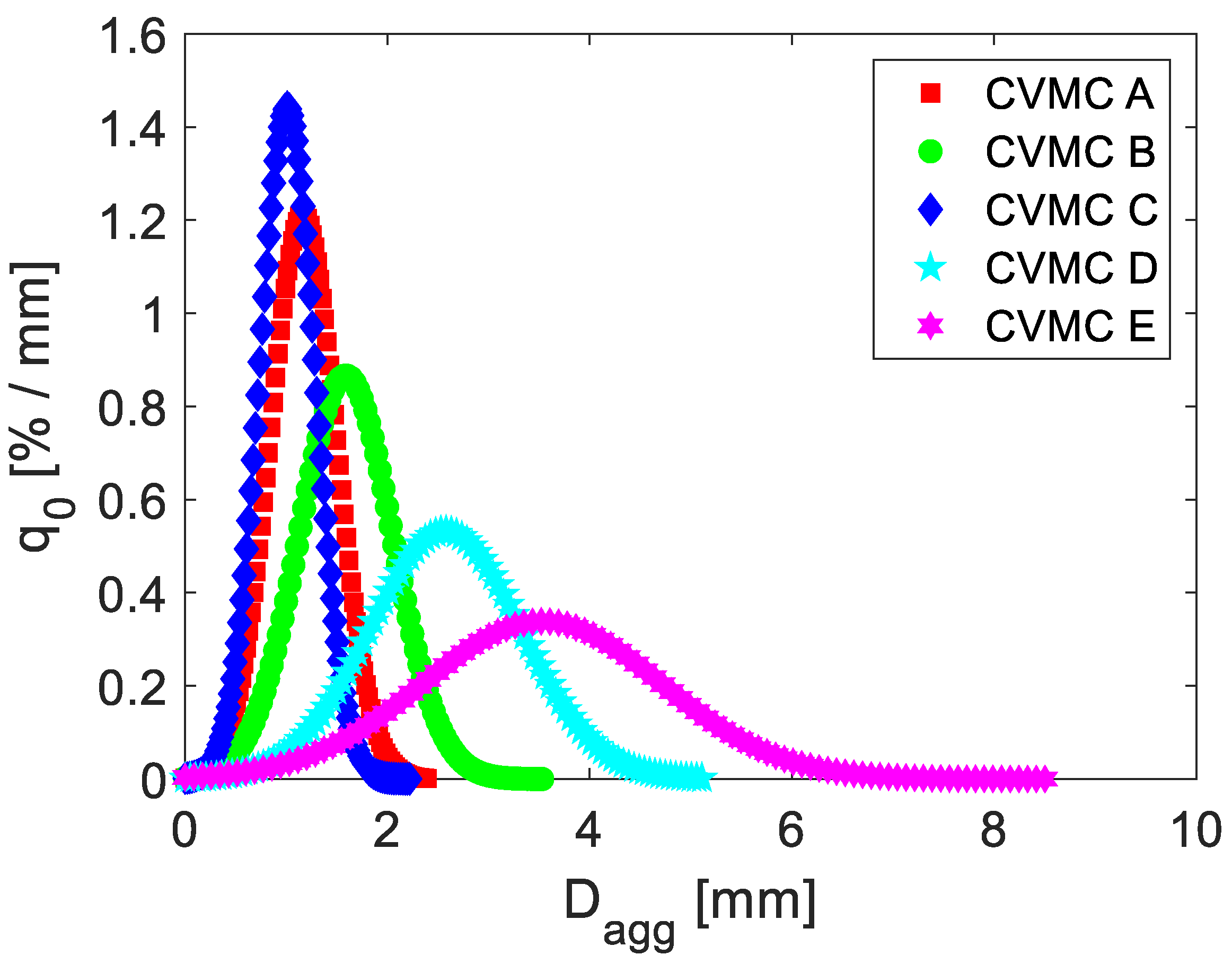
The particle size distributions for different experiments after 10 min of CVMC simulations are shown in Figure 10. At high temperature, the agglomerates formed are small, so PSD is narrower and is shifted to the left with increasing temperature from experiments B to A and, finally, to C. On the contrary, PSD is always broader at low fractal dimensions. The reason behind this is the formation of large and porous agglomerates with high porosity. Therefore, PSD is shifted to the right with increasing binder mass fraction from experiments A to D and, finally, to E. These distributions are consistent with the experimental results of Dadkhah [29].
4. Conclusions
The tendency of the sticking probability model to generate agglomerates with excessively high porosities motivated us to develop a model that could better tune morphological descriptors. Therefore, a modified polydisperse tunable aggregation model has been developed using the correct expression to calculate the distance of the new approaching particle. The numerical algorithm of the MPTSA model to reconstruct the SFB agglomerates with polydisperse primary particles is based on power law and radius of gyration. The influence of polydispersity cannot be depicted entirely using the power law, since it is based on the mean radius of the primary particles in an agglomerate.
Fractal properties ( and ) were accurately preserved for agglomerates with a standard deviation of 10% from the mean primary particle size, which roughly corresponds to the available experimental results. The morphological properties of agglomerates examined by Dadkhah have been investigated in detail by means of the MPTSA model. Irrespective of each agglomerate having tuned fractal dimension in the MPTSA model, fractal properties extracted for reconstructed agglomerates were better than those provided by previous aggregation models [10,27] and agreed exactly with the fractal properties of experimental agglomerates [29]. Other morphological parameters, like mean coordination number and porosity obtained from the MPTSA model, were also better as compared to those provided by previous aggregation models [10,27] and strongly agreed with the experiments. The MPTSA model is not based on any forces and, therefore, can be easily used to mimic the morphology of aggregates ranging from nanoscale to macro-scale.
In order to investigate the growth kinetics of the process, this structure formation algorithm has been integrated with the comprehensive stochastic simulation framework (CVMC). The present CVMC simulation, with the improved polydisperse tunable sequential aggregation model, satisfactorily predicts the morphological descriptors of SFB agglomerates as well as the overall growth kinetics of SFB agglomeration under various operating parameters. The overall kinetics does not differ significantly after the implementation of the improved aggregation model, but the morphology is mimicked better as compared to previous models [10,27].
Present work could serve as a foundation to further investigate the growth kinetics and morphology of soft and/or porous agglomerates. This study might also be extended to examine the morphological properties of heteroagglomerates that consist of more than one type of primary particle.
Author Contributions
Conceptualization, A.K.S. and E.T.; methodology, A.K.S.; software, A.K.S.; validation, A.K.S.; formal analysis, A.K.S.; investigation, A.K.S.; resources, A.K.S.; data curation, A.K.S.; writing—original draft preparation, A.K.S.; writing—review and editing, E.T.; visualization, A.K.S.; supervision, E.T.; project administration, E.T.; funding acquisition, E.T. All authors have read and agreed to the published version of the manuscript.
Funding
This research was funded by the Bundesministerium für Bildung und Forschung (BMBF), as a part of the combined agglomeration technology for food (COAGG) project (03INT609AA) in the frame of the excellence cluster “Wirbelschicht- und Granuliertechnik” (WIGRATEC).
Conflicts of Interest
The authors declare no conflict of interest.
Appendix A. CVMC Model after Singh, A.K. and Tsotsas, E., 2022
After every collision event, the time step is computed using
with the collision frequency [30]
where is the collision frequency prefactor, and are the solid volume fractions of the fixed bed and the expanded bed, respectively, is the fluidization velocity. is assumed to be 0.61. is calculated using [2],
Here, is Reynolds number and is Archimedes number. These are particle dimensionless numbers adopted from [2,16].
Binder droplets (with HPMC binder in aqueous solution) are continuously deposited on the fluidized particles. The CVMC model is related to the real process by the concentration of droplets per unit time and primary particle () inside the simulation box and the actual process. in the real process is
where is spray mass flow rate, is bed mass, and are densities of primary particle density and liquid, respectively, and are diameter (twice the mean radius, ) of primary particle and droplet, respectively. Deposition of a liquid droplet on a particle depends on its surface energy and contact angle. At a contact angle θ = 0°, the deposited droplet spreads out entirely and forms a film layer. For θ > 0°, it partially wets the surface of the particle and takes the form of a spherical cap with a base radius
and initial height
A contact angle made by the binder droplet deposited on the non-porous glass beads used as primary particles is taken as . Deposited droplet on the particle (initially primary particle and later agglomerate) evaporates immediately and eventually solidifies. Drying of deposited droplets is modeled using temporal reduction of droplet height as
where and , and and , are the molar masses and mass densities of gas (air) and water, respectively, is the mass transfer coefficient; and are the system pressure and the saturation vapor pressure, respectively. , is the molar fraction of water in the gas phase and is calculated from gas moisture content ,
In order to obtain , it is assumed that the SFB is perfectly mixed and that the amount of water evaporated from the binder droplets at any time is always equal to the amount of water sprayed through the nozzle.
Coalescence between agglomerates or primary particles occurs when their initial kinetic energy is less than the energy due to the viscosity of the liquid binder layer of the droplet. The critical conditions to dissipate the kinetic energy through a viscous layer were first derived in [37] in terms of Stokes number
Here is particle collision velocity, is the binder viscosity as a function of binder concentration [27], and are combined mass and diameter of colliding particles of unequal size, respectively, and calculated using:
Two colliding particles will coalesce if the actual Stokes number is smaller than the critical Stokes number [38]
Particle collisions within the fluidized bed promote not only coalesce, but also breakage of already formed agglomerates is seen. Breakage of an agglomerate happens when the Stokes deformation number
is greater than the critical Stokes deformation number
Here is calculated from Singh and Tsotsas [27]
where, and are mean coordination number and porosity of the agglomerate, respectively. These quantities are obtained by generating the agglomerate using the MPTSA model.
Particle collision velocity () is a significant parameter in determining the Stokes numbers. In this present work, is chosen randomly by assuming a normal distribution of particle velocity with a standard deviation of 0.1 m/s and a mean value of . This coarse assumption of particle collision velocity was taken from the previous work [30], where it described the experimental results quite successfully. Further optimization is possible, but beyond the scope of this study.
Appendix B. Experiments of Dadkhah, M., 2014
A laboratory-scale fluidized bed agglomerator was used in the experiments of Dadkhah [29]. The height and the inner diameter of the agglomerator were 450 mm and 152 mm, respectively. A two-fluid nozzle in top spray configuration was used and was located 150 mm above the air distributor plate. Droplets consisted of Hydroxypropylmethylcellulose (HPMC) binder dissolved in water, injected through the nozzle.

Table A1.
Experimental findings for each trial.
| A | B | C | D | E | |
|---|---|---|---|---|---|
| Temperature [℃] | 60 | 30 | 90 | 60 | 60 |
| Binder [wt.%] | 2 | 2 | 2 | 6 | 10 |
| [-] | 2.45 | 2.31 | 2.94 | 2.24 | 2.09 |
| k [-] | 1.76 | 2.01 | 0.98 | 1.96 | 2.24 |
| [-] | 0.57 | 0.62 | 0.53 | 0.58 | 0.63 |
| [-] | 3.32 | 3.10 | 4.02 | 2.92 | 2.87 |
| Evaluated agglomerates | 25 | 28 | 22 | 24 | 24 |
| [μm] | (321.2 236.8) | (317.3 303.3) | (298.6 210.4) | (342.9 229.5) | (332.0 300.3) |
| [μm] | 288.2 | 309.3 | 257.3 | 285.3 | 312.4 |
| [μm] | 30 | 3 | 33 | 32 | 9 |
Five experiments with glass beads as primary particles were carried out to investigate the influence of process parameters (initial binder concentration and inlet fluidized gas temperature). The experiments are listed in Table A1, where Exp. A is the reference experiment with a binder concentration of 2% and inlet fluidized gas temperature of 60 °C. Binder concentration is increased from 2% in Experiment A to 6% in Experiment D and finally to 10% corresponding to Experiment E. Inlet temperature of the fluidized gas is varied from 30 °C to 60 ℃ and finally to 90 °C that corresponds to experiments B, A and C, respectively.
The morphological descriptors (, k, average , average MCN) determined for different experiments are also listed in Table A1. For each experiment, these descriptors were derived by examining about 24 agglomerates (the exact number of agglomerates examined for each experiment is given in Table A1).
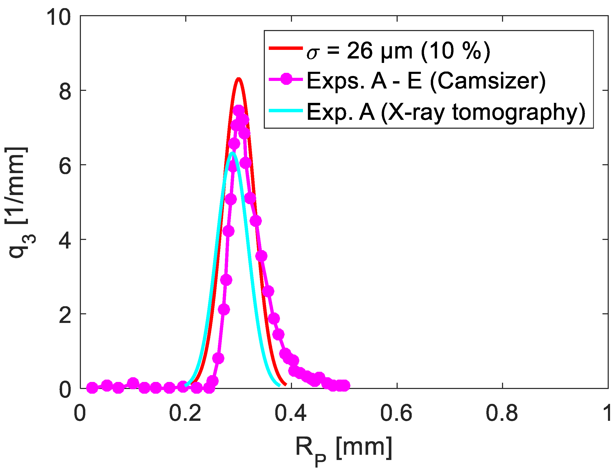
The sphericity of the non-porous glass beads was very high (0.98). Size distributions of glass beads were measured with Camsizer and are shown in Figure A1. The radii of glass beads have a normal distribution with a standard deviation of around 10% from the mean radius of 260 μm. Radii of glass beads were also determined from X-ray tomography data of individual agglomerates from different experiments and are listed in Table A1 (and in Figure A1; for experiment A). The standard deviation of the primary particle radius from X-ray tomography data agrees with the Camsizer data, i.e., it is around 10% of the arithmetic mean radius for all the experiments except Exps. B and E with 1% and 3%, respectively.
Figure A1.
PSD of glass beads measured by Camsizer and primary particles determined from X-ray tomography data of individual agglomerates of Exp. A.
Figure A1.
PSD of glass beads measured by Camsizer and primary particles determined from X-ray tomography data of individual agglomerates of Exp. A.

References
- Peglow, M.; Antonyuk, S.; Jacob, M.; Palzer, S.; Heinrich, S.; Tsotsas, E. Particle formulation in spray fluidized beds. In Modern Drying Technology; Wiley-VCH Verlag GmbH & Co. KGaA: Weinheim, Germany, 2014; pp. 295–378. [Google Scholar]
- Mörl, L.; Heinrich, S.; Peglow, M. Fluidized bed spray granulation. In Handbook of Powder Technology; Elsevier: Amsterdam, The Netherlands, 2007; Volume 36, pp. 21–188. [Google Scholar]
- Dernedde, M.; Peglow, M.; Tsotsas, E. Stochastic modeling of fluidized bed agglomeration: Determination of particle moisture content. Dry. Technol. 2013, 31, 1764–1771. [Google Scholar] [CrossRef]
- Kumar, J. Numerical Approximations of Population Balance Equations in Particulate Systems. Ph.D. Thesis, Otto von Guericke University, Magdeburg, Germany, 2006. [Google Scholar]
- Peglow, M.; Kumar, J.; Hampel, R.; Tsotsas, E.; Heinrich, S. Towards a complete population balance model for fluidized bed spray agglomeration. Dry. Technol. 2007, 25, 1321–1329. [Google Scholar] [CrossRef]
- Terrazas-Velarde, K.; Peglow, M.; Tsotsas, E. Kinetics of fluidized bed spray agglomeration for compact and porous particles. Chem. Eng. Sci. 2011, 66, 1866–1878. [Google Scholar] [CrossRef]
- Dernedde, M.; Peglow, M.; Tsotsas, E. A novel, structure-tracking Monte Carlo algorithm for spray fluidized bed agglomeration. AIChE J. 2012, 58, 3016–3029. [Google Scholar] [CrossRef]
- Rieck, C.; Schmidt, M.; Bück, A.; Tsotsas, E. Monte Carlo modeling of binder-Less spray agglomeration in fluidized beds. AIChE J. 2018, 64, 3582–3594. [Google Scholar] [CrossRef]
- Singh, A.K.; Tsotsas, E. Stochastic model to simulate spray fluidized bed agglomeration: A morphological approach. Powder Technol. 2019, 355, 449–460. [Google Scholar] [CrossRef]
- Singh, A.K.; Tsotsas, E. A tunable aggregation model incorporated in Monte Carlo simulations of spray fluidized bed agglomeration. Powder Technol. 2020, 364, 417–428. [Google Scholar] [CrossRef]
- Dosta, M.; Antonyuk, S.; Heinrich, S. Multiscale simulation of agglomerate breakage in fluidized beds. Ind. Eng. Chem. Res. 2013, 52, 11275–11281. [Google Scholar] [CrossRef]
- Jiang, Z.; Bück, A.; Tsotsas, E. CFD–DEM study of residence time, droplet deposition, and collision velocity for a binary particle mixture in a Wurster fluidized bed coater. Dry. Technol. 2018, 36, 638–650. [Google Scholar] [CrossRef]
- Sommerfeld, M.; Stübing, S. A novel Lagrangian agglomerate structure model. Powder Technol. 2017, 319, 34–52. [Google Scholar] [CrossRef]
- Köylu, Ü.; Xing, Y.; Rosner, D.E. Fractal Morphology Analysis of Combustion-Generated Aggregates Using Angular Light Scattering and Electron Microscope Images. Langmuir 1995, 11, 4848–4854. [Google Scholar] [CrossRef]
- Breuer, M.; Almohammed, N. Modeling and simulation of particle agglomeration in turbulent flows using a hard-sphere model with deterministic collision detection and enhanced structure models. Int. J. Multiph. Flow 2015, 73, 171–206. [Google Scholar] [CrossRef]
- Terrazas-Velarde, K.; Peglow, M.; Tsotsas, E. Investigation of the kinetics of fluidized bed spray agglomeration based on stochastic methods. AIChE J. 2011, 57, 3012–3026. [Google Scholar] [CrossRef]
- Thouy, R.; Jullien, R. A cluster-cluster aggregation model with tunable fractal dimension. J. Phys. A. Math. Gen. 1994, 27, 2953–2963. [Google Scholar] [CrossRef]
- Mackowski, D.W. Electrostatics analysis of radiative absorption by sphere clusters in the Rayleigh limit: Application to soot particles. Appl. Opt. 1995, 34, 3535. [Google Scholar] [CrossRef]
- Chakrabarty, R.K.; Garro, M.A.; Chancellor, S.; Herald, C.; Moosmüller, H. FracMAP: A user-interactive package for performing simulation and orientation-specific morphology analysis of fractal-like solid nano-agglomerates. Comput. Phys. Commun. 2009, 180, 1376–1381. [Google Scholar] [CrossRef]
- Kätzel, U.; Bedrich, R.; Stintz, M.; Ketzmerick, R.; Gottschalk-Gaudig, T.; Barthel, H. Dynamic light scattering for the characterization of polydisperse fractal systems, Part 1: Simulation of the diffusional behavior. Part. Part. Syst. Charact. 2008, 25, 9–18. [Google Scholar] [CrossRef]
- Brasil, A.M.; Farias, T.L.; Carvalho, M.G.; Koylu, U.O. Numerical characterization of the morphology of aggregated particles. J. Aerosol Sci. 2001, 32, 489–508. [Google Scholar] [CrossRef]
- Sorensen, C.M.; Roberts, G.C. The prefactor of fractal aggregates. J. Colloid Interface Sci. 1997, 186, 447–452. [Google Scholar] [CrossRef]
- Filippov, A.V.; Zurita, M.; Rosner, D.E. Fractal-like aggregates: Relation between morphology and physical properties. J. Colloid Interface Sci. 2000, 229, 261–273. [Google Scholar] [CrossRef] [PubMed]
- Skorupski, K.; Mroczka, J.; Wriedt, T.; Riefler, N. A fast and accurate implementation of tunable algorithms used for generation of fractal-like aggregate models. Phys. A Stat. Mech. Its Appl. 2014, 404, 106–117. [Google Scholar] [CrossRef]
- Morán, J.; Fuentes, A.; Liu, F.; Yon, J. FracVAL: An improved tunable algorithm of cluster–cluster aggregation for generation of fractal structures formed by polydisperse primary particles. Comput. Phys. Commun. 2019, 239, 225–237. [Google Scholar] [CrossRef]
- Morán, J.; Yon, J.; Poux, A. Monte Carlo Aggregation Code (MCAC), Part 1: Fundamentals. J. Colloid Interface Sci. 2020, 569, 184–194. [Google Scholar] [CrossRef] [PubMed]
- Singh, A.K.; Tsotsas, E. Influence of polydispersity and breakage on stochastic simulations of spray fluidized bed agglomeration. Chem. Eng. Sci. 2022, 247, 117022. [Google Scholar] [CrossRef]
- Singh, A.K. Morphology Based Stochastic Simulation of Spray Fluidized Bed Agglomeration. Ph.D. Thesis, Otto-von-Guericke-Universität, Magdeburg, Germany, 2021. [Google Scholar]
- Dadkhah, M. Morphological Characterization of Agglomerates Produced in a Spray Fluidized Bed by X-Ray Tomography. Ph.D. Thesis, Otto von Guericke University, Magdeburg, Germany, 2014. [Google Scholar]
- Terrazas-Velarde, K.; Peglow, M.; Tsotsas, E. Stochastic simulation of agglomerate formation in fluidized bed spray drying: A micro-scale approach. Chem. Eng. Sci. 2009, 64, 2631–2643. [Google Scholar] [CrossRef]
- Turkevich, L.A.; Scher, H. Sticking probability scaling in diffusion-limited aggregation. In Fractals in Physics; Elsevier: Amsterdam, The Netherlands, 1986; pp. 223–229. ISBN 9781604138795. [Google Scholar]
- Meakin, P. Historical introduction to computer models for fractal aggregates. J. Sol-Gel Sci. Technol. 1999, 15, 97–117. [Google Scholar] [CrossRef]
- Eden, M. A two-dimensional growth process. In Proceedings of the 4th Berkeley Symposium on Mathematical Statistics and Probability, Berkeley, CA, USA, 20 June–30 July 1960; University of California Press: Berkeley, CA, USA, 1961; Volume 4, pp. 223–239. [Google Scholar]
- Dadkhah, M.; Tsotsas, E. Influence of process variables on internal particle structure in spray fluidized bed agglomeration. Powder Technol. 2014, 258, 165–173. [Google Scholar] [CrossRef]
- Dastanpour, R.; Rogak, S.N. The effect of primary particle polydispersity on the morphology and mobility diameter of the fractal agglomerates in different flow regimes. J. Aerosol Sci. 2016, 94, 22–32. [Google Scholar] [CrossRef] [Green Version]
- Dadkhah, M.; Peglow, M.; Tsotsas, E. Characterization of the internal morphology of agglomerates produced in a spray fluidized bed by X-ray tomography. Powder Technol. 2012, 228, 349–358. [Google Scholar] [CrossRef]
- Davis, R.H.; Serayssol, J.-M.; Hinch, E.J. The elastohydrodynamic collision of two spheres. J. Fluid Mech. 1986, 163, 479–497. [Google Scholar] [CrossRef] [Green Version]
- Barnocky, G.; Davis, R.H. Elastohydrodynamic collision and rebound of spheres: Experimental verification. Phys. Fluids 1988, 31, 1324–1329. [Google Scholar] [CrossRef]
Figure 1.
CVMC simulation framework for SFB agglomeration.

Figure 2.
The fractal dimension (a) and prefactor (b) of agglomerates constructed by employing the sticking probability model at different sticking probabilities ().
Figure 2.
The fractal dimension (a) and prefactor (b) of agglomerates constructed by employing the sticking probability model at different sticking probabilities ().

Figure 3.
Porosity obtained from the radius of gyration method for agglomerates generated by employing the sticking probability model at different sticking probabilities ().
Figure 3.
Porosity obtained from the radius of gyration method for agglomerates generated by employing the sticking probability model at different sticking probabilities ().

Figure 4.
An illustration of the MPTSA algorithm with solid spheres as polydisperse primary particles (; red for the smallest (197 μm) and yellow for the largest (340 μm) primary particle) and a hollow sphere of radius for the addition of a sixth primary particle.
Figure 4.
An illustration of the MPTSA algorithm with solid spheres as polydisperse primary particles (; red for the smallest (197 μm) and yellow for the largest (340 μm) primary particle) and a hollow sphere of radius for the addition of a sixth primary particle.

Figure 5.
An exemplary agglomerate (with ; red for the smallest (122 μm) and yellow for the largest (396 μm) primary particle) generated using the MPTSA model (with μm and μm).
Figure 5.
An exemplary agglomerate (with ; red for the smallest (122 μm) and yellow for the largest (396 μm) primary particle) generated using the MPTSA model (with μm and μm).

Figure 6.
Simulation time required to generate agglomerates (with ; ; ) by employing the MPTSA model (with μm and μm).
Figure 6.
Simulation time required to generate agglomerates (with ; ; ) by employing the MPTSA model (with μm and μm).

Figure 7.
Preservation of fractal properties of agglomerates constructed by means of the MPTSA model for Exp. A (a) and Exp. B (b).
Figure 7.
Preservation of fractal properties of agglomerates constructed by means of the MPTSA model for Exp. A (a) and Exp. B (b).

Figure 8.
Temporal growth of particles by employing the CVMC simulation for the different experiments.
Figure 8.
Temporal growth of particles by employing the CVMC simulation for the different experiments.

Figure 9.
Largest agglomerate (with the number of primary particles; red denoting the smallest, and yellow the largest primary particle, ) formed after 10 min of CVMC simulations for different experiments.
Figure 9.
Largest agglomerate (with the number of primary particles; red denoting the smallest, and yellow the largest primary particle, ) formed after 10 min of CVMC simulations for different experiments.

Figure 10.
PSD after 10 min for various experiments when simulated by employing the CVMC model.

Table 1.
Morphological descriptors evaluated using the MPTSA model for different experiments.
| Experiment set | A | B | C | D | E |
| Temperature (℃) | 60 | 30 | 90 | 60 | 60 |
| Binder (wt.%) | 2 | 2 | 2 | 6 | 10 |
| Experimental results for each trial [34] | |||||
| [-] | 2.45 | 2.31 | 2.94 | 2.24 | 2.09 |
| k [-] | 1.76 | 2.01 | 0.98 | 1.96 | 2.24 |
| [-] | 0.57 | 0.62 | 0.53 | 0.58 | 0.63 |
| [-] | 3.32 | 3.10 | 4.02 | 2.92 | 2.87 |
| MPTSA model results for each trial (averaged over 5 realizations) | |||||
| [-] | 2.45 | 2.31 | 2.94 | 2.24 | 2.09 |
| k [-] | 1.75 | 2.00 | 0.98 | 1.96 | 2.24 |
| [-] | 0.66 | 0.69 | 0.57 | 0.74 | 0.78 |
| [-] | 3.70 | 3.54 | 4.30 | 3.34 | 3.25 |
Table 2.
Simulation and experimental parameters.
| Bed mass | Mbed | 500 | g |
| Primary particle density | 2500 | kg/m3 | |
| Binder density | 998.5–1024.0 | kg/m3 | |
| Binder volumetric flow rate | 200 | g/h | |
| Gas (dry) mass flow rate | 130 | kg/h | |
| Mean primary particle radius | μm | ||
| Droplet diameter | μm | ||
| Collision frequency prefactor | 10 | 1/m | |
| Fluidization velocity | m/s | ||
| Particle surface asperities height | 10 | μm | |
| Particle restitution coefficient | e | 0.8 | - |
| Binder contact angle | 40 |
Table 3.
The overall growth rate of different experiments and corresponding simulations by employing the present CVMC model and the CVMC model from [27] after 10 min.
Publisher’s Note: MDPI stays neutral with regard to jurisdictional claims in published maps and institutional affiliations. |
© 2021 by the authors. Licensee MDPI, Basel, Switzerland. This article is an open access article distributed under the terms and conditions of the Creative Commons Attribution (CC BY) license (https://creativecommons.org/licenses/by/4.0/).
Share and Cite
MDPI and ACS Style
Singh, A.K.; Tsotsas, E. A Fast and Improved Tunable Aggregation Model for Stochastic Simulation of Spray Fluidized Bed Agglomeration. Energies 2021, 14, 7221. https://doi.org/10.3390/en14217221
AMA Style
Singh AK, Tsotsas E. A Fast and Improved Tunable Aggregation Model for Stochastic Simulation of Spray Fluidized Bed Agglomeration. Energies. 2021; 14(21):7221. https://doi.org/10.3390/en14217221
Chicago/Turabian StyleSingh, Abhinandan Kumar, and Evangelos Tsotsas. 2021. "A Fast and Improved Tunable Aggregation Model for Stochastic Simulation of Spray Fluidized Bed Agglomeration" Energies 14, no. 21: 7221. https://doi.org/10.3390/en14217221
Note that from the first issue of 2016, this journal uses article numbers instead of page numbers. See further details here.