Use of Kane’s Method for Multi-Body Dynamic Modelling and Control of Spar-Type Floating Offshore Wind Turbines

Abstract

This paper demonstrates the use of Kane’s method to derive equations of motion for a spar-type floating offshore wind turbine taking into account the flexibility of the members. The recently emerged Kane’s method reduces the effort required to derive equations of motion for complex multi-body systems, making them simpler to model and more readily solved by computers. Further, the installation procedure of external vibration control devices on the wind turbine using Kane’s method is described, and the ease of using this method has been demonstrated. A tuned mass damper inerter (TMDI) is installed in the tower for illustration. The excellent vibration mitigation properties of the TMDI are also presented in this paper.

1. Introduction

The rapid expansion of global wind energy capacity from 59.1 gigawatts (GW) [1] in 2005 to 743 GW [2] in 2021 has been mainly due to developments in wind turbine technology during this period. With the increasing demand for renewable energy, researchers have worked actively to study the dynamic behavior of wind turbines. These structures have now grown to be the largest rotating structures on Earth. It is not uncommon to have tower heights greater than 100 m and blade lengths exceeding 80 m. Indeed the current trends indicate that these components will continue to increase in size for the foreseeable future. The increase in the size of wind turbine components has led to increased flexibility and dynamic structural effects that cannot be ignored in design. The harsh environment that these structures are necessarily placed in further complicates matters. Offshore wind turbines are subjected to large magnitude turbulent aerodynamic loading and hydrodynamic loads from waves and current. Floating offshore wind turbines (FOWTs) have recently been proposed and developed, and these structures are inherently more dynamic than traditional fixed-base offshore wind turbines. With bigger structural components and floating support structures, the general assumptions made by most design codes of small deflections and the application of loads on the undeformed structure do not hold. As a result, modeling of FOWTs has become an increasingly important area of research in the wind turbine industry. These models have been used for structural control and health monitoring, fatigue analysis, optimised design, etc. Much work has taken place in this area in the last decade.

Many researchers have developed dynamic models based on the Euler–Lagrange energy formulation approach. One of the earliest such models was developed by Murtagh et al. [3] for onshore wind turbines. The dynamics of onshore wind turbines have been extensively studied using Euler–Lagrange models for applications such as structural control [4,5,6,7,8,9,10], structural health monitoring [11,12], soil-structure interaction [13,14,15,16,17], etc. Euler–Lagrange models have also been used to model offshore wind turbines. Dinh et al. [18] developed FOWT models with a view to vibration control of their structural components. Lackner [19,20] also developed FOWT models for use in structural control applications. The dynamics of FOWTs were also studied in several works [21,22,23,24]. Dynamics of spar-type offshore wind turbines were studied in Karimirad and Moan [21,23]. Waris et al. [22] studied the dynamics of offshore wind turbines with different kinds of heave plates and mooring systems.

Multi-body dynamic models have also been developed for offshore wind turbines. FAST [25,26], an open-source wind turbine simulation tool developed by the National Renewable Energy Laboratory (NREL) in the United States, is one of the most popular tools used to simulate the dynamic behaviour of wind turbines. FAST models the wind turbine as a multi-body system using Kane’s method [27] similar to the works in [28,29,30,31,32,33]. Similar to FAST, HAWC2 [34] was developed in the Technical University of Denmark, Risø to study the dynamics of horizontal axis wind turbines. Numerical codes such as FAST, HAWC2, the one developed in this paper, etc., can be further validated against experimental results. One such database of test cases is provided in [35]. Although models such as FAST and HAWC2 have been developed, little publication on the formulation FOWTs is available. It is not easy to find detailed work describing the formulation of the FOWT equations of motion and subsequent dynamic analysis in the published literature.

The literature reviewed in this section summarises the different approaches that researchers have used for the dynamic modeling of flexible multi-body wind turbines and their foundations, ranging from simple lumped mass models to sophisticated finite element models. Much work has been done in the field of FOWT dynamics. However, literature is unavailable on the formulation and modeling of FOWTs using the recently emerged Kane’s method. Therefore, the scope of this paper is enlisted as follows.

• The paper demonstrates in detail the use of the recently emerged Kane’s method in deriving the equations of motion of flexible multi-body systems like FOWTs. The method presented here is general and applies to any wind turbine or mechanical system. Such detailed discussion on Kane’s method for flexible multi-body modeling is unavailable in the literature.
• The paper details the powerful vector approach brought about by Kane’s method, which allows the formulation of the dynamics of the complex wind turbine system relatively easy.
• The paper further demonstrates the installation method of an external damper in the FOWT using Kane’s method. The purpose of this exercise is to emphasize the ease of using Kane’s method in augmenting/coupling the system equations with an auxiliary device. Again, the steps presented here are general and apply to any auxiliary device.

Modern-day wind turbines are a combination of large flexible components which undergo large deformations and rigid bodies. The various parts of the wind turbine come together to extract kinetic energy from the inflow wind. The blades of a multi-megawatt wind turbine are mounted on the hub at the tip of the low-speed shaft. The shaft is often tilted up, and the blades are coned to avoid tower strikes during operation. The conversion of mechanical torque to electrical power has quite a few stages and involves many components. Modeling such a wind turbine requires a detailed multi-body approach. A multi-body approach consists primarily of provisions made to accommodate the fact that reference frames play a central role in connection with many of the vectors of interest that determine the dynamics of the wind turbine system. Every component of the wind turbine must be defined in its own coordinate system/reference frames. The inclusion of multiple coordinate systems to model various components of a system limits the use of classical methods (like energy methods) in deriving equations of motion. A vector approach is hence required to replace the classical scalar approaches. Kane’s method has been shown to reduce the effort required to derive equations of motion for complex multi-body systems, making them simpler to model and more readily solved by computers. In this study, Kane’s method [27] is used to derive the dynamic equations of a flexible wind turbine. Throughout the study, bold upper case letters are used for matrices, and bold lower case letters are used for vectors.

2. Methodology

This section presents the development of the flexible multi-body dynamic model for the FOWTs. In the following sections, the assumptions made to facilitate the development of the equations of motion are presented first. The following sections present the kinematics and kinetics of the system. Then, the dynamic loads on the turbine are described briefly. This section concludes with a discussion on structural control of wind turbine towers using passive tuned mass inerter dampers (TMDIs).

2.1. Assumptions

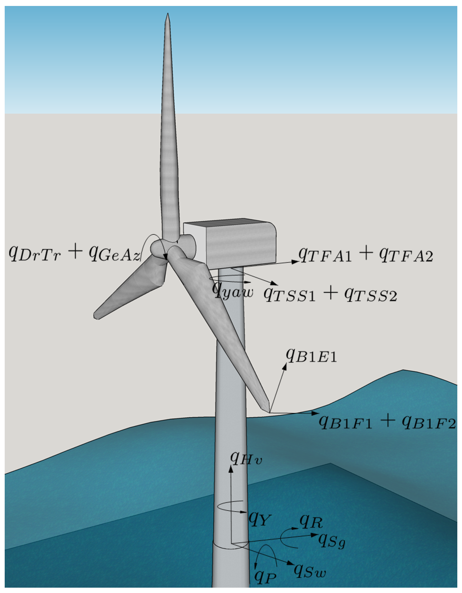
The wind turbine is modelled as a flexible multi-body dynamical system. The various components of importance are the tower, the nacelle, the generator, the gearbox, the low-speed shaft, the hub, and the blades. The tower, the blades, and the low-speed shaft are the flexible components of the wind turbine. Modal analysis is often used to study the dynamics of flexible members. The tower is modelled using the first and second modes in fore-aft and side-to-side directions. Futhermore, the first two modes in flapwise and the first mode in edgewise directions are used for the blades. It is assumed that since the members are highly flexible, the first few modes will capture the dynamics with sufficient accuracy [36]. The degrees of freedom that define the motion of a floating offshore wind turbine are the platform motions, the tower vibrations, the nacelle yaw motion, the torsional distortion of the low-speed shaft, the generator azimuth angle, and the elastic deflections of the three blades. Therefore, the degrees of freedom for a three-bladed wind turbine can be written as

$$\begin{array}{cc}\hfill \mathit{q}=& [q_{Sg}{q}_{Sw}{q}_{Hv}{q}_R{q}_P{q}_Y{q}_{TFA1}{q}_{TSS1}{q}_{TFA2}{q}_{TSS2}{q}_{yaw}{q}_{GeAz}{q}_{DrTr}\cdots \hfill \\ \hfill & \cdots q_{B1F1}{q}_{B1E1}{q}_{B1F2}{q}_{B2F1}{q}_{B2E1}{q}_{B2F2}{q}_{B3F1}{q}_{B3E1}{q}_{B3F2}{]}^T\hfill \end{array}$$

(1)

Therefore, a 22 degrees of freedom model will be derived to model the wind turbine. The degrees of freedom are also denoted by numbers 1 to 22 in the same sequence as presented in Equation (1). The degrees of freedom are schematically shown in Figure 1. A list of the DOFs is presented in Appendix A. Throughout the study, the name of the DOF and its corresponding number will be used interchangeably. Coordinate systems will be assigned to each component, and the motion in its local reference frame will be transformed to the global/inertial reference frame. In the following sections, the coordinate systems required for the wind turbine will be defined, followed by the system’s kinematics and, finally, the system’s kinetics, which will be used to derive the equations of motion.

2.2. Coordinate Systems

As mentioned earlier, individual components of the floating offshore wind turbine are modelled in their local reference frames. A combination of small angle approximation (small angle rotation) and Euler angles (Euler rotation) are used to establish transformation relations between the coordinate systems. Three consecutive rotations ${\theta }_1$, ${\theta }_2$ and ${\theta }_3$ about three mutually orthogonal axes (${\widehat{\mathit{X}}}_{\mathbf{1}},{\widehat{\mathit{X}}}_{\mathbf{2}},{\widehat{\mathit{X}}}_{\mathbf{3}}$) result in a set of orthogonal axes (${\widehat{\mathit{x}}}_{\mathbf{1}},{\widehat{\mathit{x}}}_{\mathbf{2}},{\widehat{\mathit{x}}}_{\mathbf{3}}$). This transformation with small angle approximation can be defined as

$$\left(\begin{array}{c}{\widehat{\mathit{x}}}_{\mathbf{1}}\\ {\widehat{\mathit{x}}}_{\mathbf{2}}\\ {\widehat{\mathit{x}}}_{\mathbf{3}}\end{array}\right)\approx \underset{\mathit{T}}{\underbrace{\left[\begin{array}{ccc}1& {\theta }_3& -{\theta }_2\\ -{\theta }_3& 1& {\theta }_1\\ {\theta }_2& -{\theta }_1& 1\end{array}\right]}}\left(\begin{array}{c}{\widehat{\mathit{X}}}_{\mathbf{1}}\\ {\widehat{\mathit{X}}}_{\mathbf{2}}\\ {\widehat{\mathit{X}}}_{\mathbf{3}}\end{array}\right)$$

(2)

The small angle approximation makes the transformation independent of the order of rotation. Here, the approximation sign is used since the transformation matrix $\mathit{T}$ is not orthonormal and hence the resulting set of axes are not orthogonal to each other. The nearest orthonormal matrix is hence obtained by Singular Value Decomposition (SVD). The nearest orthonormal matrix in Frobenius norm sense ${\mathit{T}}_{\mathit{O}}$ is given as

$${\mathit{T}}_{\mathit{O}}={\mathit{UV}}^{\prime }$$

(3)

where the columns of $\mathit{U}$ contain the eigenvectors of ${\mathit{TT}}^{\prime }$ and the columns of $\mathit{V}$ contain eigenvectors of ${\mathit{T}}^{\prime }\mathit{T}$. This follows from the result of SVD of $\mathit{T}$ obtained as

$$\mathit{T}=\mathit{U}\mathsf{\Sigma }{\mathit{V}}^{\prime }$$

(4)

where $\mathsf{\Sigma }$ is a diagonal matrix containing the singular values of $\mathit{T}$. $\mathsf{\Sigma }$ can be obtained as

$$\mathsf{\Sigma }=\sqrt{\mathrm{eigenvalues}\mathrm{of}{\mathit{TT}}^{\prime }}=\sqrt{\mathrm{eigenvalues}\mathrm{of}{\mathit{T}}^{\prime }\mathit{T}}$$

(5)

The matrix ${\mathit{T}}_{\mathit{O}}({\theta }_1,{\theta }_2,{\theta }_3)$ will be used to define transformations about three mutually perpendicular axes (${\widehat{\mathit{X}}}_{\mathbf{1}},{\widehat{\mathit{X}}}_{\mathbf{2}},{\widehat{\mathit{X}}}_{\mathbf{3}}$) when small angle approximation is employed. The different coordinate systems used are defined as follows.

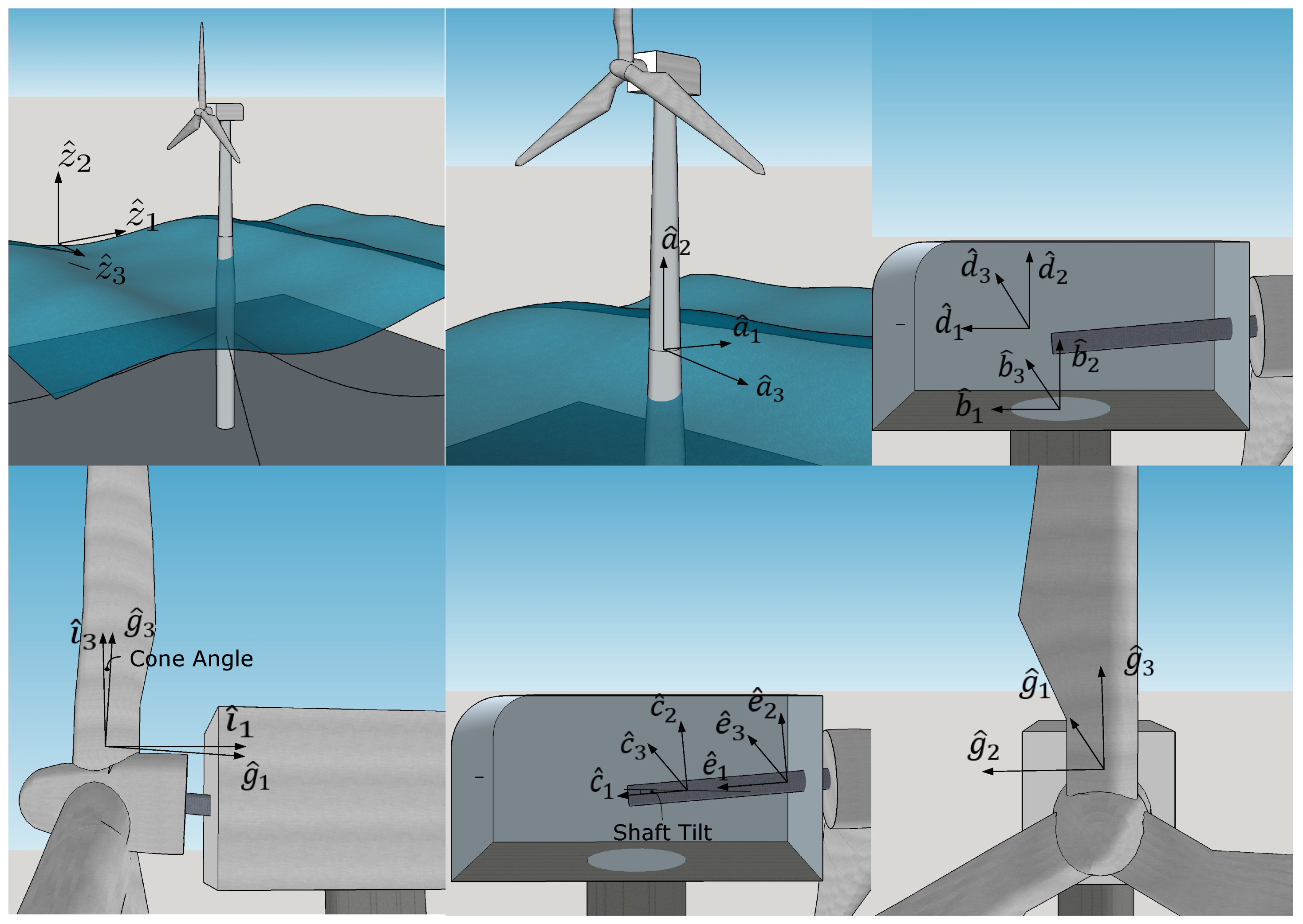
To accurately model a multi-body system like an offshore wind turbine, the kinematics of each sub-component of the wind turbine is first written in its local reference frame and then referred back to the inertial (global) reference frame denoted by $\widehat{\mathit{z}}$. Figure 2 shows the different reference frames used in this paper. As shown in Figure 2, local coordinate systems/reference frames are attached to the floating platform ($\widehat{\mathit{a}}$), tower nodes along the height of the tower, the tower-top ($\widehat{\mathit{b}}$), the nacelle ($\widehat{\mathit{d}}$), non-rotating reference frame attached to the low-speed shaft ($\widehat{\mathit{c}}$) and rotating reference frame ($\widehat{\mathit{e}}$) of the rotor and the blades ($\widehat{\mathit{g}}$). To accurately model the blades, they are first coned ($\widehat{\mathit{i}}$) then pitched (not pictured in Figure 2). Node-fixed coordinate systems are defined on the blades which are further rotated according to the elastic deflection of the blades in out-of-plane and in-plane directions. These blade node-fixed reference frames are used to estimate and return aerodynamic loads. The platform and the blades and the tower deforms/rotates simultaneously about more than one axis. Therefore, Euler rotation matrix cannot be used to define the transformation between two reference frames. However, as the magnitude of these angles is relatively small, the approximation derived in Equation (3) is used. All coordinate systems used in this paper are described in details in Appendix B.

2.3. Kinematics

With all the required coordinate systems on the FOWT defined, the next step is to define the kinematics of the FOWT. For that, first important points on the turbine are identified that describe the kinematics of the entire system. The important points that describe the motion are as follows: Z (tower-base), T (tower node), O (tower-top/base-plate/yaw bearing mass centre), U (nacelle centre of mass), Q (apex of conning angle), C (hub centre of mass), S1 (blade nodes for blade 1), S2 (blade nodes for blade 2) and S3 (blade nodes for blade 3). The various reference frames of importance are denoted as: E (earth/inertial), X (tower base), F (tower body element), B (tower-top/base-plate), N (nacelle), L (low speed shaft on rotor end), M1 (blade 1 element body), M2 (blade 2 element body), M3 (blade 3 element body) and G (high speed shaft/generator).

The complete kinematic description involves defining the position, velocity and acceleration of each rigid and flexible member of the turbine. For brevity, all equations are presented in Appendix B. With the kinematics of the system defined, the kinetics and equations of the motion of the FOWT can be derived as presented in the next section.

2.4. Kinetics and Kane’s Equation of Motion

In this section, the equations of motion of a 3-bladed floating offshore wind turbine will be derived. As per [27], Kane’s equations of motion for a holonomic system with 22 DOFs are stated as

$$F_r+F_r^{\ast }=0\mathrm{for}r=1\mathrm{to}22$$

(6)

where $F_r$ and $F_r^{\ast }$ are the generalised active and the generalised inertia forces respectively. In a set of n rigid bodies characterised by reference frame $N_i$ and centre of mass point $X_i$ the generalised active and inertial forces are given as

$$\begin{array}{cc}\hfill F_r& =\sum _{i=1}^n{}^{\mathit{E}}{\mathit{v}}_{\mathit{r}}^{{\mathit{X}}_{\mathit{i}}}·{\mathit{F}}^{\mathit{i}}+{}^{\mathit{E}}{\mathit{\omega }}_{\mathit{r}}^{{\mathit{N}}_{\mathit{i}}}·{\mathit{M}}^{{\mathit{N}}_{\mathit{i}}}\mathrm{for}r=1\mathrm{to}22\hfill \\ \hfill F_r^{\ast }& =-\sum _{i=1}^n{}^{\mathit{E}}{\mathit{v}}_{\mathit{r}}^{{\mathit{X}}_{\mathit{i}}} · \left(m^{N_i}{}^{\mathit{E}}{\mathit{a}}^{{\mathit{X}}_{\mathit{i}}}\right) - {}^{\mathit{E}}{\mathit{\omega }}_{\mathit{r}}^{{\mathit{N}}_{\mathit{i}}}·{}^{\mathit{E}}{\dot{\mathit{H}}}^{{\mathit{N}}_{\mathit{i}}}\mathrm{for}r=1\mathrm{to}22\hfill \end{array}$$

(7)

At every rigid body $N_i$, the active forces are applied at the centre of mass $X_i$. The time derivative of the angular momentum of rigid body $N_i$ about its centre of mass $X_i$ is obtained as [27]

$${}^{\mathit{E}}{\dot{\mathit{H}}}^{{\mathit{N}}_{\mathit{i}}}=\overline{\overline{\mathit{I}}}{}^{{\mathit{N}}_{\mathit{i}}}·{}^{\mathit{E}}{\mathit{\alpha }}^{{\mathit{N}}_{\mathit{i}}}+{}^{\mathit{E}}{\mathit{\omega }}^{{\mathit{N}}_{\mathit{i}}}\times \overline{\overline{\mathit{I}}}{}^{{\mathit{N}}_{\mathit{i}}}·{}^{\mathit{E}}{\mathit{\omega }}^{{\mathit{N}}_{\mathit{i}}}$$

(8)

The mass of the platform, the tower, the yaw bearing, the nacelle, the hub, the blades and the generator contribute to the total generalised inertia force

$$F_r^{\ast }=F_r^{\ast }{|}_X+F_r^{\ast }{|}_T+F_r^{\ast }{|}_N+F_r^{\ast }{|}_H+F_r^{\ast }{|}_{B1}+F_r^{\ast }{|}_{B2}+F_r^{\ast }{|}_{B3}+F_r^{\ast }{|}_G$$

(9)

Generalised active forces are the forces applied directly on the wind turbine system, constraint forces (springs/links) between the various rigid bodies and internal elastic forces within flexible members. The forces that are applied directly on the offshore wind turbine system include the hydrostatic, hydrodynamic and mooring forces on the floating platform, the aerodynamic forces acting on the blades and the tower and the gravitational forces acting on the entire wind turbine etc. It must be noted here that the gear box friction forces are neglected in this paper. Yaw springs and damper act as constraint forces between the tower and the nacelle. Elasticity of the tower, the blades and the low-speed shaft also contribute to the generalised active forces. Thus the total generalised active force can be given as

$$\begin{array}{cc}\hfill F_r& =F_r{|}_{HydroX}+F_r{|}_{AeroT}+F_r{|}_{AeroB1}+F_r{|}_{AeroB2}+F_r{|}_{AeroB3}+F_r{|}_{GravX}+F_r{|}_{GravT}\hfill \\ \hfill & + F_r{|}_{GravN}+F_r{|}_{GravH}+F_r{|}_{GravB1}+F_r{|}_{GravB2}+F_r{|}_{GravB3}+F_r{|}_{YawSprng}\hfill \\ \hfill & + F_r{|}_{YawDamp}+F_r{|}_{Gen}+F_r{|}_{Brake}+F_r{|}_{ElasticT}+F_r{|}_{ElasticB1}+F_r{|}_{ElasticB2}\hfill \\ \hfill & + F_r{|}_{ElasticB3}+F_r{|}_{DampT}+F_r{|}_{DampB1}+F_r{|}_{DampB2}+F_r{|}_{DampB3}+F_r{|}_{ElasticDrive}\hfill \\ \hfill & + F_r{|}_{DampDrive}\hfill \end{array}$$

(10)

Kane’s equations of motion can be written in matrix form as

$$\mathbf{M}(\mathbf{q},t)\ddot{\mathbf{q}}+\mathbf{f}(\dot{\mathbf{q}},\mathbf{q},t)=0\Rightarrow \mathbf{M}(\mathbf{q},t)\ddot{\mathbf{q}}=-\mathbf{f}(\dot{\mathbf{q}},\mathbf{q},t)$$

(11)

The above equation can be readily solved by a computer using any numerical time integration scheme. This study recommends the use of Runga–Kutta 4$\mathrm{th}$ order method or the Adams-Bashforth-Moulton 4$\mathrm{th}$ order predictor–corrector method. The kinetic description of each individual component is provided in Appendix C.

2.5. Wave–Current Interaction Model

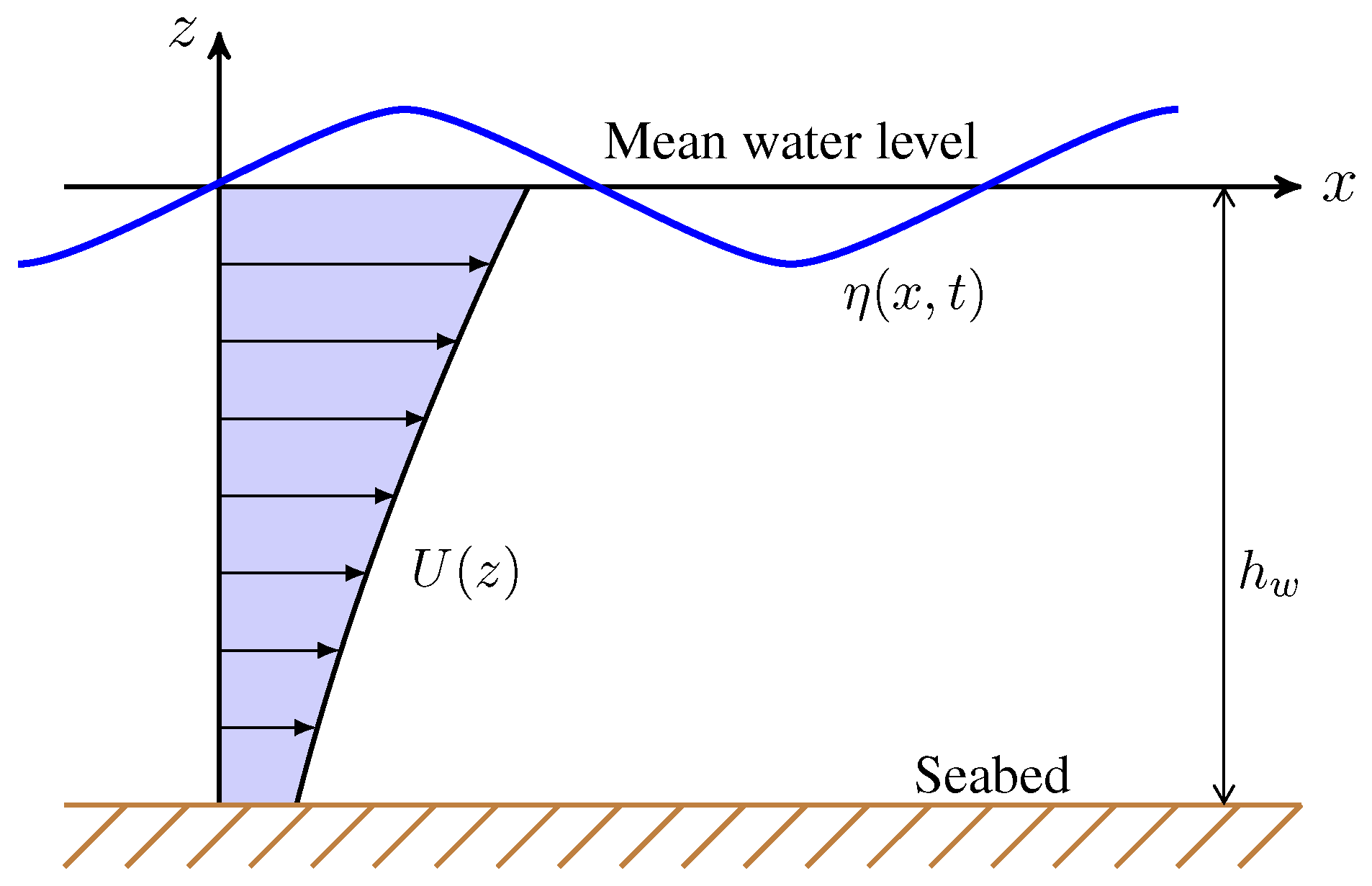
Airy wave theory is used to model the wave–current interaction considering the effect of an underlying current [37,38]. Two-dimensional flow is considered, i.e., waves travelling in a favourable and adverse direction to the underlying current. To describe the flow-field, a coordinate system is established with its origin placed on the mean water level (MWL) with the x-axis denoting the horizontal axis and the z-axis denoting the vertical axis pointing upwards as shown in Figure 3. In Figure 3, $\eta (x,t)$ denotes the time-varying water surface elevation and $U\left(z\right)$ denotes the current velocity profile as a function of z without waves. The still water depth is denoted by $h_w$.

2.5.1. Regular Wave on Current

When the waves travelling on an underlying current has relatively small amplitudes, the velocity field can be expressed as the summation of the flow due to the current and surface wave as [39,40]

$$\begin{array}{cc}\hfill u_T(x,z,t)& =U\left(z\right)+u\left(z\right)cos(\kappa x-\omega t)\hfill \end{array}$$

(12)

$$\begin{array}{cc}\hfill w_T(x,z,t)& =w\left(z\right)sin(\kappa x-\omega t)\hfill \end{array}$$

(13)

where $U\left(z\right)$ is the current velocity as a function of z; $\omega$ and $\kappa$ are the angular frequency and the wave number respectively. It must be noted that $\omega$ is the apparent frequency considering the effect of the underlying current [41]. In the above equations, $u_T(x,z,t)$ and $w_T(x,z,t)$ are the flow velocities in the horizontal and the vertical directions respectively, and $u(x,z,t)$ and $w(x,z,t)$ are the wave velocities using the first-order term [39] in the horizontal and the vertical directions respectively. Using the Airy wave theory, the free surface wave elevation $\eta$ is obtained as

$$\eta (x,t)=Acos(\kappa x-\omega t)$$

(14)

where $A=$ is the amplitude of the surface wave. For a given free surface function and a uniform or linear current profile, the flow velocity can be solved analytically (${\mathrm{d}}^{2}U\left(z\right)/\mathrm{d}{z}^2=0$) (see [40] for details), as

$$\begin{array}{cc}\hfill u_T(x,z,t)=& U\left(z\right)+A(\omega -\kappa U_0)\frac{cosh\left[\kappa (z+h_w)\right]}{sinh\left(\kappa h_w\right)}cos(\kappa x-\omega t)\hfill \end{array}$$

(15)

$$\begin{array}{cc}\hfill w_T(x,z,t)=& A(\omega -\kappa U_0)\frac{sinh\left[\kappa (z+h_w)\right]}{sinh\left(\kappa h_w\right)}sin(\kappa x-\omega t)\hfill \end{array}$$

(16)

where $U_0=$ the current velocity at $z=0$. Futhermore, the corresponding dispersion relation is

$${(\omega -\kappa U_0)}^2=\left[\mathrm{g}\kappa -(\omega -\kappa U_0)\frac{\mathrm{d}U}{\mathrm{d}z}\right]tanh\left(\kappa h_w\right)$$

(17)

valid for uniform and linear shear currents. The flow field can be determined using Equations (15) and (16) after obtaining the wave numbers by solving Equation (17).

2.5.2. Irregular Waves on Current

To evaluate the effect of the underlying current on irregular waves, the Equations (15) and (16) are combined with a spectral model. The effect of the underlying current on the wave spectrum is modelled as [37]

$$S(\omega ,U)=\frac{4S\left(\omega \right)}{{\left(1+\sqrt{1+4\omega U/\mathrm{g}}\right)}^2\sqrt{1+4\omega U/\mathrm{g}}}$$

(18)

where the expressions $S(\omega ,U)$ and $S\left(\omega \right)$ denote the wave spectra with and without the current respectively. It can be noted that, as $\omega \to$$-\mathrm{g}/4U$, the wave is unable to propagate against the current and the wave breaks. The above equation is valid only for $1+4\omega U/g>0$ when waves are travelling on top of an adverse current. To handle the wave breaking case, refs. [42,43] defined an “equilibrium limit” for deep water as

$$S_{\mathrm{ER}}(\omega ,U)=\frac{A^{\ast }{\mathrm{g}}^2}{{(\omega -kU)}^5}\frac{1}{1+2U(\omega -\kappa U)/\mathrm{g}}$$

(19)

where the equilibrium range is denoted by subscript ER and $A^{\ast }$ is a constant between 0.008 and 0.015 [44]. During wave breaking, Equation (19) is used instead for a wave frequency when $S(\omega ,U)$ > $S_{\mathrm{ER}}(\omega ,U)$.

Finally, the water surface elevation is expressed as

$$\eta (x,t)=\sum _{j=1}^N{A}_{j}cos(k_{j}x-{\omega }_{j}t+{\varphi }_j)$$

(20)

where ${\varphi }_j$ is a uniformly distributed random phase angle between 0 to $2\pi$ and N denotes the number of wave components. The amplitude of the jth wave is given as $A_j=\sqrt{2S({\omega }_j,U)\mathsf{\Delta }\omega }$ with $\mathsf{\Delta }\omega$ the frequency interval. The corresponding flow velocities are given as

$$\begin{array}{cc}\hfill u_T(x,z,t)=& U\left(z\right)+\sum _{j=1}^N{A}_j({\omega }_j-{\kappa }_{j}U)\frac{cosh\left[{\kappa }_j(z+h_w)\right]}{sinh\left({\kappa }_j{h}_w\right)}cos({\kappa }_{j}x-{\omega }_{j}t+{\varphi }_j)\hfill \end{array}$$

(21)

$$\begin{array}{cc}\hfill w_T(x,z,t)=& \sum _{j=1}^N{A}_j({\omega }_j-{\kappa }_{j}U)\frac{sinh\left[{\kappa }_j(z+h_w)\right]}{sinh\left({\kappa }_j{h}_w\right)}sin({\kappa }_{j}x-{\omega }_{j}t+{\varphi }_j)\hfill \end{array}$$

(22)

The accelerations can be obtained from the preceding equations, as

$$\begin{array}{cc}\hfill {\dot{u}}_T(x,z,t)=& \sum _{j=1}^N{A}_j{\omega }_j({\omega }_j-{\kappa }_{j}U)\frac{cosh\left[{\kappa }_j(z+h_w)\right]}{sinh\left({\kappa }_j{h}_w\right)}sin({\kappa }_{j}x-{\omega }_{j}t+{\varphi }_j)\hfill \end{array}$$

(23)

$$\begin{array}{cc}\hfill {\dot{w}}_T(x,z,t)=& -\sum _{j=1}^N{A}_j{\omega }_j({\omega }_j-{\kappa }_{j}U)\frac{sinh\left[{\kappa }_j(z+h_w)\right]}{sinh\left(k_j{h}_w\right)}cos({\kappa }_{j}x-{\omega }_{j}t+{\varphi }_j)\hfill \end{array}$$

(24)

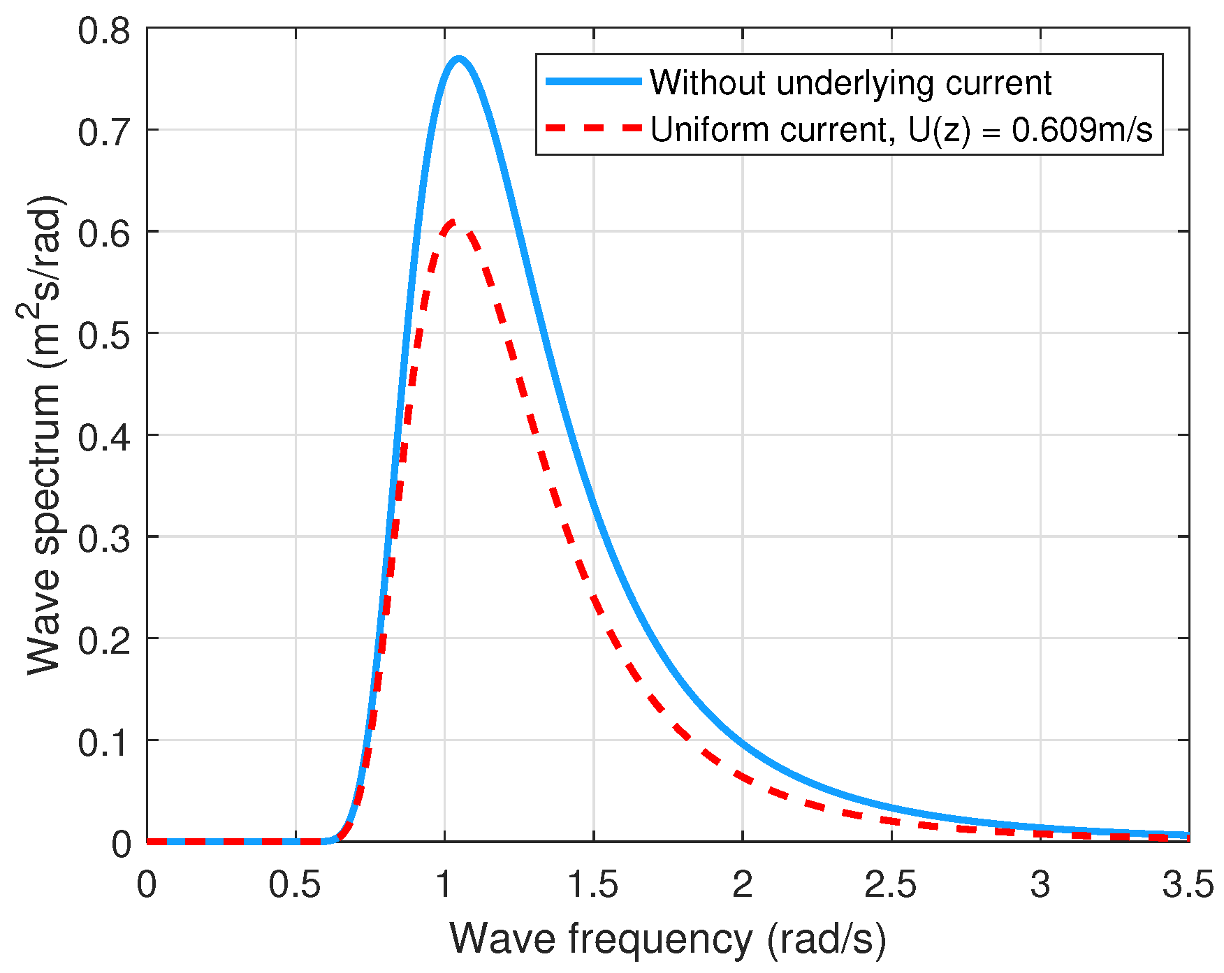
where the wave-number ${\kappa }_j$ is obtained by solving Equation (17) for each wave component. Figure 4 presents an example of the Pierson–Moskowitz spectrum with and without an underlying linear current. The significant wave height is 3 m, the peak spectral period is 6 s and surface current velocity of the underlying uniform current profile is 0.609 m/s [45]. It can be observed that there is a reduction of the wave spectrum peak in the presence of an underlying current.

2.6. Aerodynamic Loads

The popular Blade Element Momentum (BEM) theory is used in this paper to estimate the aerodynamic loads on the wind turbine. The TurbSim [46] package is used to create the 3D wind fields. TurbSim [46] generated wind fields account for spatial coherence of the turbulence along with vertical and horizontal wind shear. The package takes the characteristic wind speeds at a reference height, turbulence intensity level, and wind power-law coefficients for wind shear as some of the primary inputs. The BEM program used in this paper interpolates the wind speeds at the blade nodes from the TurbSim wind fields. It estimates aerodynamic loads using the blades’ quasi-static aerodynamic properties (i.e., lift and drag). The BEM theory is widely available in the literature [47,48,49] and is not repeated here.

A new solution approach proposed by Ning [50] was used here to solve the BEM equations. In this approach, a 1D root finding method (fzero in MATLAB) is to find the unknown inflow angle instead of solving the three-dimensional problem of finding the tangential and the axial induction factors. Different equations are used in the momentum, empirical, and propeller brake region to form the solution in this approach. Furthermore, the empirical region is modified using Glauert’s correction with Buhl’s modification. As described by [50], using different equations for the different regions enables us to circumvent the traditional two-point iterative procedure of solving the BEM equations. To account for the vortices generated by the blade tips and the hub, Prandtl’s hub, and tip loss correction factors are also included in the program. The Pitt and Peters correction for skewed inflow has also been included in the program. The solution of the BEM equations at a radial distance r gives the lift and drag forces on the blades a radial distance r from the root of the blade. The out-of-plane force (thrust) and in-plane force (torque) on the blades is then estimated from the lift and drag forces. These forces are then integrated along the length of the blades to obtain the total forces on the blades. For details on the procedure, please refer to [51].

2.7. Hydrodynamic Loads

The hydrodynamic loads on the cylindrical spar of the wind turbine is estimated using Morison’s equation. Morison’s equations together with strip theory is used to estimate the linear wave inertia forces and the non-linear viscous drag forces. The total wave loads on the platform is estimated by integrating the elemental forces along the length/depth of the platform. The hydrodynamic forces on a strip $\mathrm{d}z$ of the platform in surge and sway directions respectively are given as

$$\begin{array}{cc}\hfill \mathrm{d}{F}_i^P(z,t)=& \underset{\mathrm{added}\mathrm{mass}}{\underbrace{-C_A\rho \left(\frac{\pi D{\left(z\right)}^2}{4}\right){\ddot{q}}_i(z,t)\mathrm{d}z}}+\underset{\mathrm{fluid}\mathrm{inertial}\mathrm{force}}{\underbrace{C_M\rho \left(\frac{\pi D{\left(z\right)}^2}{4}\right)a_i^f(z,t)\mathrm{d}z}}\hfill \\ \hfill & + \underset{\mathrm{viscous}\mathrm{drag}\mathrm{force}}{\underbrace{\frac{1}{2}{C}_D\rho D\left(z\right)\left(v_i^f(z,t)-v_i^p(z,t)\right)|v_i^f(z,t)-v_i^p(z,t)|\mathrm{d}z}}\hfill \end{array}\mathrm{for}i=Sg,Sw$$

(25)

where $\mathrm{d}{F}_i^P$ is the elemental force on the platform along the $i\mathrm{th}$ degree of freedom. The rolling and pitching moments on the platform can be obtained as

$$\mathrm{d}{M}_i^P(z,t)= \left\{\begin{array}{cc}-\mathrm{d}{F}_{Sg}^P(z,t)z\hfill & i=P\hfill \\ \mathrm{d}{F}_{Sw}^P(z,t)z\hfill & i=R\hfill \end{array}\right.$$

(26)

where $\mathrm{d}{M}_i^P$ is the moment per unit length on the platform for the $i\mathrm{th}$ degree of freedom. The total forces and moments on the platform are obtained by integrating the distributed forces and moments along the length/depth of the platform. For the symmetrical spar, the heave force and the yaw moment are assumed to be zero. Morison’s equations assume that viscous drag forces dominate the total drag forces on the platform and the radiation damping is negligible. This assumption is valid when the cylinder diameter is small compared to the wavelength and the platform’s small motion. It must be noted that Equation (25) does not include the added mass associated with the platform heave degree of freedom. Hence, added mass coefficient as per [18] is included in this paper for the heave degree of freedom.

2.8. Mooring Dynamics Model

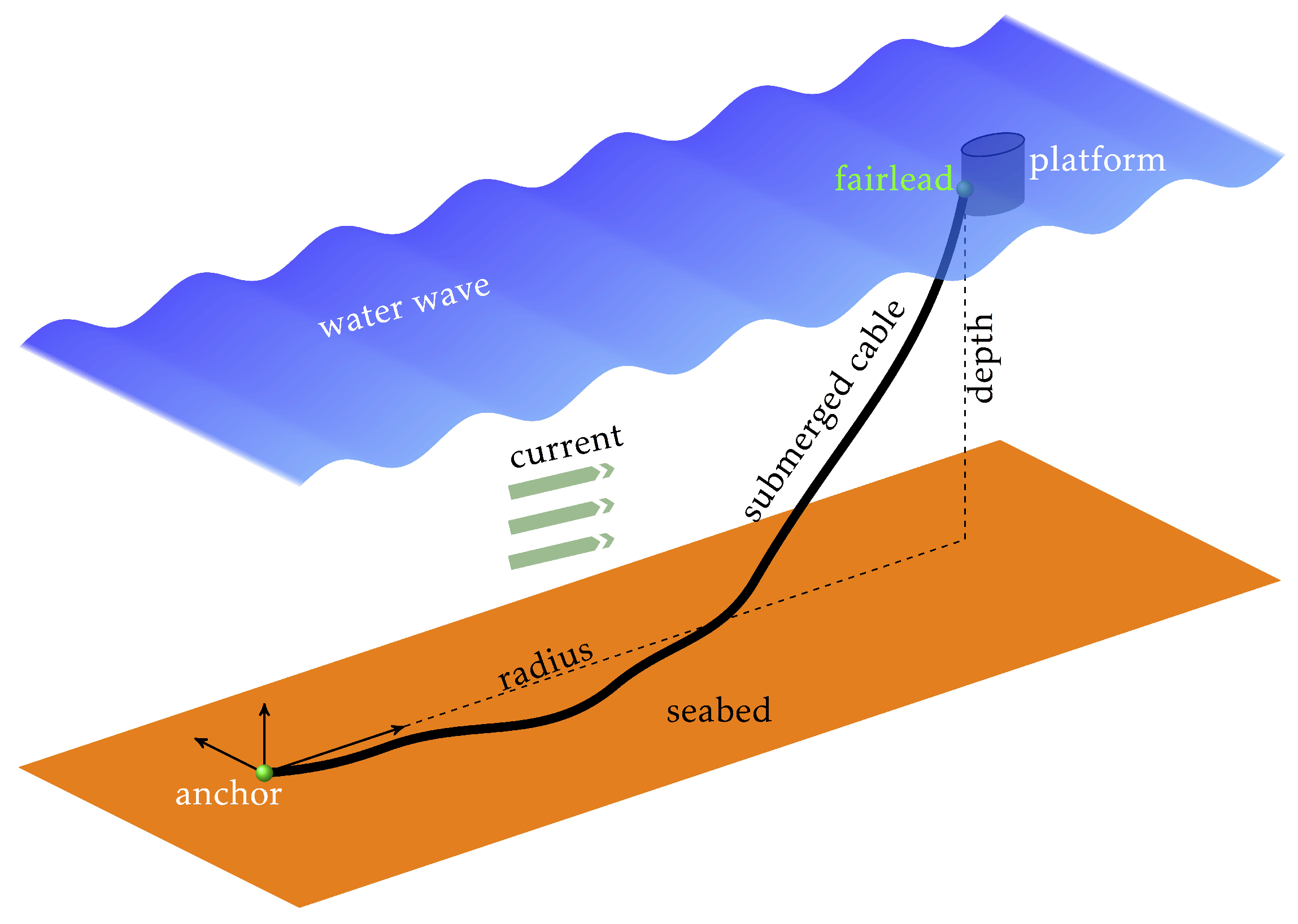
OpenMOOR [52] is used to estimate the mooring force on the platform in this paper. OpenMOOR is an open-source mooring system simulation program developed by L Chen et al. [52] that can be used to estimate the mooring forces at a reference point on a platform. The program is developed based on the model of submerged cables [53,54,55], as shown in Figure 5. The cables are modelled as Euler beams, including the effects of its bending and torsional stiffness. The hydrodynamic forces are included using the modified Morison’s equations. For the part of the cable grounded on the seabed, the seabed is modelled as a flat visco-elastic mattress. The seabed stiffness was obtained from the FAST [25] case files. The cable fairlead forces and consequently the FOWT motion are not sensitive to the value of the seabed stiffness as reported in the literature and verified here using a parametric analysis. However, it must be noted that the seabed stiffness is important in case of fatigue analysis of the cable near the touchdown point. When using OpenMOOR to solve for the mooring forces, the fairlead motion is first computed using the multi-body dynamics (in this case, the wind turbine). Then the two-point boundary problem for all three cables is solved parallelly using the generalised-$\alpha$ method for both spatial and temporal discretization [55]. A Newton-like method with dynamic relaxation is used to solve the resulting non-linear algebraic equation. OpenMOOR is also capable of including steady ocean currents of arbitrary profiles. In this paper, the effect of waves on the mooring cable is ignored as the fairleads of the turbine are deep below the mean water level (MWL), where currents are predominant. In this work, OpenMOOR is separately compiled into a dynamic linking library and imported/coupled with the multi-body dynamic model of the FOWT in MATLAB^®.

The multi-body code of the FOWT is coupled with OpenMoor. The displacements and velocities of the platform reference points are sent to OpenMoor, and the estimated mooring loads are applied on the platform. This soft-coupling creates a one-time step time lag between the platform/wind turbine state and OpenMoor loads. However, the error becomes insignificant with a sufficiently small time step, and this requirement can be waived. A similar practice can be found in state-of-the-art simulation tools like FAST [25].

2.9. Structural Control—Passive TMDI Installed on Tower-Top

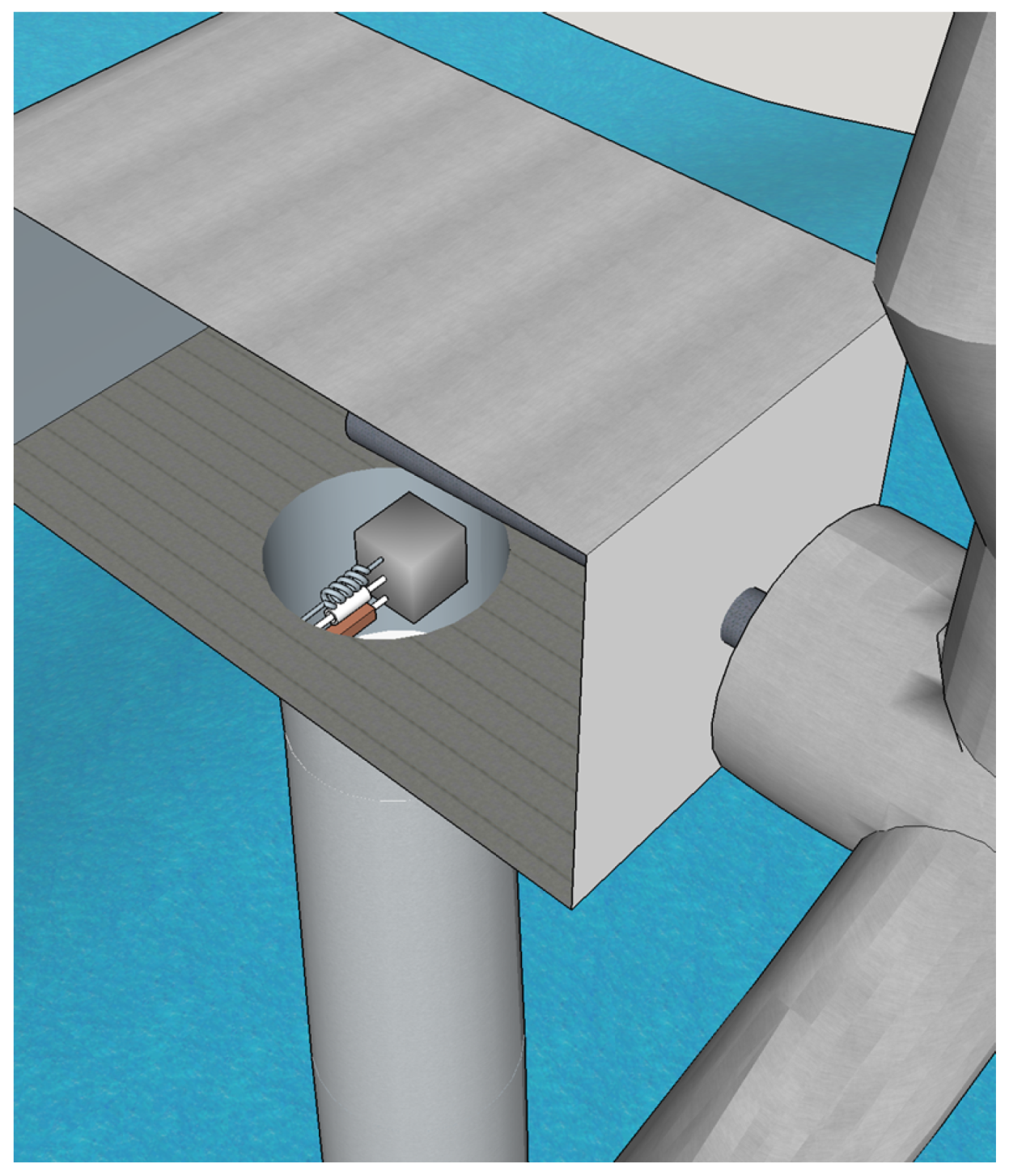
In this section a passive Tuned Mass Damper Inerter (TMDI) is installed inside the top of the tower to mitigate vibrations of the wind turbine tower. The damper is installed in the tower as shown in Figure 6.

The TMDI is a relatively new concept in which an ‘inerter’ device (mechanical flywheel-based device in this case) is attached in parallel to the linear spring and the linear damper to the mass of a classical tuned mass damper (TMD). The inerter transforms the linear translation of the tuned mass into a rotation of the flywheels to provide a mass amplification effect on the classical TMD. The mass amplification effect increases the device’s vibration control capabilities, enabling one to achieve enhanced vibration control using a relatively lighter damper. Several recent studies have investigated the use of TMDIs for vibration control of FOWTs [31,56,57]. This section will demonstrate the procedure of installing a TMDI device inside a FOWT using Kane’s method and will emphasise the relative ease of the procedure compared to traditional energy formulation-based methods.

Installing a TMDI in the tower is straightforward because the position of the essential points on the wind turbine is not dependent on the position of the TMDI mass. The position of the TMDI mass is denoted by the new generalised coordinate $q_{TMDI}$ which is also denoted by the number 23. Therefore, the position vectors, velocity vectors, etc. derived previously do not change. Only the position vector of the TMDI mass needs to be derived, followed by its partial linear velocities and acceleration. The kinematic and kinetic description of the TMDI placed on top of the tower is provided in Appendix D. The resulting system matrices of the TMDI superimposed on the overall system matrices result in the coupled system matrices of the FOWT-TMDI system.

2.9.1. TMDI Parameter Optimization Using a Simplified Model

The floating offshore wind turbine system coupled with a TMDI system has a complicated set of non-linear equations of motion that cannot optimise the TMDI properties in closed form. Therefore, to derive the optimal properties of the TMDI, a couple of simplifications have been made

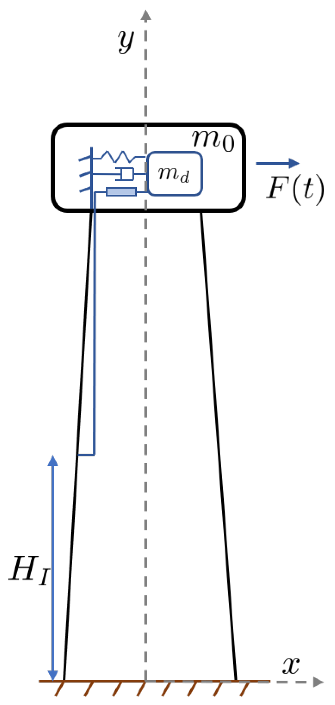
• A 2-DOF system with the TMDI represents the wind turbine placed on top of the tower as shown in Figure 7.
• The wind turbine is subjected to white noise.
• The mass of the blades, the hub, and the nacelle are lumped on top of the tower and its base is fixed.
• The inerter is hooked between the mass of the damper and the tower at an arbitrary height $H_I$ from the base of the tower.
• The primary structure, in this case, the wind turbine tower, does not offer any damping.

Under the above assumptions, the governing equations of motion normalised by the mass of the primary structure $m_0$ is given as

$$\begin{array}{cc}\hfill \left[\begin{array}{cc}1+\mu +\beta {(1-\varphi )}^2& \mu +\beta (1-\varphi )\\ \mu +\beta (1-\varphi )& \mu +\beta \end{array}\right]\left(\begin{array}{c}{\ddot{q}}_t\\ {\ddot{q}}_d\end{array}\right)& + \left[\begin{array}{cc}0& 0\\ 0& 2\mu {\omega }_t{\zeta }_d{\omega }_r\end{array}\right]\left(\begin{array}{c}{\dot{q}}_t\\ {\dot{q}}_d\end{array}\right)\hfill \\ & + \left[\begin{array}{cc}{\omega }_t^2& 0\\ 0& \mu {\omega }_t^2{\omega }_r^2\end{array}\right]\left(\begin{array}{c}{q}_t\\ q_d\end{array}\right)=\left(\begin{array}{c}\frac{F}{m_0}\\ 0\end{array}\right)\hfill \end{array}$$

(27)

$q_t$ and $q_d$ denotes the tower and the damper degrees of freedom respectively. $\mu$ is the mass ratio and $\beta$ is the inerter ratio defined as

$$\mu =\frac{m_d}{m_0}\beta =\frac{b}{m_0}$$

(28)

where $m_d$ is the damper mass and b is the inertance [58]. b has the units of mass and details can be found in [58,59]. The tuning ratio and damping ratio of the damper are defined as

$${\omega }_r=\frac{{\omega }_d}{{\omega }_t}{\zeta }_d=\frac{c_d}{2m_d{\omega }_d}$$

(29)

where ${\omega }_t$ and ${\omega }_d$ are the natural frequency of the tower and the damper respectively, and $c_d$ is the damping coefficient of the TMDI. The normalised (normalised to 1) displacement of the tower at a height $H_I$ from its base can be obtained directly from the primary mode shape as

$$\varphi ={\varphi }_t\left(H_I\right)\mathrm{where}0\le \varphi \le 1$$

(30)

where ${\varphi }_t$ is the primary mode shape of the tower. F is the white noise excitation force of constant intensity. For such a system the optimum tuning parameters were obtained by [31] as

$${\omega }_r=\sqrt{\frac{-B+\sqrt{B^2-AC}}{2A}}$$

(31)

where

$$\begin{array}{cc}\hfill A& =3{\mu }^2({\mu }^2+2\mu {\varphi }^2\beta -4\mu \varphi \beta +2\mu \beta +2\mu +{\varphi }^4{\beta }^2-4{\varphi }^3{\beta }^2+6{\varphi }^2{\beta }^2+2{\varphi }^2\beta -4\varphi {\beta }^2\hfill \\ \hfill & - 4\varphi \beta +{\beta }^2+2\beta +1)\hfill \\ \hfill B& =\mu (4{\mu }^2{\zeta }_d^2-{\mu }^2+4\mu {\varphi }^2{\zeta }_d^2\beta -2\mu {\varphi }^2\beta -8\mu \varphi {\zeta }_d^2\beta +2\mu \varphi \beta +4\mu {\zeta }_d^2\beta +4\mu {\zeta }_d^2-2\mu \beta \hfill \\ \hfill & - 2\mu -{\varphi }^2{\beta }^2+2\varphi {\beta }^2\hfill \\ \hfill & - {\beta }^2-2\beta )\hfill \\ \hfill C& =-({\mu }^2+2\mu \beta +{\beta }^2)\hfill \end{array}$$

and the optimal damping ratio

$${\zeta }_d=\frac{1}{2\mu {\omega }_r}\sqrt{\frac{D}{E}}$$

(32)

where

$$\begin{array}{cc}\hfill D& ={\mu }^4{\omega }^4+2{\mu }^3{\varphi }^2\beta {\omega }_r^4-4{\mu }^3\varphi \beta {\omega }_r^4+2{\mu }^3\beta {\omega }_r^4+2{\mu }^3{\omega }_r^4-{\mu }^3{\omega }_r^2+{\mu }^2{\varphi }^4{\beta }^2{\omega }_r^4\hfill \\ \hfill & - 4{\mu }^2{\varphi }^3{\beta }^2{\omega }_r^4+6{\mu }^2{\varphi }^2{\beta }^2{\omega }_r^4+2{\mu }^2{\varphi }^2\beta {\omega }_r^4-2{\mu }^2{\varphi }^2\beta {\omega }_r^2-4{\mu }^2\varphi {\beta }^2{\omega }_r^4\hfill \\ \hfill & - 4{\mu }^2\varphi \beta {\omega }_r^4+2{\mu }^2\varphi \beta {\omega }_r^2+{\mu }^2{\beta }^2{\omega }_r^4+2{\mu }^2\beta {\omega }_r^4-2{\mu }^2\beta {\omega }_r^2+{\mu }^2{\omega }_r^4-2{\mu }^2{\omega }_r^2+{\mu }^2\hfill \\ \hfill & - \mu {\varphi }^2{\beta }^2{\omega }_r^2+2\mu \varphi {\beta }^2{\omega }_r^2-\mu {\beta }^2{\omega }_r^2-2\mu \beta {\omega }_r^2+2\mu \beta +{\beta }^2\hfill \\ \hfill E& =\mu +{\varphi }^2\beta -2\varphi \beta +\beta +1\hfill \end{array}$$

Note that Equations (31) and (32) reduce to the optimal tuning parameters for classical TMD(s) when $b=\beta =0$ and the primary structure is excited by white noise. In addition, note that Equations (31) and (32) are coupled. Hence, an iterative procedure must to used with a sufficiently small tolerance to find the optimal parameter. It is found that a simple iterative scheme is capable for finding the solution with sufficient speed and accuracy.

3. Results and Discussion

The previous section detailed the method of deriving the equations of motion of a FOWT and the associated dynamic (aerodynamic and hydrodynamic) loads. To demonstrate the accuracy of the developed dynamic model, the developed model is compared and validated against state-of-the-art wind turbine simulator FAST [25]. The results are provided in the following sub-section. Next, the performance of a optimally tuned TMDI is investigated in the following sub-section.

3.1. Benchmarking against FAST v8

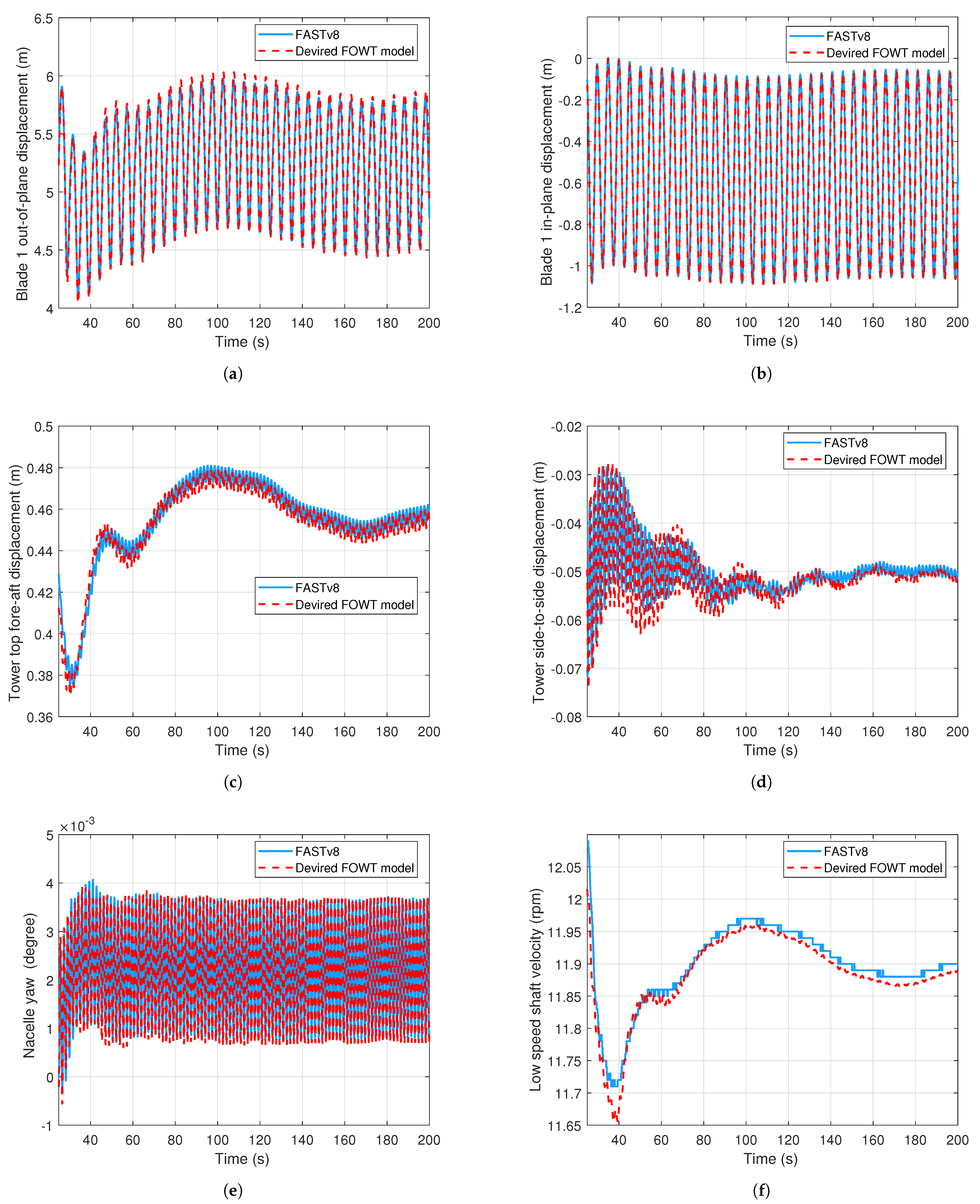
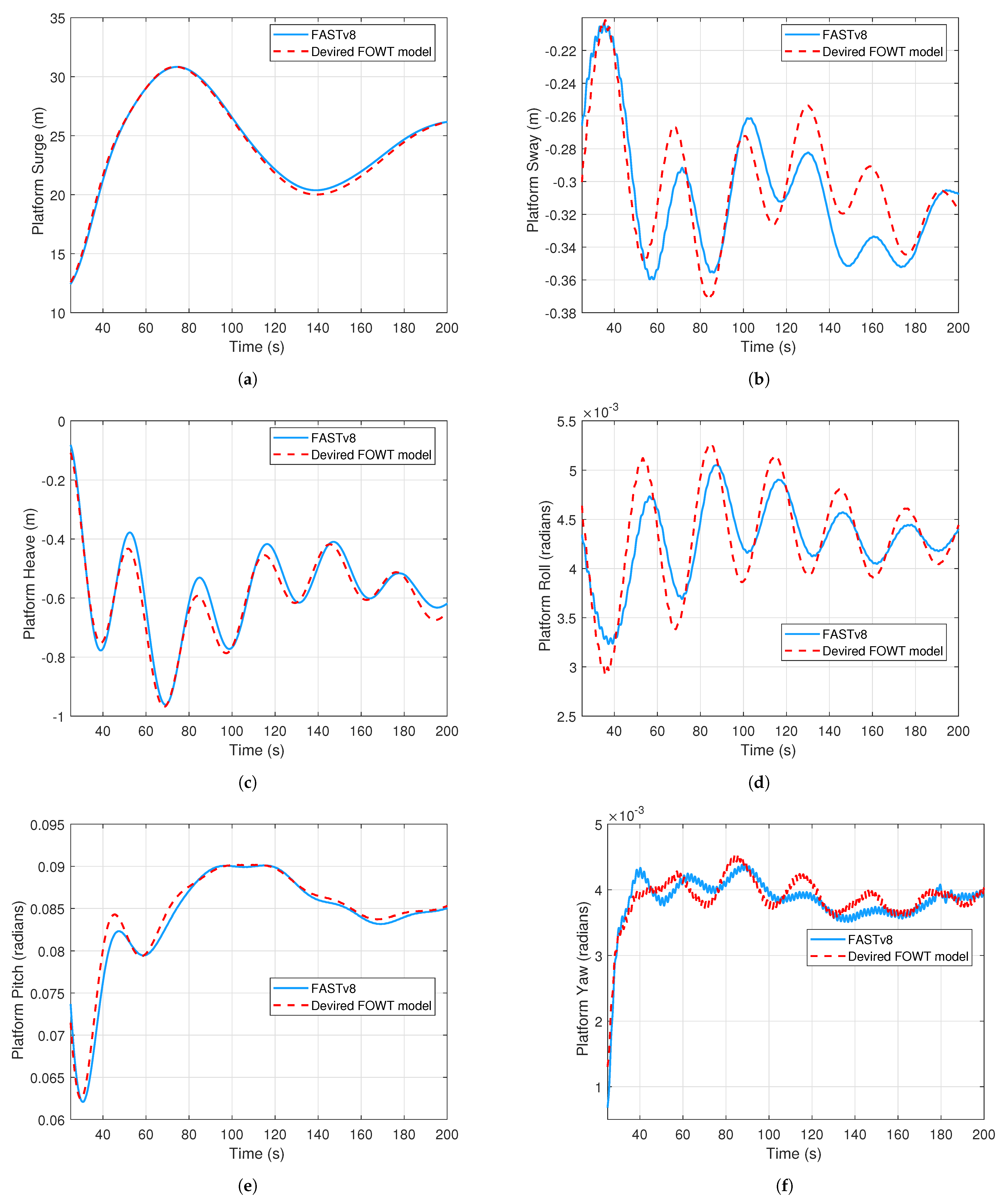
All numerical codes used to model the FOWT are developed in MATLAB^®. In this section, the floating offshore wind turbine model developed in this study is validated against the state-of-the-art wind turbine simulator FAST [25] using code-to-code comparison. The spar type FOWT multi-body dynamic model developed theoretically is instantiated using the details provided from the NREL 5 MW baseline offshore wind turbine [60]. The basic properties of the floating wind turbine are provided in

Table 1. Basic properties of the NREL 5 MW baseline offshore wind turbine.

Baseline turbine properties
Rating	5 MW
Rotor orientation, no of blades	Upwind, 3 blades
Rotor diameter, hub diameter	126 m, 3 m
Hub height	90 m
Cut-in, rated, cut-out wind speeds	3 m/s, 11.4 m/s, 25 m/s
Cut-in, rated rotor speeds	6.9 RPM, 12.1 RPM
Rated tip speed	80 m/s
Control	Variable speed, collective pitch
Drivetrain	3-stage gearbox
Overhang, shaft tilt, precone	5 m, 5${}^{\circ }$, 2.5${}^{\circ }$
Tower properties
Elevation of tower base from SWL	10 m
Elevation of tower top from SWL	87.6 m
Floating platform properties
Depth of platform base below SWL	120 m
Elevation of platform top above SWL	10 m
Depth to top of taper below SWL	4 m
Depth to bottom of taper below SWL	12 m
Platform diameter above taper	6.5 m
Platform diameter below taper	9.4 m

, for more details on the wind turbine, please refer to [60]. The offshore wind turbine is simulated under a steady (rated) wind speed of 11.4 m/s in still water for verification purposes. The aerodynamic loads are calculated using the Blade Element Momentum Theory (BEM), as described previously. The verification results for the primary structural responses are shown in Figure 8. The other responses of the offshore wind turbine are provided in Figure A1 in Appendix F. A comparison of the time histories after the initial transient phase (50 s) is presented in terms of the mean, standard deviation, and max/min values in

Table 2. Comparison of response statistic between FAST and the derived model (DM).

Response	Mean		Min		Max		Std.
	FAST	DM	FAST	DM	FAST	DM	FAST	DM
Blade OOP displacement (m)	5.283	5.296	4.396	4.366	5.971	6.037	0.448	0.477
Blade IP displacement (m)	−0.559	−0.565	−1.085	−1.090	−0.038	−0.046	0.354	0.353
Tower-top FA displacement (m)	0.460	0.458	0.436	0.431	0.481	0.478	0.011	0.011
Tower-top SS displacement (m)	−0.051	−0.051	−0.058	−0.062	−0.040	−0.040	0.003	0.003
Nacelle yaw angle (${}^{\circ }$)	2.2E-3	2.2E-3	7.1E-4	6.1E-4	3.8E-3	3.8E-3	1.0E-3	1.0E-3
Rotor speed (RPM)	11.910	11.899	11.840	11.834	11.970	11.959	0.035	0.035
Platform surge (m)	25.075	24.872	20.380	20.009	30.830	30.837	3.430	3.564
Platform sway (m)	−0.319	−0.309	−0.359	−0.372	−0.261	−0.253	0.026	0.027
Platform heave (m)	−0.589	−0.611	−0.961	−0.968	−0.377	−0.417	0.133	0.131
Platform roll (rad)	4.4E-3	4.4E-3	3.7E-3	3.4E-3	5.1E-3	5.3E-3	2.95E-4	4.45E-4
Platform pitch (rad)	0.085	0.086	0.079	0.079	0.090	0.090	3.1E-3	2.9E-3
Platform yaw (rad)	3.9E-3	3.9E-3	3.5E-3	3.6E-3	4.4E-3	4.5E-3	2.1E-4	2.1E-4

. The numerical results compare satisfactorily with FAST [25] which numerically verifies the developed multi-body model using Kane’s method.

The responses of the floating offshore wind turbine tower, blades, nacelle, and low-speed shaft match very well with the ones obtained from FAST [25] as shown in Figure 8. However, minor dissimilarities are observed in the platform motion in Figure A1. A phase shift can be observed in the floating platform response time histories. While FAST [25] includes radiation forces from the linear potential flow theory together with viscous drag forces from Morison’s equation, the model derived here only includes the viscous drag forces from Morison’s equation. The difference in the resulting hydrodynamic damping forces manifests a phase shift in the response time histories. It is also noteworthy that the degrees of freedom that are subjected to lower levels of hydrodynamic damping like the platform surge, the platform heaves or reaches steady state quickly like platform pitch and the platform yaw is less affected by this phase shift. The degrees of freedom most affected by this phase shift are the platform sway and roll degrees of freedom. However, it can be observed that the mean and the frequency content of all of the responses match very well with FAST [25] which is most important from a dynamic analysis point of view.

3.2. Performance of the Passive TMDI

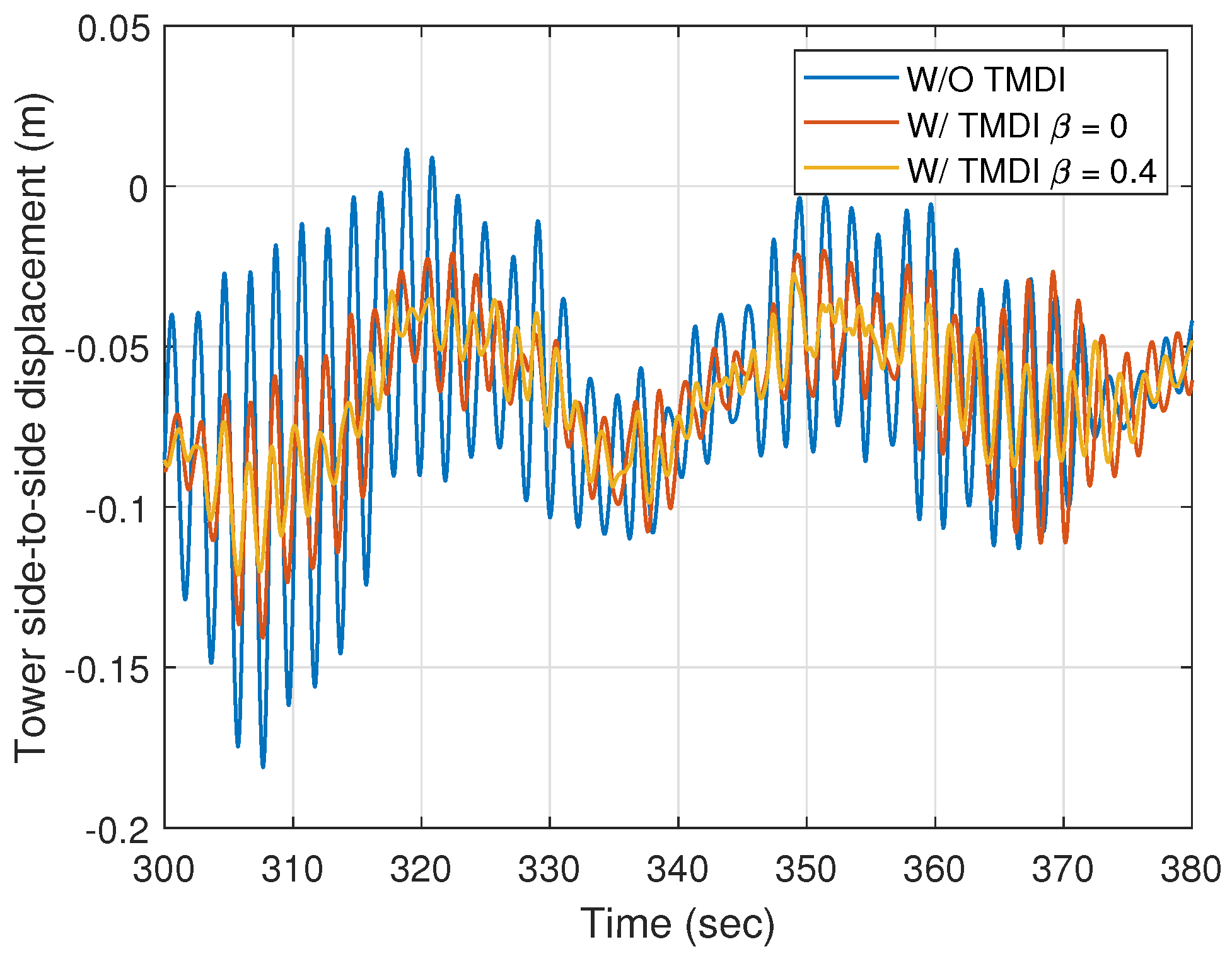
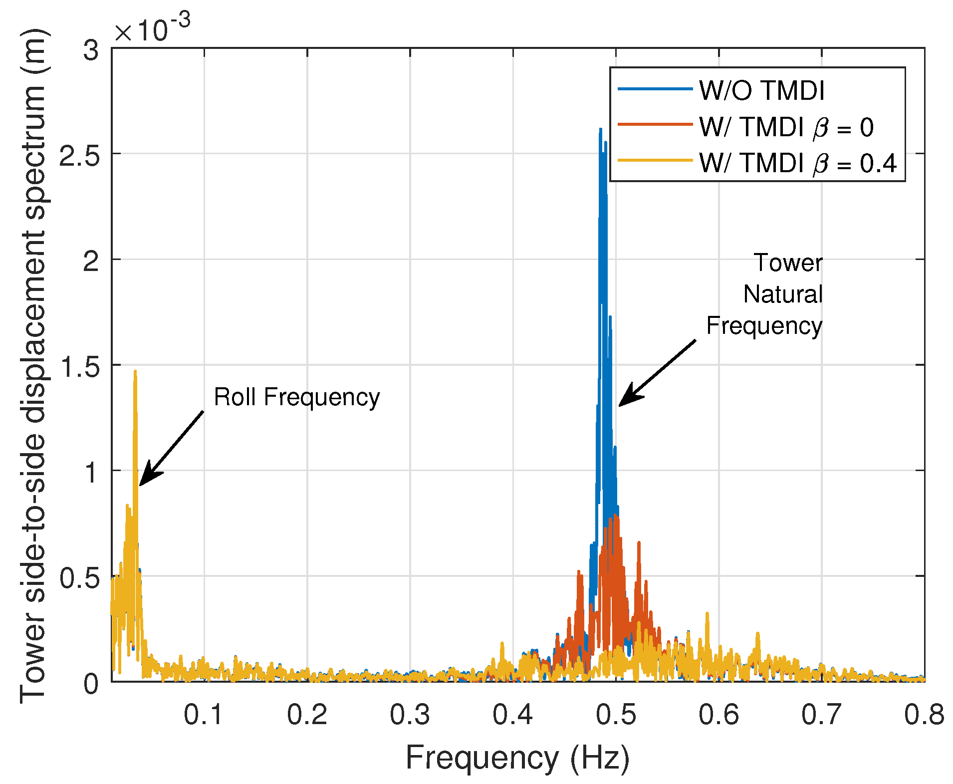
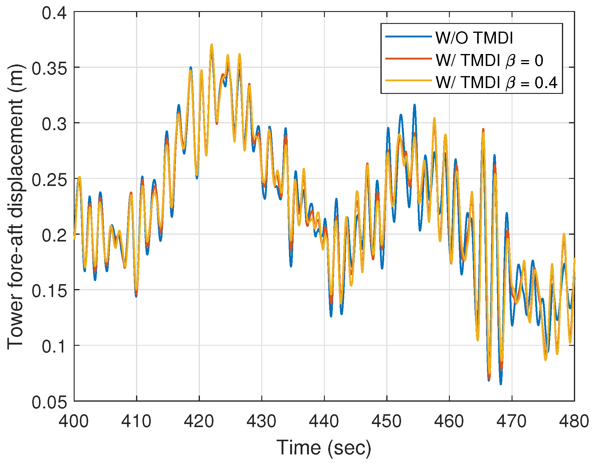
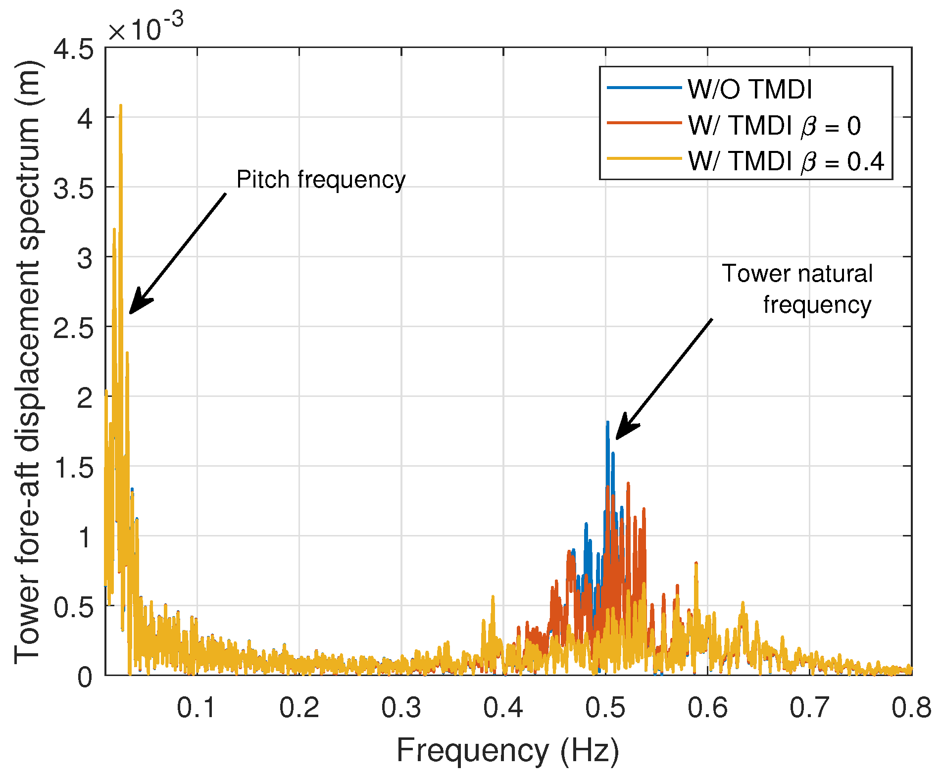
The TMDI is coupled to the baseline offshore wind turbine [60] used earlier in this study. The TMDI is optimised according to Section 2.9.1. The damper’s performance has been investigated over an extensive range of wind-wave loading environments by the authors in [31]. In this paper, only one case of met-ocean condition is presented for illustrative purposes. The chosen met-ocean condition has a hub-height mean wind speed of 20 m/s, a significant wave height of 6 m, and a peak spectral period of 8 s. The TMDI is installed in the nacelle, has 1% of the tower mass (excluding the RNA), and is tuned to the tower’s natural frequency. The tower side-to-side motion with and without the TMDI is shown in Figure 9 and Figure 10. Futhermore, the tower fore-aft motion with and without the TMDI is shown in Figure 11 and Figure 12. Excellent damping of the tower side-to-side vibrations is observed using a damper having a mass of just 1% of the tower mass. On the other hand, the vibration reduction for the fore-aft motion of the tower is modest as the fore-aft modes experience considerable aerodynamic damping. The figures also include a case where the inerter ratio $\beta$ is zero, reducing the TMDI to a classical TMD. It can be observed that, expectantly, the performance of the classical TMD is considerably worse than the TMDI.

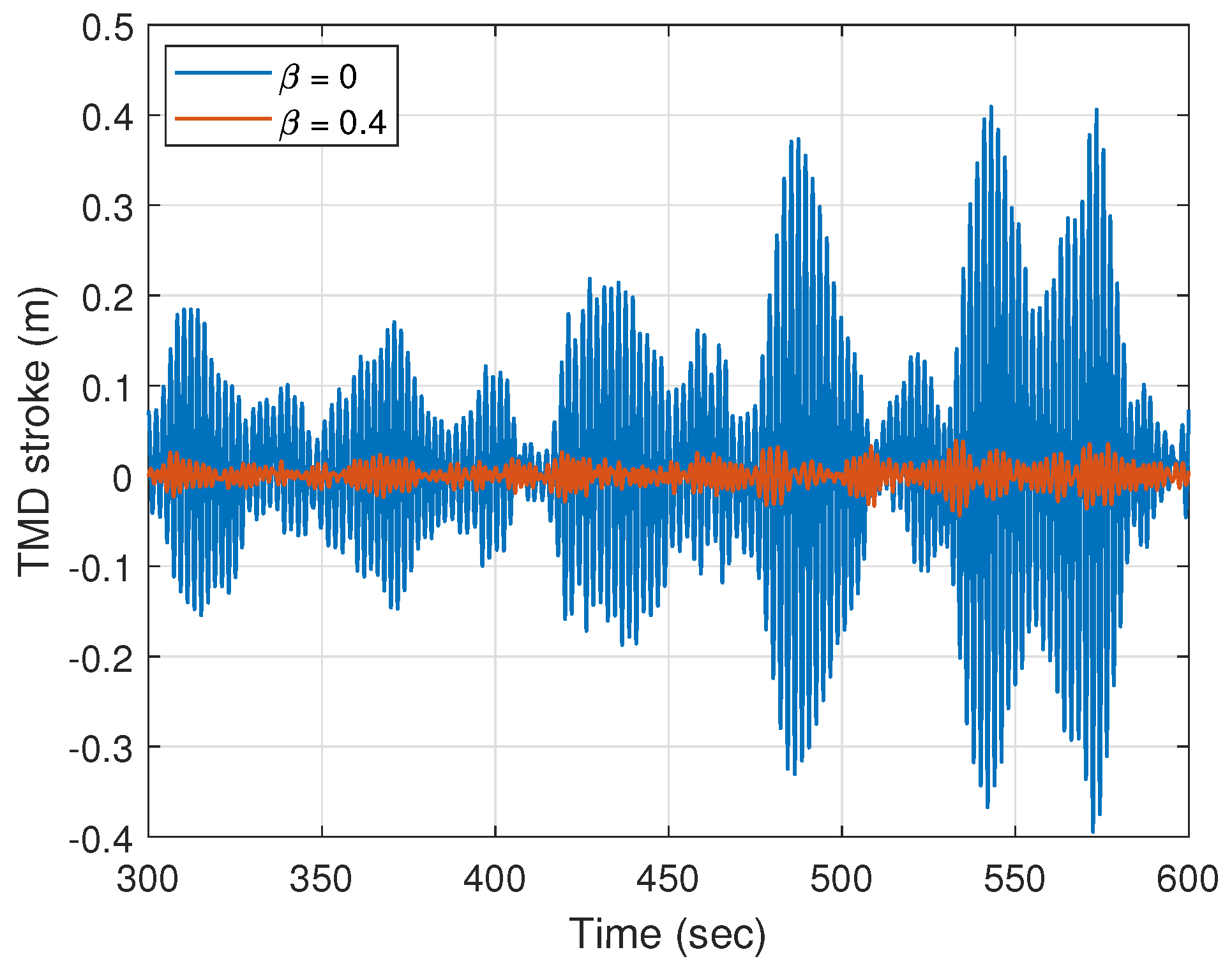
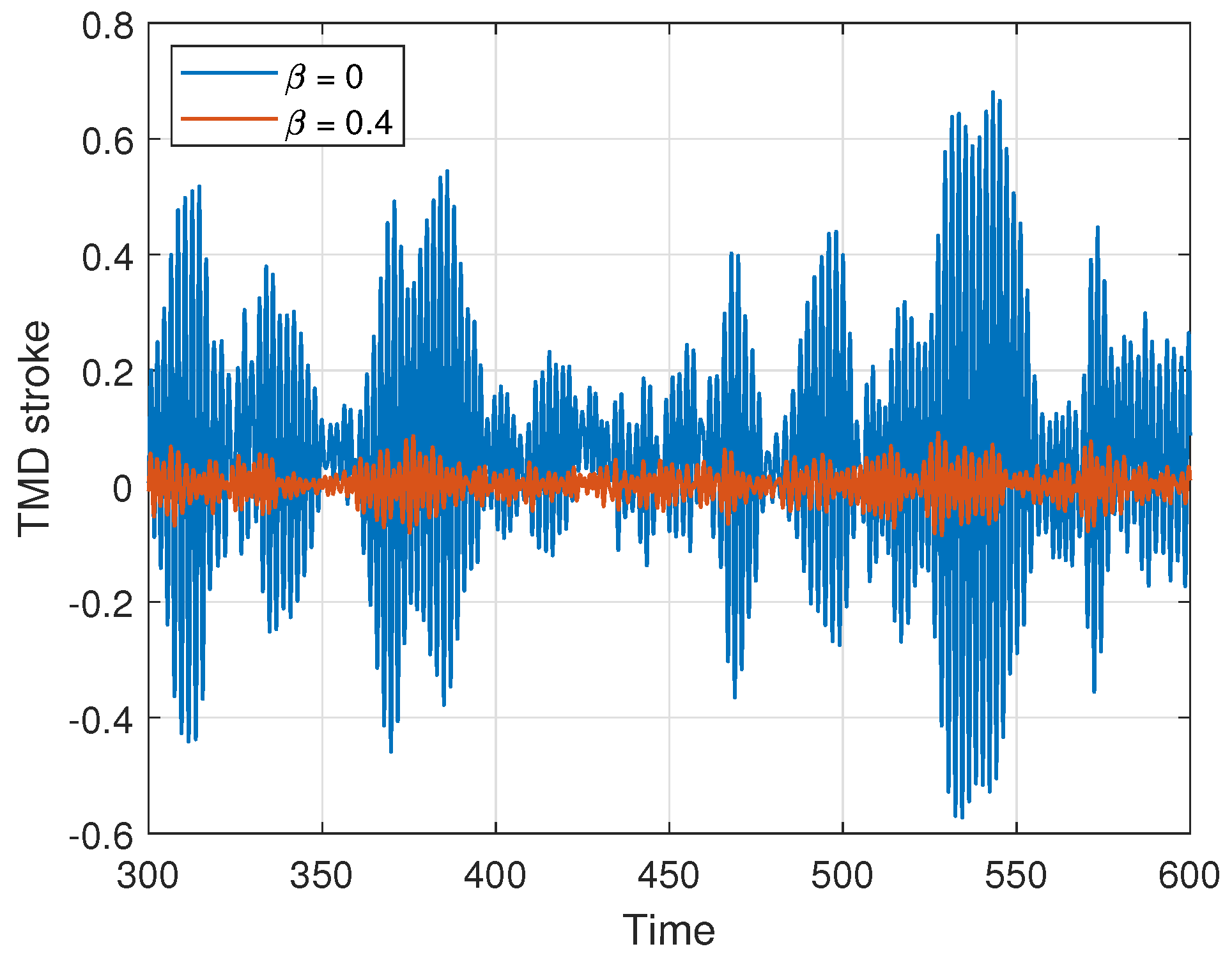
Another critical aspect of the TMDI is the drastic reduction of tuned mass stroke. The comparison of the damper stroke between a classical TMD and a TMDI is shown in Figure 13 and Figure 14. The authors also showed in [31] that increasing the mass ratio of the damper to improve vibration reduction is not a good idea for floating offshore wind turbines. Increasing the mass lumped on top of the tower will destabilise the floating platform. For more details on vibration control of floating offshore wind turbine towers using TMDI(s), refer to [31].

4. Conclusions

This paper demonstrated the use of Kane’s method for deriving equations of motion for spar-type floating offshore wind turbines, the steps of which apply to any multi-body system. The flexible multi-body wind turbine was modelled as a system comprising flexible and rigid members. Each component was modelled in its local coordinate system and transformed back to the inertial frame of reference using suitable transformation relationships. The derived model was benchmarked against the industry standard FAST [25]. Kane’s method was further used for the installation of an external damper. The excellent performance of the recently conceptualised TMDI in vibration control of floating offshore wind turbine towers was also presented.

It has been shown in this paper that Kane’s method vastly reduces the labor needed to derive equations of motion of a complicated multi-degree of freedom system. The resulting equations of motion are obtained as ODEs (rearrangement of terms not required), and the required vector multiplications can be performed on a computer. Therefore, the equations of motion are formed directly on a computer without human intervention, which is particularly desirable when working with many variables. The paper also demonstrates Kane’s method’s ease in installing an external device on the wind turbine.

As described in this paper, a large number of vector multiplications are performed on a computer to evaluate kinematics and kinetics of the system. A limitation of this method is the increasing computational time with increasing complexity of the system. However, with the rapid increase in computational power, it is unlikely to hinder performance.

Lastly, it is essential to mention that Kane’s method presented in this paper is general and applicable to any offshore/onshore wind turbine. Therefore, the steps are general to any dynamic system. This project envisages the use of this powerful modeling technique in extending the capabilities of the current wind turbine models. Some examples are as follows, installation of auxiliary devices [31], modification of current structural arrangements and components [61,62]. Investigation of improved foundation techniques and modeling future wind turbines. [63] etc. The developed knowledge will be used for modeling and dynamic analysis of the future larges-scale wind turbines.

References

- Council, G. Global Wind Report 2006; Global Wind Energy Council: Brussels, Belgium, 2006. [Google Scholar]
- Council, G. Global Wind Report 2021; Global Wind Energy Council: Brussels, Belgium, 2021. [Google Scholar]
- Murtagh, P.; Basu, B.; Broderick, B. Along-wind response of a wind turbine tower with blade coupling subjected to rotationally sampled wind loading. Eng. Struct. 2005, 27, 1209–1219. [Google Scholar] [CrossRef]
- Lackner, M.A.; Rotea, M.A. Passive structural control of offshore wind turbines. Wind Energy 2011, 14, 373–388. [Google Scholar] [CrossRef]
- Basu, B.; Zhang, Z.; Nielsen, S.R. Damping of edgewise vibration in wind turbine blades by means of circular liquid dampers. Wind Energy 2016, 19, 213–226. [Google Scholar] [CrossRef]
- Fitzgerald, B.; Basu, B.; Nielsen, S.R. Active tuned mass dampers for control of in-plane vibrations of wind turbine blades. Struct. Control Health Monit. 2013, 20, 1377–1396. [Google Scholar] [CrossRef]
- Fitzgerald, B.; Basu, B. Cable connected active tuned mass dampers for control of in-plane vibrations of wind turbine blades. J. Sound Vib. 2014, 333, 5980–6004. [Google Scholar] [CrossRef]
- Zhang, Z.; Basu, B.; Nielsen, S.R. Tuned liquid column dampers for mitigation of edgewise vibrations in rotating wind turbine blades. Struct. Control Health Monit. 2015, 22, 500–517. [Google Scholar] [CrossRef]
- Fitzgerald, B.; Sarkar, S.; Staino, A. Improved reliability of wind turbine towers with active tuned mass dampers (ATMDs). J. Sound Vib. 2018, 419, 103–122. [Google Scholar] [CrossRef]
- Zhang, Z.L.; Chen, J.B.; Li, J. Theoretical study and experimental verification of vibration control of offshore wind turbines by a ball vibration absorber. Struct. Infrastruct. Eng. 2014, 10, 1087–1100. [Google Scholar] [CrossRef]
- Fitzgerald, B.; Basu, B. A monitoring system for wind turbines subjected to combined seismic and turbulent aerodynamic loads. Struct. Monit. Maint. 2017, 4, 175–194. [Google Scholar]
- Cong, C. Stochastic Vibrations Control of Wind Turbine Blades Based on Wireless Sensor. Wirel. Pers. Commun. 2018, 102, 3503–3515. [Google Scholar] [CrossRef]
- Fitzgerald, B.; Basu, B. Structural control of wind turbines with soil structure interaction included. Eng. Struct. 2016, 111, 131–151. [Google Scholar] [CrossRef]
- Harte, M.; Basu, B.; Nielsen, S.R. Dynamic analysis of wind turbines including soil-structure interaction. Eng. Struct. 2012, 45, 509–518. [Google Scholar] [CrossRef]
- Buckley, T.; Watson, P.; Cahill, P.; Jaksic, V.; Pakrashi, V. Mitigating the structural vibrations of wind turbines using tuned liquid column damper considering soil-structure interaction. Renew. Energy 2017, 120, 322–341. [Google Scholar] [CrossRef]
- Achmus, M.; Kuo, Y.S.; Abdel-Rahman, K. Behavior of monopile foundations under cyclic lateral load. Comput. Geotech. 2009, 36, 725–735. [Google Scholar] [CrossRef]
- Carswell, W.; Arwade, S.R.; DeGroot, D.J.; Lackner, M.A. Soil–structure reliability of offshore wind turbine monopile foundations. Wind Energy 2015, 18, 483–498. [Google Scholar] [CrossRef]
- Dinh, V.N.; Basu, B. Impact of spar-nacelle-blade coupling on the edgewise response of floating offshore wind turbines. Coupled Syst. Mech. 2013, 2, 231–253. [Google Scholar] [CrossRef] [Green Version]
- Lackner, M.A. Controlling platform motions and reducing blade loads for floating wind turbines. Wind Eng. 2009, 33, 541–553. [Google Scholar] [CrossRef]
- Lackner, M.A. An investigation of variable power collective pitch control for load mitigation of floating offshore wind turbines. Wind Energy 2013, 16, 519–528. [Google Scholar] [CrossRef]
- Karimirad, M.; Moan, T. Wave-and wind-induced dynamic response of a spar-type offshore wind turbine. J. Waterw. Port Coast. Ocean Eng. 2011, 138, 9–20. [Google Scholar] [CrossRef] [Green Version]
- Waris, M.B.; Ishihara, T. Dynamic response analysis of floating offshore wind turbine with different types of heave plates and mooring systems by using a fully nonlinear model. Coupled Syst. Mech. 2012, 1, 247–268. [Google Scholar] [CrossRef] [Green Version]
- Karimirad, M.; Moan, T. Stochastic dynamic response analysis of a tension leg spar-type offshore wind turbine. Wind Energy 2013, 16, 953–973. [Google Scholar] [CrossRef]
- Wang, K.; Moan, T.; Hansen, M.O. Stochastic dynamic response analysis of a floating vertical-axis wind turbine with a semi-submersible floater. Wind Energy 2016, 19, 1853–1870. [Google Scholar] [CrossRef]
- Jonkman, J.M.; Buhl, M.L., Jr. Fast User’s Guide—Updated August 2005; Technical Report; National Renewable Energy Laboratory (NREL): Golden, CO, USA, 2005.
- Jonkman, J.M. Dynamics Modeling and Loads Analysis of an Offshore Floating Wind Turbine; University of Colorado Boulder: Boulder, CO, USA, 2007. [Google Scholar]
- Kane, T.R.; Levinson, D.A. Dynamics, Theory and Applications; McGraw Hill: New York, NY, USA, 1985. [Google Scholar]
- Lee, D.; Hodges, D.H.; Patil, M.J. Multi-flexible-body Dynamic Analysis of Horizontal Axis Wind Turbines. Wind Energy 2002, 5, 281–300. [Google Scholar] [CrossRef]
- Lee, D.; Hodges, D. Multi-Flexible-Body Analysis for Applications to Wind Turbine Control Design; School of Aerospace Engineering, Georgia Institute of Technology: Atlanta, GA, USA, 2003. [Google Scholar]
- Sarkar, S.; Chen, L.; Fitzgerald, B.; Basu, B. Multi-resolution wavelet pitch controller for spar-type floating offshore wind turbines including wave-current interactions. J. Sound Vib. 2020, 470, 115170. [Google Scholar] [CrossRef]
- Sarkar, S.; Fitzgerald, B. Vibration control of spar-type floating offshore wind turbine towers using a tuned mass-damper-inerter. Struct. Control Health Monit. 2020, 27, e2471. [Google Scholar] [CrossRef]
- Sarkar, S.; Fitzgerald, B.; Basu, B. Individual blade pitch control of floating offshore wind turbines for load mitigation and power regulation. IEEE Trans. Control Syst. Technol. 2020, 29, 305–315. [Google Scholar] [CrossRef]
- Sarkar, S.; Fitzgerald, B.; Basu, B. Nonlinear model predictive control to reduce pitch actuation of floating offshore wind turbines. IFAC-PapersOnLine 2020, 53, 12783–12788. [Google Scholar] [CrossRef]
- Larsen, T.J.; Hansen, A.M. How 2 HAWC2, The User’S Manual; Risø National Laboratory: Roskilde, Denmark, 2007.
- Stewart, G.; Muskulus, M. A review and comparison of floating offshore wind turbine model experiments. Energy Procedia 2016, 94, 227–231. [Google Scholar] [CrossRef] [Green Version]
- Staino, A.; Basu, B.; Nielsen, S.R. Actuator control of edgewise vibrations in wind turbine blades. J. Sound Vib. 2012, 331, 1233–1256. [Google Scholar] [CrossRef]
- Huang, N.E.; Chen, D.T.; Tung, C.C.; Smith, J.R. Interactions between steady won-uniform currents and gravity waves with applications for current measurements. J. Phys. Oceanogr. 1972, 2, 420–431. [Google Scholar] [CrossRef] [Green Version]
- Tung, C.C.; Huang, N.E. Influence of current on statistical properties of waves. J. Waterw. Harb. Coast. Eng. Div. 1974, 100, 267–278. [Google Scholar] [CrossRef]
- Thomas, G. Wave-current interactions: An experimental and numerical study. Part 1. Linear waves. J. Fluid Mech. 1981, 110, 457–474. [Google Scholar] [CrossRef]
- Silva, M.; Vitola, M.; Esperança, P.; Sphaier, S.; Levi, C. Numerical simulations of wave–current flow in an ocean basin. Appl. Ocean Res. 2016, 61, 32–41. [Google Scholar] [CrossRef]
- Ismail, N.M. Wave-current models for design of marine structures. J. Waterw. Port Coast. Ocean Eng. 1984, 110, 432–447. [Google Scholar] [CrossRef]
- Hedges, T. Some effects of currents on wave spectra. In Proceedings of the First Indian Conference in Ocean Engineering, Madras, India, 18–20 February 1981; Volume 1, pp. 30–35. [Google Scholar]
- Hedges, T.S.; Anastasiou, K.; Gabriel, D. Interaction of random waves and currents. J. Waterw. Port Coast. Ocean Eng. 1985, 111, 275–288. [Google Scholar] [CrossRef]
- Phillips, O.M. The Dynamics of the Upper Ocean; CUP Archive: Cambridge, UK, 1966. [Google Scholar]
- Azcona, J.; Palacio, D.; Munduate, X.; González, L.; Nygaard, T.A. Impact of mooring lines dynamics on the fatigue and ultimate loads of three offshore floating wind turbines computed with IEC 61400-3 guideline. Wind Energy 2017, 20, 797–813. [Google Scholar] [CrossRef] [Green Version]
- Jonkman, B.J. TurbSim User’S Guide: Version 1.50; Technical Report; National Renewable Energy Lab (NREL): Golden, CO, USA, 2009.
- Burton, T.; Jenkins, N.; Sharpe, D.; Bossanyi, E. Wind Energy Handbook; John Wiley & Sons: Hoboken, NJ, USA, 2011. [Google Scholar]
- Moriarty, P.J.; Hansen, A.C. AeroDyn Theory Manual; Technical Report; National Renewable Energy Lab.: Golden, CO, USA, 2005.
- Hansen, M.O. Aerodynamics of Wind Turbines; Routledge: Oxfordshire, UK, 2015. [Google Scholar]
- Ning, S.A. A simple solution method for the blade element momentum equations with guaranteed convergence. Wind Energy 2014, 17, 1327–1345. [Google Scholar]
- Ning, A.; Hayman, G.; Damiani, R.; Jonkman, J.M. Development and Validation of a New Blade Element Momentum Skewed-Wake Model within AeroDyn. In Proceedings of the 33rd Wind Energy Symposium, Kissimmee, FL, USA, 5–9 January 2015; p. 0215. [Google Scholar]
- Chen, L.; Basu, B.; Nielsen, S.R. A coupled finite difference mooring dynamics model for floating offshore wind turbine analysis. Ocean Eng. 2018, 162, 304–315. [Google Scholar] [CrossRef]
- Tjavaras, A.A. The Dynamics of Highly Extensible Cables. Ph.D. Thesis, Massachusetts Institute of Technology, Cambridge, MA, USA, 1996. [Google Scholar]
- Tjavaras, A.; Zhu, Q.; Liu, Y.; Triantafyllou, M.; Yue, D. The mechanics of highly-extensible cables. J. Sound Vib. 1998, 213, 709–737. [Google Scholar] [CrossRef]
- Gobat, J.; Grosenbaugh, M. Time-domain numerical simulation of ocean cable structures. Ocean Eng. 2006, 33, 1373–1400. [Google Scholar] [CrossRef]
- Fitzgerald, B.; Basu, B. Vibration control of wind turbines: Recent advances and emerging trends. Int. J. Sustain. Mater. Struct. Syst. 2020, 4, 347–372. [Google Scholar] [CrossRef]
- Zhang, Z.; Fitzgerald, B. Tuned mass-damper-inerter (TMDI) for suppressing edgewise vibrations of wind turbine blades. Eng. Struct. 2020, 221, 110928. [Google Scholar] [CrossRef]
- Marian, L.; Giaralis, A. Optimal design of a novel tuned mass-damper–inerter (TMDI) passive vibration control configuration for stochastically support-excited structural systems. Probabilistic Eng. Mech. 2014, 38, 156–164. [Google Scholar] [CrossRef]
- Giaralis, A.; Petrini, F. Wind-induced vibration mitigation in tall buildings using the tuned mass-damper-inerter. J. Struct. Eng. 2017, 143, 04017127. [Google Scholar] [CrossRef]
- Jonkman, J.M.; Butterfield, S.; Musial, W.; Scott, G. Definition of a 5-MW Reference Wind Turbine for Offshore System Development; National Renewable Energy Laboratory: Golden, CO, USA, 2009.
- Das, S.; Mohamed Sajeer, M.; Chakraborty, A.; Sarkar, S. Shape memory alloy-based centrifugal stiffening for response reduction of horizontal axis wind turbine blade. Struct. Control Health Monit. 2021, 28, e2669. [Google Scholar] [CrossRef]
- Mitra, A.; Sarkar, S.; Chakraborty, A.; Das, S. Sway vibration control of floating horizontal axis wind turbine by modified spar-torus combination. Ocean Eng. 2021, 219, 108232. [Google Scholar] [CrossRef]
- Fitzgerald, B.; Igoe, D.; Sarkar, S. A Comparison of Soil Structure Interaction Models for Dynamic Analysis of Offshore Wind Turbines. J. Phys. Conf. Ser. 2020, 1618, 052043. [Google Scholar] [CrossRef]
- Kane, T.; Ryan, R.; Banerjee, A. Dynamics of a cantilever beam attached to a moving base. J. Guid. Control Dyn. 1987, 10, 139–151. [Google Scholar] [CrossRef]
- Jonkman, J.M. Modeling of the UAE Wind Turbine for Refinement of FAST_AD; Technical Report; Citeseer: University Park, PA, USA, 2003. [Google Scholar]
Figure 1.
Schematic diagram of the degrees of freedom.
Figure 2.
Coordinate systems for Spar Type FOWT [30].
Figure 3.
Coordinate system for wave–current interaction definition.
Figure 4.
Pierson–Moskowitz spectrum with and without an underlying current.
Figure 5.
Submerged cable subjected to wave and current [30].
Figure 6.
TMDI installed inside tower [31].
Figure 7.
Schematic diagram of a tower with a TMDI placed on the top.
Figure 8.
Model verification: motion of the floating offshore wind turbine. (a) Blade 1 out-of-plane displacement; (b) Blade 1 in-plane displacement; (c) Tower top fore-aft displacement; (d) Tower to side-to-side displacement; (e) Nacelle yaw rotation; (f) Low speed shaft speed.
Figure 9.
Tower side-to-side displacement.
Figure 10.
Tower side-to-side displacement spectrum.
Figure 11.
Tower fore-aft displacement.
Figure 12.
Tower fore-aft displacement spectrum.
Figure 13.
Tower side-to-side damper stroke.
Figure 14.
Tower fore-aft damper stroke.