Commercial Energy Demand Forecasting in Bangladesh


1
Department of Agricultural Economics, Bangabandhu Sheikh Mujibur Rahman Agricultural University (BSMRAU), Salna, Gazipur 1706, Bangladesh
2
Faculty of Economics, Shandong University of Finance and Economics, Jinan 250001, China
3
Plymouth Business School, University of Plymouth, Drake Circus, Plymouth PL4 8AA, UK
*
Author to whom correspondence should be addressed.
Energies 2021, 14(19), 6394; https://doi.org/10.3390/en14196394
Submission received: 26 August 2021
/
Revised: 27 September 2021
/
Accepted: 2 October 2021
/
Published: 6 October 2021
Abstract
:Although both aggregate and per capita energy consumption in Bangladesh is increasing rapidly, its per capita consumption is still one of the lowest in the world. Bangladesh gradually shifted from petroleum-based energy to domestically sourced natural-gas-based energy sources, which are predicted to run out within next two decades. The present study first identified the determinants of aggregate commercial energy and its three major components of oil, natural gas, and coal demand for Bangladesh using a simultaneous equations framework on an annual database covering a period of 47 years (1972–2018). Next, the study forecast future demand for aggregate commercial energy and its three major components for the period of 2019–2038 under the business-as-usual and ongoing COVID-19 pandemic scenarios with some assumptions. As part of a sensitivity analysis, based on past trends, we also hypothesized four alternative GDP and population growth scenarios and forecast corresponding changes in total energy demand forecast. The results revealed that while GDP and lagged energy demand are the major drivers of energy demand in the country, we did not see strong effects of own- and cross-price elasticities of energy sources, which we attributed to three reasons: subsidized low energy prices, time and cost required to switch between different energy-mix technologies, and suppressed energy demand. The aggregate energy demand is expected to increase by 400% by the end of the forecasting period in 2038 from its existing level in 2018 under the business-as-usual scenario, whereas the effect of COVID-19 could suppress it down to 300%. Under the business-as-usual scenario, the highest increase will occur for coal (3.94-fold), followed by gas (2.64-fold) and oil (2.37-fold). The COVID-19 pandemic will suppress the future demand of all energy sources at variable rates. The ex ante forecasting errors were small, varying within the range of 3.6–3.7% of forecast values. Sensitivity analysis of changes in GDP and population growth rates showed that forecast total energy demand will increase gradually from 3.58% in 2019 to 8.79% by 2038 from original forecast values. Policy recommendations include capacity building of commercial energy sources while ensuring the safety and sustainability of newly proposed coal and nuclear power installations, removing inefficiency of production and distribution of energy and its services, shifting towards renewable and green energy sources (e.g., solar power), and redesigning subsidy policies with market-based approaches.
1. Introduction
Energy is one of the crucial prerequisites of any economic activity. Increased energy consumption is a proxy for increased economic activities unless inefficiency arises. In the last five and half decades, global energy consumption has doubled and the estimated figure in 2019 was 100.17 quadrillion Btu [1,2]. However, the projection of energy demand doubling from its level in 2005 is only 25 years, i.e., 2030 [3], implying that energy demand will accelerate at a much higher rate in the future. The increasing demand imposes additional challenges of environmental consequences and ensuring equitable access of the poor, particularly in regions or countries with limited endowments. In response, countries require capacity building and planning for both supply- and demand-side strategies. While capacity building, particularly focusing on renewable sources, is the core strategy for many countries, many are trying to boost such strategies through redesigning subsidy policies [4]. For instance, by 2050, China plans to generate 85% of its total energy from nonfossil fuel, through technological innovation and enhancing efficiency [5]. Similarly, redesigning subsidy policies aiming to control wasteful use by increasing efficiency is another option [4].
In the race against increasing energy use occurring around the world, Bangladesh is no exception; total energy consumption has increased 11.5-fold compared to its level in the early 1980s from 0.12 quad Btu in 1980 to 1.418 quad Btu in 2017 [6]. Consumption of energy is expected to increase even more rapidly in the near future since the level of urbanization and industrialization is gradually increasing. For instance, the value of the industrialization intensity index of Bangladesh is higher than any time in the history and its growth rate outpaces world’s median level [7]. It is widely recognized that the energy sector is critical in accelerating GDP growth, although the causality of relationship between the two can run both ways [8]. Ensuring uninterrupted energy supply is particularly critical for a country like Bangladesh where the conventional three fossil fuel sources (e.g., oil, natural gas, and coal) supply more than 99% of the total commercial energy consumption, of which natural gas is the only indigenous energy source [6]. Fuel import constitutes around 11% of total merchandise imports [9]. The high dependency on international energy markets makes the country’s development extremely vulnerable to external shocks. It is noteworthy to mention that energy prices are more volatile than those of most other products [10] and a 10% rise in oil price will result in a 0.5% loss of GDP [11]. Under such circumstances, it is important to estimate and understand future energy demand so that the country can appropriately plan for capacity increase and investments in this sector. On the demand side, it requires adopting policies to develop technologies, increase energy use efficiency, and promote green production and ecofriendly lifestyles. On the supply side, along with capacity building, different fiscal instruments (e.g., environmental tax, carbon tax, and trading) and tax policies can be designed to facilitate the shift from fossil- to nonfossil-based power generation [5]. Such planning is particularly important for the poorer segment of the population who lack adequate and affordable access to energy, a key to inclusive growth [4].
Therefore, taking stock of the existing energy use scenario and forecasting future demand based on the examination of existing and past trends is crucial in order to identify the trajectory of energy demand for the future. The importance has been highlighted by the recent COVID-19 global pandemic, which has exerted an unprecedented braking effect on the economies of all major developed and developing countries for an indefinite period. The global-level impact will be reduced trade, since countries will be experiencing both demand- and supply-side shocks, though the level will vary across countries and regions [12,13]. This has led to adjustments in predictions of economic growth due to COVID-19 by various international organizations including the World Bank and International Monetary Fund (IMF), in addition to national governments.
Given this backdrop, the specific objectives of this study were to (a) estimate and identify the determinants of aggregate commercial energy demand and its three major sources, oil, natural gas, and coal, using the longest possible annual data for Bangladesh covering the period 1972–2018; (b) forecast aggregate commercial energy demand and its three major sources, oil, natural gas, and coal, for the next 20 years (2019–2038) under two scenarios: (i) business as usual, and (ii) taking into account the predicted depressing effect of COVID-19 on the economy.
The paper is organized as follows. Section 2 provides an overview of the energy scenarios of selected Asian countries as well as Bangladesh to set the context, provides a brief review of energy demand models commonly used in the literature including energy demand models used for Bangladesh in particular, including their limitations, and outlines our contribution to the existing literature. Section 3 presents the methodology and describes the data. Section 4 presents results. Section 5 synthesizes and discusses the results. Finally, Section 6 concludes and draws policy implications.
2. Energy Use Scenarios and Energy Demand Models
2.1. Recent Energy Scenarios in Selected Asian Countries
If Asia can sustain a 6% annual growth rate of GDP until 2035, then the continent will contribute 44% to the global GDP and consume 51% to 56% of the global energy, almost doubling its consumption level from 28% in 2010. Meeting this growing energy demand is a serious challenge for Asia, as the majority of the countries in the continent depend on international markets for petroleum and natural gas, while coal is produced largely domestically. Furthermore, the continent’s plan for renewable energy and nuclear power is not adequate to meet the growing demand [4].
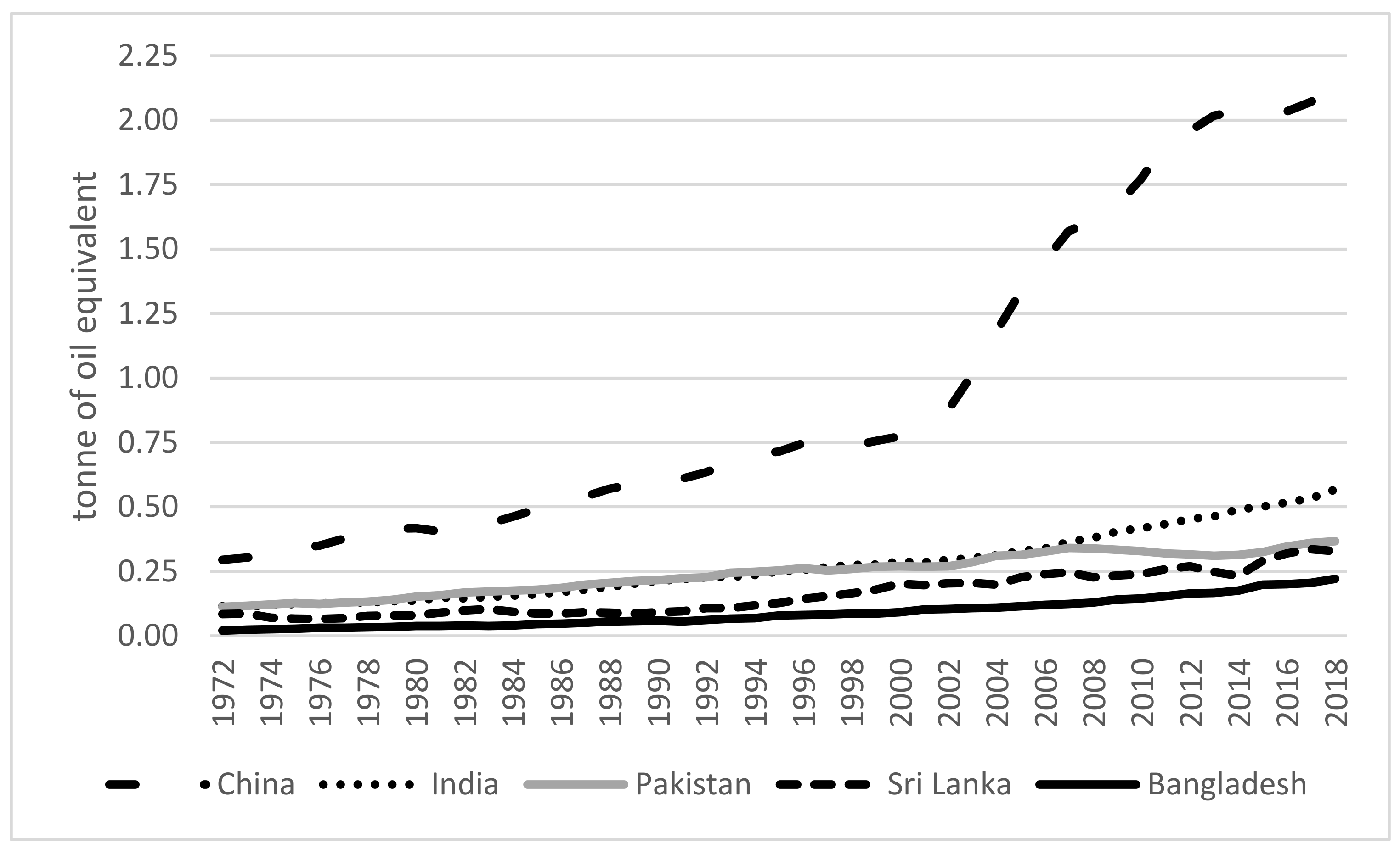
Figure 1 presents the per capita energy consumption of some selected Asian countries, including Bangladesh, and the associated growth rates in consumption are presented in Table 1 and Table 2. We compared Bangladesh with her neighboring countries India and Pakistan, since the three countries share similar economic structures and inherited same imperial legacy. China was taken as the ideal yardstick, being one of the largest economies with impressive growth. Not surprisingly, China had the highest per capita consumption, while Bangladesh had the lowest among the countries under consideration. Energy consumption in China has grown at a much faster rate than in other countries, particularly in the 21st century, widening the gap with other countries. In 1972, per capita energy consumption in China was 2.58, 2.62, 3.47, and 14.66 times higher than in India, Pakistan, Sri Lanka, and Bangladesh, respectively. In 2018, per capita consumption in China further increased by a further 1.46, 2.22, and 1.87 points above India, Pakistan and Sri Lanka, respectively. Bangladesh is the only exception with a reduced gap, though China still has around 10-fold higher per capita consumption. In terms of per capita consumption growth, Bangladesh had the highest growth rate, followed by China, Sri Lanka, India, and finally Pakistan. China and India had relatively higher growth rates in the 21st century, whereas the other three countries had higher rates during the past century.
In the last four and half decades, per capita energy consumption in Bangladesh has increased annually at a rate of 4.81%, the highest among the countries under consideration (Table 1). Pakistan had a relatively higher per capita consumption rate than India until 1977. In recent times, Sri Lanka has begun to minimize the gap in consumption with Pakistan. Sri Lanka had has a very low (1.22%) growth rate in consumption in the 21st century. Perhaps this stagnancy in consumption, at least compared to other countries, reflects the sociopolitical and economic turbulence experienced in Sri Lanka in recent years. Pakistan is a country experiencing severe energy issues for several reasons, including political and economic turbulence, costly fuel sources, chronic electricity and natural gas scarcities, circular debt, inadequate transmission and distribution systems, etc. [4,14]. The country is a net importer of crude oil and refined products, wherein crude oil imports in 2015 grew by around 12% over the year [14]. The Asian Development Bank has estimated that the chronic power crisis in Pakistan reduced the GDP growth rate by 2–3% in 2013. The power crisis has also largely contributed to the slowdown of large-scale manufacturing industries, which grew at only 1.2% and 2.8% in 2012 and 2013, respectively [4].
2.2. Energy Scenario in Bangladesh
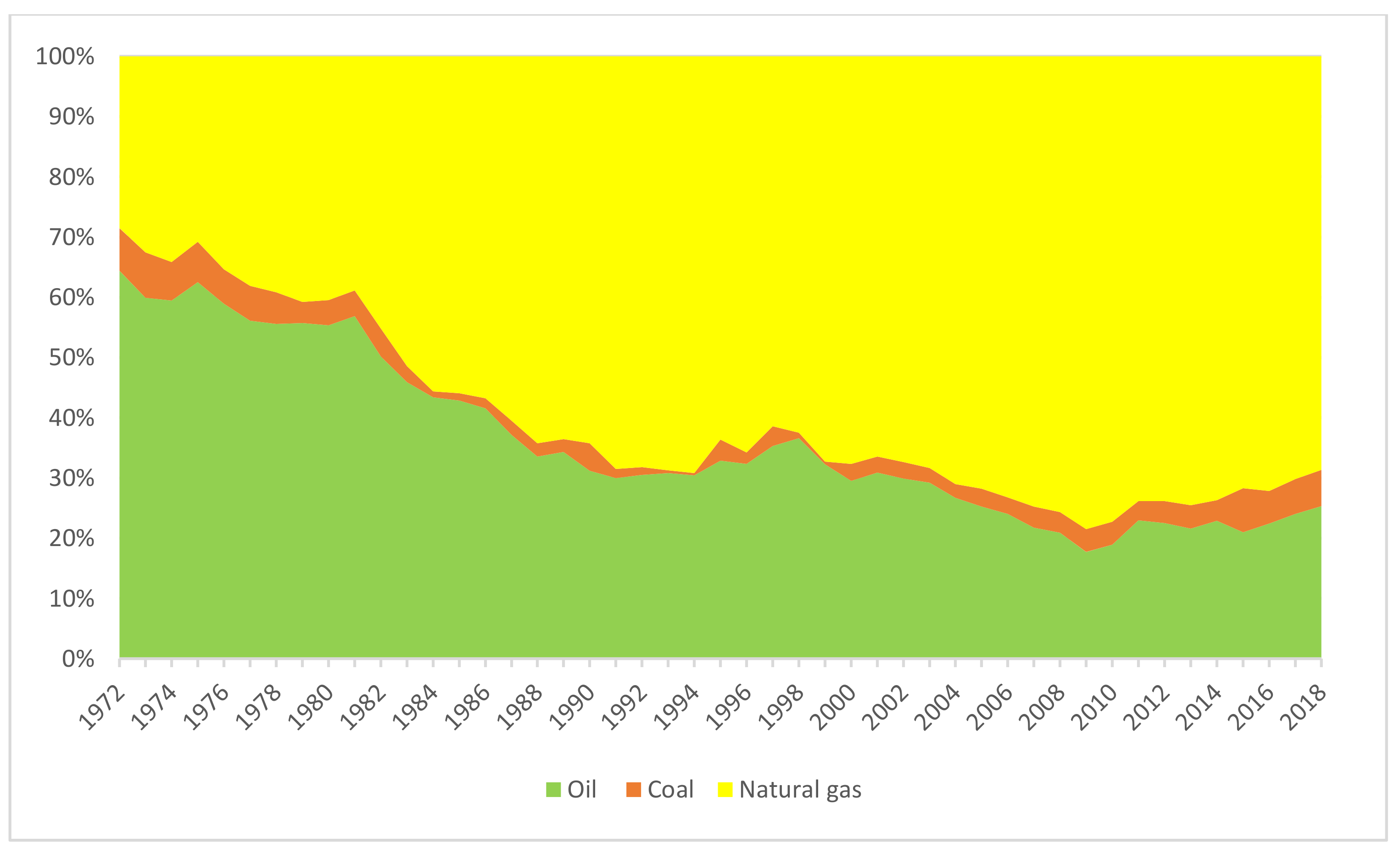
Figure 2 presents the total energy consumption in Bangladesh during the period of 1972–2018, whereas the share of consumption by source is presented in Figure 3. Total energy consumption in Bangladesh in 2018 was 1491.62 petajoules, which was only 0.28% of the world consumption [15]. Since independence on 16 December 1971, the total energy consumption in Bangladesh has increased at a rate of 6.48% p.a. and the estimated figure in 2018 was 27 times higher than that of 1972 (Figure 2 and Table 2). In terms of per capita energy consumption, Bangladesh is positioned 158th in the world [6]. In terms of production of energy, the country ranked 49th in the world in 2017, which is commendable progress compared to her position as 79th in 1980 [6], largely due to increased extraction of natural gas (Figure 2).
Traditionally, imported petroleum was the major source of commercial energy in Bangladesh. After the discovery of several major gas fields, and given that natural gas is cheaper than petroleum and less vulnerable to external price shocks, the government adopted policies for promoting use of natural gas since 1970s. Some such policies include gas exploration through international and state-owned companies, gas pipeline connections to industries and households, encouraging compressed natural gas (CNG) as a transportation fuel, etc. Consequently, after the beginning of the 1980s, natural gas took the leading position and its consumption during the 1972–2000 period grew at a rate of 10.64% p.a., which was more than double the rate of petroleum growth at 4.49% p.a. Although the growth rate of natural gas later reduced to 6.23% p.a., it is still higher than the growth rate of petroleum at 4.58% p.a. However, since the natural gas stocks may run within a decade, there has been some shift in government policies in terms of restricting new connections and increasing gas prices. Following this, the share of natural gas in total commercial energy consumption has been decreasing in the past decade. In 2018, natural gas constituted almost 69% of the total commercial energy consumption, with around 80% in 2009. The share of petroleum is constantly decreasing and in 2018 it contributed around a quarter of the total. Interestingly, the contribution of coal to total energy consumption gradually decreased from 7% in the early 1970s to almost nil. However, after 2000, coal consumption grew at a rate of 11.35% p.a. against a 0.44% growth rate in 1972–2000, making it a relatively important source in recent years. In absolute terms, compared to the 1972 level, coal consumption increased 23-fold. This growth in coal consumption is due to the government policy of increasing electricity generation mainly through coal-based power stations. This policy shift is largely driven by several factors. In the international market, the supply of coal is more stable and diversified as it is more widely available across the world and its price is more stable than those of oil and natural gas [16]. Understanding this, the government has planned to rely more on coal. For instance, the government has planned to install 7500 MW of coal-based power plants by 2021 [16], whereas the total electricity generation capacity in 2017–2018 was 15,953 MW [17], indicating that almost 50% of total power generation capacity is to come from coal-based production sources.
2.3. Energy Demand Models
Due to its immense importance and cross-cutting nature, energy demand has been extensively studied in the literature. The available literature is diverse in nature, focus, and methodology used. Suganthi and Samuel [18] did an extensive review and listed 12 different types of forecasting techniques applied in the literature. Accuracy of forecast can be improved by adopting sophisticated techniques such as genetic algorithms, fuzzy logic, SVR, PSO, neural network, AGO, etc. [18,19]. For instance, Kandananond [20] compared results from autoregressive integrated moving average (ARIMA) and artificial neural network (ANN) models to the historical data regarding electricity demand in Thailand from 1986 to 2010 and found that ANN produces better forecasts. Ghalehkhondabi et al. [19] categorized available technologies under two broad categories: casual methods (e.g., regression models, econometric models, cointegration models, neural networks, etc.) and historical-data-based methods (e.g., annual series, Grey prediction, autoregressive models, etc.). While forecasting future demand or consumption based on historical data is perhaps the more commonly used approach, many have tried to forecast by exploring the casual relationships between energy demand and the related explanatory factors representing economic (e.g., GDP/GNP, price), technology (e.g., technology development and energy efficiency, etc.), climatic factors, and the demography of a nation or economy [19].
All these techniques have their own pros and cons [18,19]. For instance, forecasting using historical data (e.g., annual series, grey prediction, and autoregressive models) is relatively simpler [19], typically requiring longer time-series data [21] but unable to capture dynamism in energy demand [22]. Although dynamism, whether linear or nonlinear, can be captured through regression analysis, the analysis is challenging since it requires complicated input factors and longer annual data to make sensible predictions [19,21].
2.4. Energy Demand Models in Bangladesh
Exploring the literature specific to Bangladesh, we observed certain common patterns resulting in specific limitations. First, Wadud et al. [22] reported that forecasting based on historical data is the common practice in Bangladesh. Such data exploration techniques predict future values based on past values and hence cannot capture the effects of recent socioeconomic and policy dynamism. Second, the available literature that investigated dynamism in energy demand did not focus on aggregate demand. For instance, Wadud et al. [22] and Das et al. [23] focused on natural gas only, while Mondal et al. [24] applied an accounting-type planning model for the power sector alone. In the most recent study, Debnath and Mourshed [25] explored energy demand for Bangladeshi rural households only. Even Kabir and Sumi [26] applied the sophisticated method of an integrated fuzzy Delphi method with ANN to predict the demand of a power engineering company only. For policy purposes, aggregate demand forecasting is the most appropriate and relevant approach. Most importantly, these sector-specific demand exercises ignored full dynamism in the derived demand. For instance, while some focused only exploring the relationship between demand and GDP/income (e.g., [23,27]), others did not go beyond own-price elasticity—a trend common in both Bangladesh-specific (e.g., [22]) and cross-country analysis [28]. Though Paul and Uddin [29] explored the causality between aggregate energy demand and output through a variable autoregressive model, they did not consider the effect of price. Third, in Bangladesh we found forecasting of aggregate energy demand by Rahman [30], which is outdated. Rahman [30] used data from 1972/73 to 1990/91 to predict energy demand up to 2019/20. Therefore, his prediction did not incorporate the extraordinary changes that the energy sector in Bangladesh has gone through since 2000. As a result, his predicted estimates are much lower than the actual consumption levels beyond 2000. For instance, Rahman’s [30] estimated demand for 2015 is around 30% lower than the actual consumption. The recent COVID-19 pandemic situation further raises concern about the old estimates. Fourth, much of the available research suffers from statistical flaws. For instance, Wadud et al. [22] employed a log-linear Cobb-Douglas model with annual data, but they did not perform the required statistical tests to ensure that their data fulfilled all the classical assumptions required in an OLS model. Fifth, since time length covered is critical in forecast accuracy [19,21], one may have doubts about the forecasts available for Bangladesh. Utilizing data for only a decade, Mondal et al. [24] forecast for the next 20 years, whereas Paul and Uddin [29] considered the highest possible 40 years.
Against this backdrop, we utilized the temporal advantage that we had compared to our precedents and used longer time-series than used by any available Bangladesh-specific literature to explore determinants of aggregate energy demand and its three common sources (i.e., coal, fuel, and natural gas). Our contribution to the existing pool of literature is three-fold. First, we modeled aggregate and source-wise energy demand in Bangladesh by considering energy demand as a derived demand in a production process. We derived complete dynamism in energy demand by considering GDP and own and cross price of the energy sources. Furthermore, we included dynamism in the model by considering lagged energy demand of the preceding two years as regressor. Second, since we performed all the statistical tests required for time-series data, we claim that our models are more accurate. Third, instead of the common practice of predicting future values based on past data, we forecast based on model estimates. We also explored a longer time-series than has been utilized so far in Bangladesh-specific literature. Hence, we believe that our forecasts are more accurate than previous estimates, since our estimations accounted for dynamism in energy demand. Finally, we also tried to capture the possible effect of the currently ongoing COVID-19 pandemic on future demand. To our knowledge, this is the first effort to incorporate the effect of COVID-19 pandemic in forecasting future energy demand for Bangladesh and elsewhere using a proper modeling framework. Since we adopted a well-established approach by ensuring that all the statistical prerequisites hold, we claim that our research provides insights that are also relevant for other developing countries that share similar energy demand scenarios.
3. Methodology
3.1. Data
This study is based on secondary data collected from multiple sources. The commercial energy consumption data by source for 47 years (1972–2018) were collected from OurWorldInData.org, where they were actually extracted from the BP Statistical Review (http://www.bp.com/statisticalreview, accessed on 3 March 2020). The real GDP (at 2010 constant price) and population data were taken from the World Bank Development Indicators. The real prices of Australian coal, natural gas from the USA, and the world average crude oil were collected from the World Bank Commodity Price Data (the Pink Sheet). The energy consumption data were then converted to petajoules, whereas the price data were converted into real USD/petajoule. The energy consumption, GDP, and population are total annual estimates, whereas prices are annual averages.
3.2. Modeling Energy Demand
In a production process, energy demand is a derived demand. The demand is derived from the demand of buyers of the output. In general, the demand for an input or a factor of production depends on its own price, the prices of other inputs that can substitute for or complement that input, the parameters of the production function that describes the technical transformation of that input into an output, and the price of output(s) being produced. Energy demand may depend on many other external factors, including consumers’ income, changes in policy and technology, environmental factors, structural changes, etc. Information on many of these drivers is difficult to extract, particularly in developing countries; thus, GDP/income and price are the two most commonly used explanatory variables for explaining changes in energy demand (e.g., [31,32]). This is also true for Bangladesh where even the effect of substitute/complementary prices are ignored. Wadud et al. [22], for instance, considered only natural gas prices while explaining natural gas demand. Tzeng developed several translog models where real energy price index, GDP, and one-year lag were considered while estimating total energy demand [32].
We used GDP, population, energy prices, and lagged values of energy consumption to model energy demand in Bangladesh. We developed two variants of the aggregate energy demand function, one with the weighted average price of coal, gas, and oil and another with individual prices of the three fuel types. We also modeled individual demands for coal, natural gas, and oil. Instead of per capita demand, we used aggregate demand as policy makers are more interested in total demand. In case of GDP, we used per capita instead of total GDP to avoid possible multicollinearity between total GDP and population. Depending on the formation of the individual models, we used weighted average energy price or individual energy prices.
3.2.1. OLS Model for Aggregate Energy Demand
Among the different competing functional forms (e.g., linear, log-linear, semilog, translog, etc.) we chose the commonly used log-linear Cobb-Douglas functional form to model aggregate energy demand in Bangladesh. The model, estimated using ordinary least squares (OLS) estimation techniques, satisfied the classical Gauss-Markov assumptions, and provided estimators that possess the best linear unbiased estimator (BLUE) properties. Another unique feature of the model is that the parameter estimates can be directly read as production elasticities. Furthermore, such a log-linear type of model can better represent nonlinearity of the production structure [33]. According to the Cobb-Douglas model, the aggregate energy demand can be modeled as follows:
The logarithmic form of the above equation with error term is as follows:
where is the aggregate energy demand in Bangladesh measured in petajoules; is GDP per capita (constant 2010 USD); is population of Bangladesh; is weighted average real price (USD/petajoule) of coal, gas, and oil; , , and are the parameters to be estimated; and is the error term. The subscript refers to year. Unlike other input demands, there is lag between energy demand and explanatory variables. For instance, energy demand does not respond immediately to GDP changes, rather requiring significant capital investment and technological interventions to bring in additional supply to meet the demand. The literature suggests using a limited number of lags (one or two), since increasing lags requires trade-offs to be made with degrees of freedom and multicollinearity [34,35]. Gujarati cautioned about data mining in the process of searching for appropriate lags [34,35]. Though several commonly used goodness-of-fit tests (e.g., AIC, BIC, FPE, and R2) can be used to select appropriate lag lengths, following Liew we conducted the AIC test, which performs better than others when the sample is small (n < 60) [36]. Since we found small AIC values when two-year lags were introduced instead of none or one-year lag, we included two-year lags of energy demand alongside other explanatory variables to capture the dynamic time-dependent nature of energy demand. The final model was thus
We termed the above model ‘model 1′. The other aggregate demand model was termed ‘model 2′, wherein all the specifications are same except instead of weighted price; we used coal, gas, and oil prices. The logarithmic form of the ‘model 2′ was as follows:
where , , and are the real prices (USD/petajoule) of coal, gas, and oil in year , respectively.
In the analysis using annual data, the independent variables were not random since the data across years were from the same unit. This raised concern about serial autocorrelation among errors of the successive years, which would be a violation of the classical Gauss-Markov assumptions. In the presence of serial autocorrelation, the OLS estimators no longer have minimum variance and remain efficient relative to other linear and unbiased estimators. Ultimately, the estimators are no longer BLUE and the associated t-test and goodness-of-fit (F test and ) results are not valid [34]. There are additional challenges in time-series analysis to ensure that the Gauss-Markov assumptions of endogeneity, homoscedasticity, and no autocorrelation are fulfilled. We did a series of required tests and found that all the required assumptions were fulfilled for our analysis (reported in bottom of Table 3 and discussed later) and we did not require an alternative estimation method such as generalized least square.
3.2.2. SURE Model for Coal, Natural Gas, and Oil Demand
Along with aggregate demand, it is important to know demand by energy sources. Similarly to the aggregate energy demand model in Equation (4), we tried separate models to explain coal, gas, and oil demand. Since these three are parts of the same economic settings and their demands are explained by the same set of explanatory variables, their individual demand equations may be interlinked. Under such possibilities, instead of estimating the three demand equations separately, they should be jointly estimated through Zellner’s suggested Seemingly Unrelated Regression Estimation (SURE) procedure, including testing whether the error terms of the individual equations are correlated [37,38,39]. In a SURE model, jointness of equations is explained by the structure of the model and the covariance matrix of associated disturbances. The unique feature of this model is the additional information generated through the identification of jointness across equations, which remains unidentified when equations are estimated separately [40].
The aggregate demand function expressed in Equation (4) comprises three separate equations for coal, gas, and oil demand in the following form:
where is the demand for th energy source in year which is to be explained in the th regression and is the th explanatory variable in year in the th regression equation. The list of explanatory variables is same as that used in Equation (4).
The aggregate energy demand is vector with elements ; is matrix, the columns of which represent the observations on an explanatory variable in the th equation; . is a . vector with elements
; and is a vector of disturbance. The three equations can be further expressed as follows:
which is from , and each of the equations are the classical regression model with conventional assumptions. We estimated the model using the sureg command in STATA 14 [41], which is by default estimated through OLS. The correlation between the errors of the equations can be estimated through the test suggested by Breusch and Pagan [42]. When there is number of equations and number of observations, the statistic is as follows:
where . is the estimated correlation between the residuals, which is distributed as . with degrees of freedom.
Acknowledging the possible interdependence among the three equations of the SURE model under consideration, we applied a symmetry restriction defining that coefficients of same fuel type across equations are same (i.e., ). In addition, we applied an additional homogeneity condition defining that summation of all the cross-price elasticities across models is zero (i.e., ).
3.3. Forecasting Future Energy Demand
We used the OLS and SURE model estimates to forecast energy demand in Bangladesh for two decades (2019–2038). The strategies we followed here can be classified into two broad categories. First, to forecast demand, we need to know the future values of the independent variables. We estimated the annual exponential growth rate of all the explanatory variables as the parameter in . This growth rate was then used to extrapolate the existing explanatory variables for next 20 years. Afterwards, using the estimated coefficients of the OLS and SURE models, we forecast the aggregate, coal, gas, and oil demands using the forecast and forecast-solve commands in STATA 14. In addition, we did an in-sample forecast using the forecast and forecast-solve commands and calculated the 95% upper and lower bounds of the confidence interval to check accuracy of our forecasts.
3.4. Sensitivity Analysis: Alternative Scenerios including COVID-19
Any such exercise will be irrelevant if the effect of the recent COVID-19 pandemic is overlooked. Extracting Kilian’s learning, which noted four different types of crude oil real price shocks including structural changes at both supply and demand sides [43], we can assume types of shock in energy demand as a consequence of COVID-19. For instance, due to lockdown-related limited economic activities, one may argue for price shock as energy demand will be reduced. At the supply side, lockdown may reduce energy supply and increase the associated cost, which will increase the price. Again, in extreme situations, one may argue for reduced demand and price, as the death toll is increasing. However, since the turbulence is not yet over, the real effect is still unknown and different organizations are predicting differently. In our case, we assumed the most unavoidable one, impact on GDP, for which some data were available for estimation. We did not assume population to decrease as the death rate may not be that high. We also assumed other prices to follow the normal trend as the real situation is yet to be understood.
The International Monetary Fund (IMF), for instance, predicted only a 2% growth rate for Bangladesh during 2019–2020, followed by a very high growth rate of 9.5% during 2020–2021 [44]. Meanwhile, the World Bank forecast a 5.2% reduction in global GDP in 2020 [45]. We took this World Bank forecast and assumed that GDP in Bangladesh for consecutive five years (2020–2024) will drop by 5% every year instead of recovering immediately after the COVID-19 pandemic is over, i.e., actual reduction of 2020 GDP by 5% of 2019 GDP and so forth.
GDP and population in the future have a certain degree of uncertainty which may affect future commercial energy demand. This requires sensitivity analysis through the construction of different scenarios. Exploring the World Bank’s historical data, we estimated the past GDP and population growth rates for Bangladesh and added these rates to the forecast values. We assumed the following four additional scenarios:
Scenario 1: 4.92% GDP growth rate (i.e., the GDP growth rate between 1972 and 2018) and 1.92% population growth rate (i.e., the population growth rate between 1972 and 2018);
Scenario 2: 4.92% GDP growth rate (i.e., the GDP growth rate between 1972 and 2018) and 1.34% population growth rate (i.e., the population growth rate between 2000 and 2018);
Scenario 3: 6.05% GDP growth rate (i.e., the GDP growth rate between 2000 and 2018) and 1.92% population growth rate (i.e., the population growth rate between 1972 and 2018)
Scenario 4: 6.05% GDP and 1.34% population growth rate (i.e., the population growth rate between 2000 and 2018)
4. Results
4.1. Hypothesis Testing and Model Validation
4.1.1. The OLS Models for Aggregate Demand
Our application of OLS estimation technique to time-series data required testing whether the classical Gauss-Markov assumptions, particularly those related to endogeneity, homoscedasticity, and no autocorrelation, held for our data. We did a series of related tests, which are presented in the middle section of Table 3. The first of these tests was the Jarque-Bera test for normality. The insignificant test statistics imply that the residual terms in both the models followed normal distribution. To test homogeneity, we performed the Breusch-Pagan test, where test results confirmed that in both models, the error variances were equal, i.e., there was homoscedasticity. To check stationarity, we performed a couple of tests. The first test was the Durbin-Watson test for the first-order serial correlation in the disturbance, assuming that all the regressors were strictly exogenous. Since, in both the models, the estimated Durbin-Watson test statistics were near 2, we can argue that there was less chance of autocorrelation. In addition, we performed the Breusch-Godfrey test for higher-order serial correlation in the error terms. Unlike the earlier test, this test does not require all the regressors be strictly exogenous. According to the test results for both the models, we failed to reject the null hypothesis of no serial correlation. The above test results confirmed that all the Gauss–Markov assumptions critical for time-series analysis were not violated, and hence the estimators of the chosen OLS models still hold BLUE properties.
4.1.2. The SURE Model for Gas, Coal, and Oil Demand
The Breusch-Pagan test statistics presented in the lower part of Table 3 shows that we can reject the null hypothesis that the correlation between error terms across equations is zero. This indicates that the coal, gas, and oil demand are actually interlinked and hence our choice of SURE model structure was appropriate and valid. The root mean square error (RMSE), which is the square root of the variance of the residuals, indicates absolute fit of the model to the data, i.e., how close the observed data points are to the model’s predicted values. Our estimated very low RMSE values for the oil and gas equations confirmed that the chosen model was well-fitted, but for the coal equation the model was a moderate fit. The highly significant F-statistics for all the three demand equations imply that the explanatory variables jointly explained the variations in demand for these individual energy types well.
4.2. The Model Results
Determinants of Energy Demand
The first two columns of Table 3 with figures present the results of the two OLS models for aggregate energy demand in Bangladesh, whereas the SURE model results for demand by three common energy sources are presented in the last three columns.
In both the OLS models for aggregate demand, the estimated parameters for all the explanatory variables were almost identical. We found that the aggregate and oil demands were income-inelastic, whereas coal demand was highly income-elastic. A 1% increase in per capita income increased aggregate energy demand by 0.31% and 0.33% in model 1 and model 2 respectively. Similarly, for a 1% increase in per capita income, oil demand increased by 0.36% and coal demand increased by a substantial 2.25%, which was in the elastic range. A 1% increase in population led to 1.53% to 1.59% growth in aggregate energy demand. The one-year lag energy variable had a positive significant effect across all models, thereby confirming dynamism in energy demand. Among the own- and cross-price variables used, except weighted energy price in model 1 and oil price in the equation for oil demand, none had any statistically significant effect. In line with the well-established negative association between price and demand, we found a 0.029% reduction in aggregate demand following a 1% increase in weighted average price of energy. Oil demand was also price-inelastic, where a similar magnitude of increase in oil price reduced oil consumption by 0.075%.
4.3. Forecasting Energy Demand
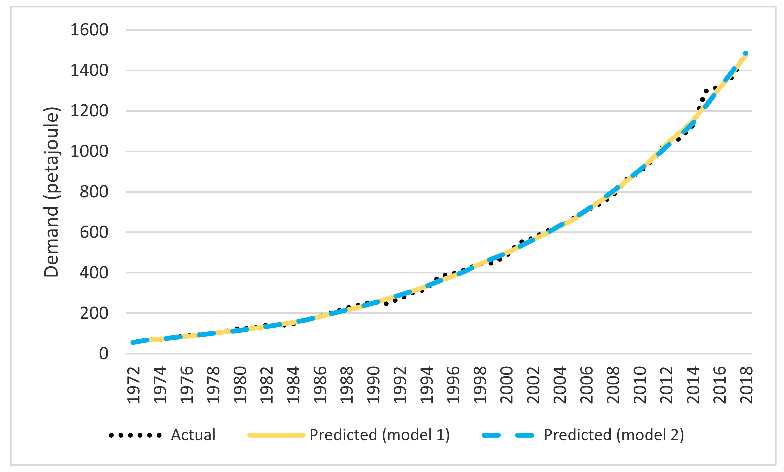
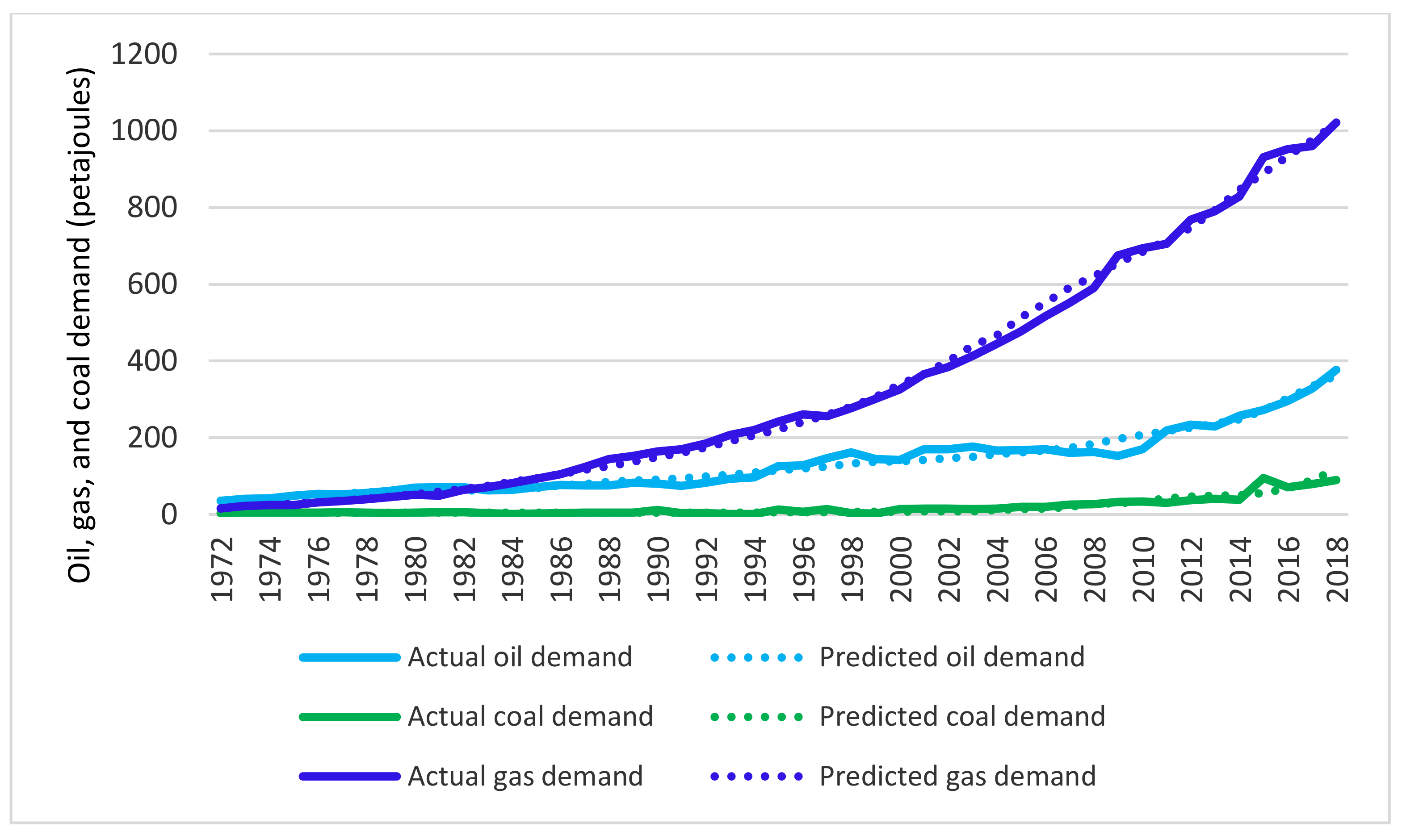
To check reliability of our forecast, using the parameter estimates of the OLS and SURE models, we first conducted in-sample forecasts for the 1972–2018 period and plotted these against the actual demand. Figure 4 compares the actual aggregate energy demand against the forecast demand from both the OLS models, and Figure 5 presents the forecast coal, gas, and oil demands generated using the SURE model parameters against the actual demands of these three energy sources. Both the figures show that the actual and forecast demands were almost identical, except for a few years showing minor differences. The differences were observed in years where the actual demand showed unusual trends, for instance in the case of aggregate demand in 2015.
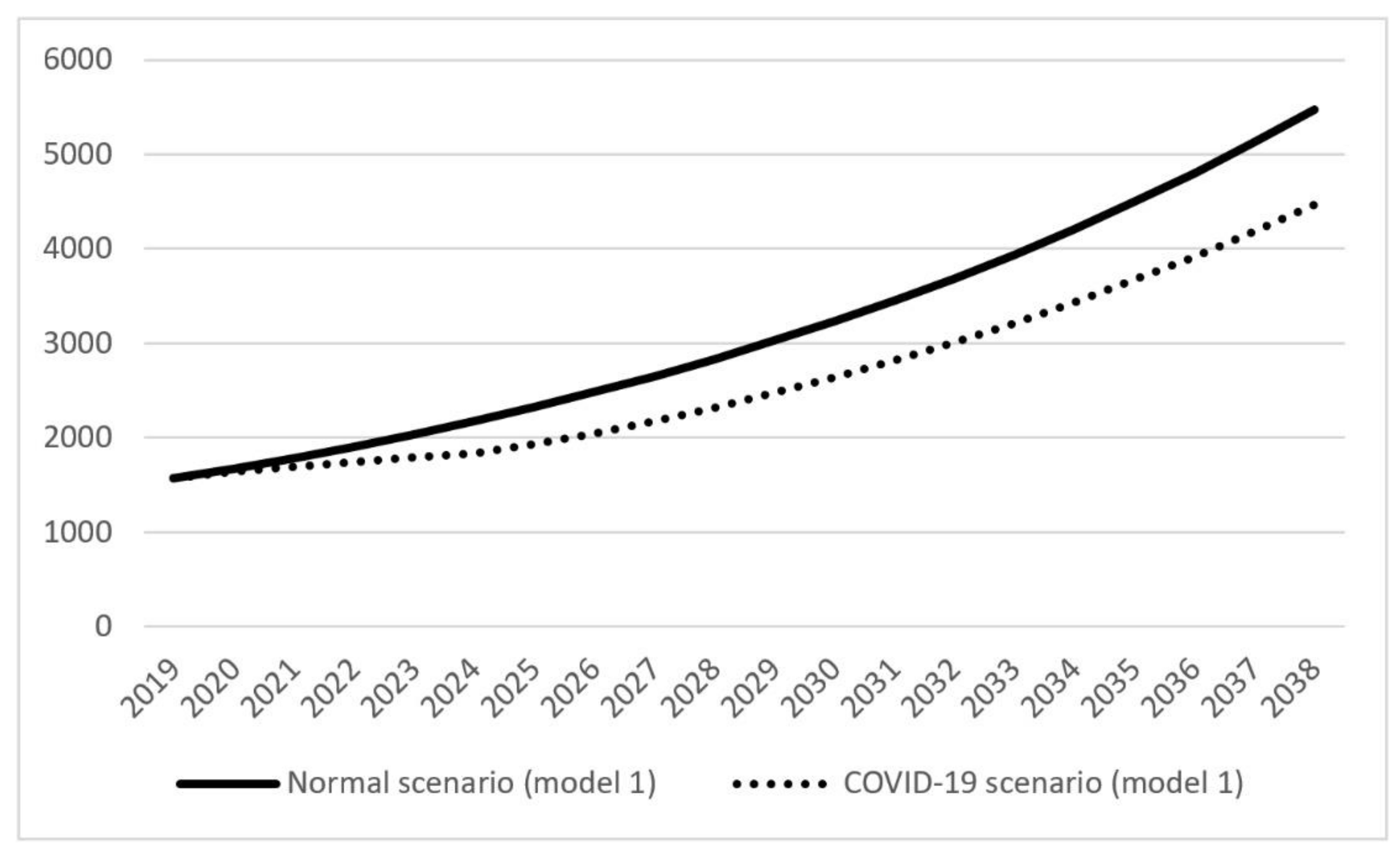
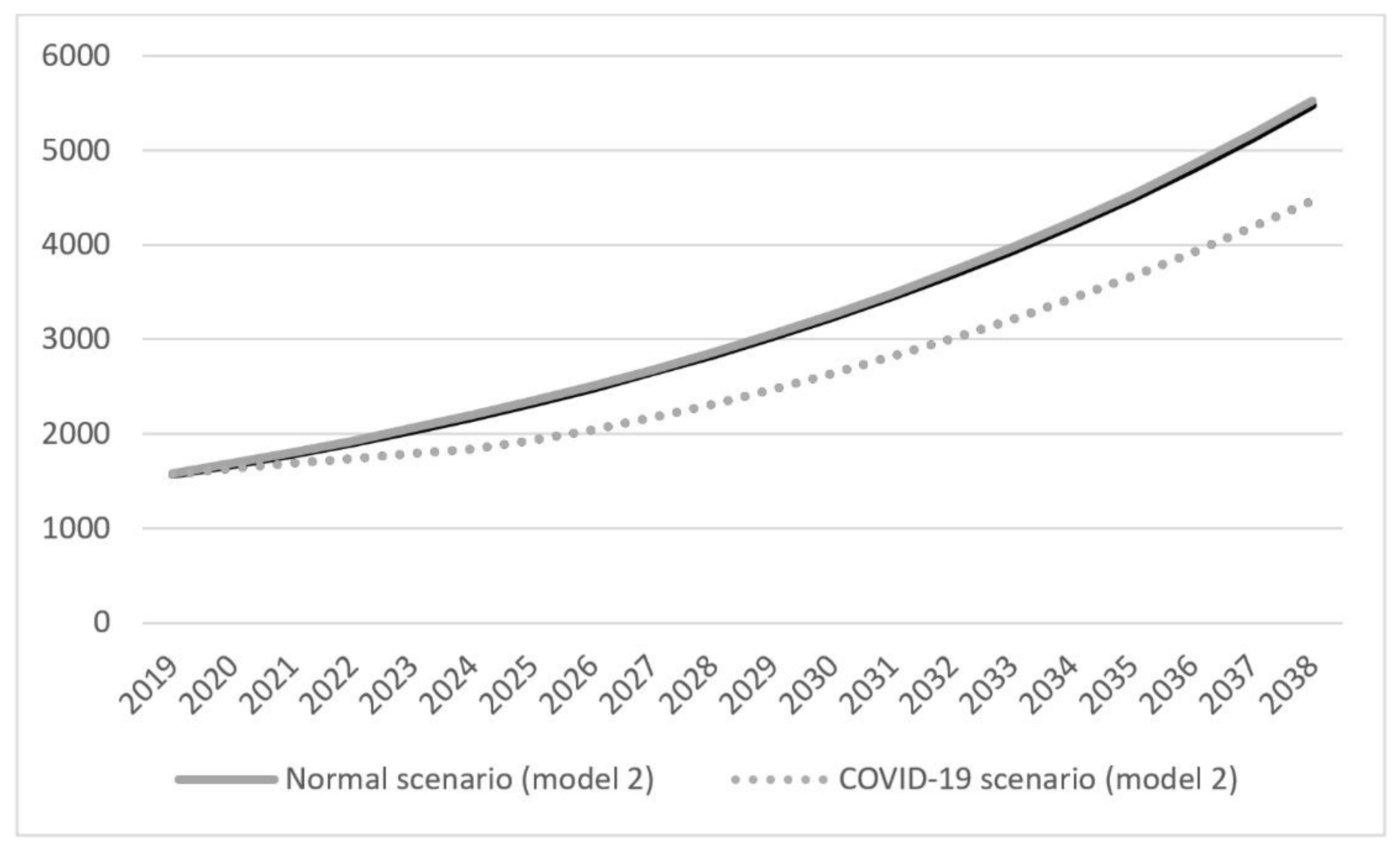
Figure 6 and Figure 7 present the aggregate energy demand in Bangladesh for the next two decades (2019–2038) based on forecasts from model 1 and model 2, respectively, whereas coal, gas, and oil demand are presented in Figure 8. Along with forecasts under the normal scenario, we also forecast considering possible effects of the COVID-19 pandemic on GDP. The aggregate demand forecast across models did not vary notably, rather as expected, although we observed a massive effect of COVID-19 on aggregate demand. Compared to a baseline scenario of 1487.31 petajoules of aggregate actual demand in 2018, demand in 2038 under the normal scenario in both the models was forecast to increase around 3.7-fold, a growth rate that is higher than what is forecast for many countries. For instance, during the period of 2017 to 2040, energy consumption in India, China, and in other Asian countries is expected to increase 2.56-, 1.28-, and 1.78-fold, respectively [46]. When the possible effect of COVID-19 was considered, demand was forecast to increase no more than 3-fold, which is at least around 23% less than that of the normal scenario.
Table 4 presents the results of the sensitivity analysis, i.e., the relative changes in total energy demand when we assumed additional changes in GDP and population growth rates. Compared to the business-as-usual scenario, demand was relatively high when we assumed Scenario 3, which had the higher GDP and population growth rates. Scenario 2, where the lowest GDP and population growth rates were assumed, resulted in the lowest deviation.
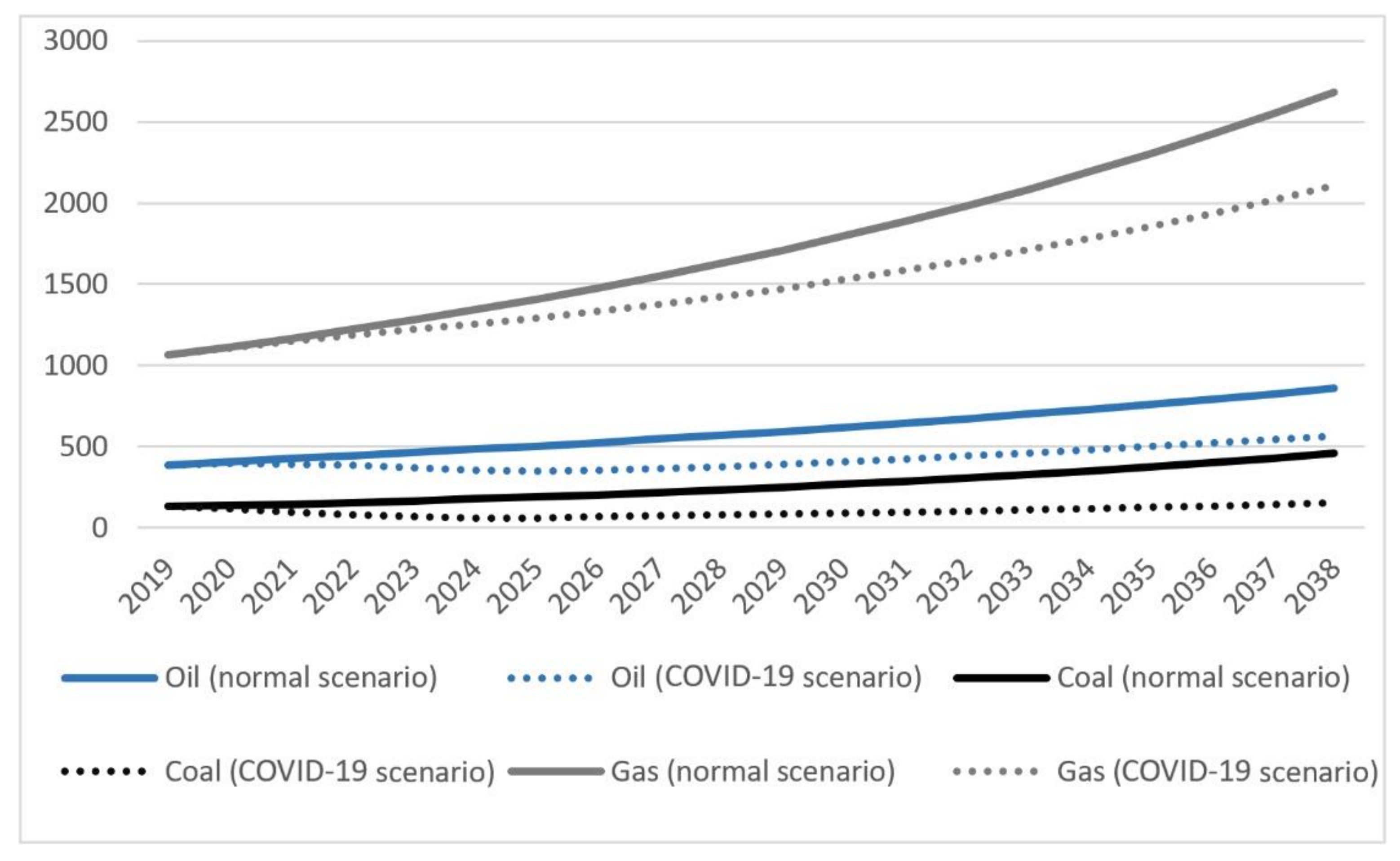
The forecast oil, coal, and gas demands in 2038 were 858.83 petajoules, 460.63 petajoules, and 2684.72 petajoules, which were 2.28, 5.16 and 2.63 times higher than those of 2018, respectively. Natural gas (67.05%) remained the major source, followed by oil (21.45%) and coal (11.50%). The demand increase was less pronounced when the possible effect of COVID-19 was considered; for instance, oil demand in 2038 was only 1.50 times higher. Coal demand faced the hardest hit and grew only 1.73-fold, which was around 66.47% lower than that of the normal scenario. Among the three energy sources, gas demand experienced the least effect. Nevertheless, gas demand was 21.44% lower than that in the normal scenario.
5. Discussion
The signs associated with the explanatory variables, at least those having significant effects, were in line with our expectations. The positive association between GDP/income and energy demand is well documented in the literature, though a consensus on the direction of causality is yet to be reached. While some have argued that energy demand contributes to increased GDP/income [27,47,48], many have argued that the causality is opposite [30,49] and some have argued for simultaneous causality [50,51]. Paul and Uddin [29] investigated this ambiguous relationship and revealed that output fluctuations drive energy demand in Bangladesh, and not the other way around. A similar direction of relationship was reported by Mazumder and Marathe [27] and Das et al. [23]. The robust effect of the income variable across the models, except in the equation for natural gas demand, revealed that growth in future GDP/income will be the major driver of energy demand in Bangladesh. Our estimated income elasticities for aggregate and oil demand were consistent with the literature wherein income elasticity for energy is inelastic, particularly in developing countries [52,53,54]. The very high income elasticity for coal is probably the outcome of government’s policy shift towards coal-based power plants. As already discussed in Section 2.2, due to reasons including the relatively lower coal price, less price volatility, and diversified sources, the government initiated several massive coal-based power plants during this millennium to overcome the gross power shortage. The GDP growth during this millennium helped the country to make the necessary investments. Such high income elasticity is not uncommon in the literature. Van Benthem and Romani [28], for instance, reported that income elasticity of energy could be high and increased with income, whereas Dhungel [55] estimated income elasticity of energy in Nepal to be as high as 3.04.
It is obvious that with a growing population, energy demand increases, which we observed for aggregate energy demand. However, we did not find coefficients on the population variable to be statistically significantly different from zero in any of the equations of the SURE model. This was similar to the findings of Wadud et al. [22] in the case of natural gas demand in Bangladesh, which they argued to be the consequence of large suppressed demand.
We did not observe the expected robust effect of price across models, though the elasticities were negative at least in models with significant effect. The negative own-price elasticity of weighted average price in model 1 and oil price in the oil demand equation were in line with the literature [52,56,57]. The statistically insignificant effect of energy price elasticities in most cases conflicts with our understanding about own- and cross-price elasticities, as was the experience of Wadud et al. [22] for natural gas demand in Bangladesh and Vu et al. [58] for electricity demand in Australia. We can offer three background reasons for this. First, for several reasons, energy prices in Bangladesh are highly subsidized. The low price makes consumers insensitive to price rises. The subsidy may make up for the increased cost. Here, the findings of van Benthem and Romani [28] are worth mentioning; they reported energy demand to be more sensitive to end-use price than to changes in international price. Second, overnight shifting from any energy source is not feasible, as the shift may require technical adjustments and costs. This was further confirmed by the highly significant effect of the lagged energy variable. This was particularly true for the cross-price elasticity. For instance, increased cost of CNG, which is widely used as a transportation fuel in Bangladesh, may discourage a new owner from investing to convert his/her vehicle to a natural-gas-powered one because of the high fixed cost associated with such a conversion. Those who have already converted may reduce their gas use to some extent, but are unlikely to give it up completely, since the gas price is still well below the petroleum price. Third, the very low per capita energy consumption in the country indicates that there is a large suppressed energy demand in Bangladesh. Under such circumstances, consumers are less likely to be concerned about costs and to make trade-offs in favor of cost to quantity.
Our forecasts show that Bangladesh will experience massive growth in energy demand. Therefore, ensuring an increasing supply of energy is critical for maintaining the country’s economic development process. This is particularly true since natural gas reserve in the country may run out in a decade or so if no additional reserves are found and the current production and extraction rate continues [59]. The drying out of the lone indigenous source will ultimately make the county dependent on imported oil, implying more and more budgetary pressure and more exposure to external market shocks. Ultimately, concerns about sustainability of the production system and global warming will have much higher stakes. The energy sector in the country is increasingly being subsidized, and it consumes more than half of the total budgetary subsidy of the government [60]. Though the government is continuing its subsidy policy for several good reasons, there is a long, ongoing, and unresolved debate concerning the efficiency and equity implications of this subsidy [61]. The very low energy efficiency in the country, from production to distribution, is a critical concern for the country [62,63]. A glimpse of hope for the country is that though the current contribution of renewable energy sources is not at all worth mentioning (less than 1% of total commercial energy), it can be promoted. The REN21 report predicted that from a coverage of merely 8% in 2017, all the households in Bangladesh will be under solar energy coverage by 2050 [64].
6. Future Energy Demand and Policy Changes
The forecasts reported in this study are based on the business-as-usual scenario. Since we are dealing with time-series data, changes in technology and related efficiency are already incorporated to some extent and the projections are based on the trend observed. However, this fails to incorporate future structural changes brought by shifts in policy regime. For instance, understanding the importance of environmental sustainability in 2021, Bangladesh updated the Nationally Determined Contributions (NDCs) which aim to reduce GHG emissions by 27.56 Mt CO2e, which is 6.73% below the level of emission that would be generated from the projected business-as-usual scenario. The energy sector is targeted to make the largest contribution (95.4%) in this emission reduction. However, if the current trend in energy consumption continues, the demands for oil, coal, and gas for energy purposes will increase around 1.5-, 1.9-, and 1.5-fold, respectively. Therefore, the set targets require drastic policy interventions in order to increase energy efficiency and replace nonrenewable conventional energy sources with sustainable renewable energy sources.
Though the target has been set for emission reduction, the mechanisms and strategies are yet to be designed in detail by the government. The NDC 2021 report of the Ministry of Environment, Forest, and Climate Change mentioned only guiding principles, which include a wide range of strategies ranging from capacity development, monitoring and ensuring transparency, and other institutional measures. To what extent Bangladesh is capable of achieving this ambitious emission reduction target is yet to be explored in the future.
7. Conclusions and Policy Implications
The study first aimed at identifying the determinants of oil, natural gas, coal, and aggregate fuel demand in Bangladesh using the longest possible time-series, covering a 47 year period (1972–2018), and then forecasting energy demand for the period of 2019 to 2038 under both business-as-usual and ongoing COVID-19 pandemic scenarios. The results reveal that the aggregate demand for energy will increase by 400% by 2038 under the business-as-usual scenario, whereas accounting for the projected effect of COVID-19 on the economy will suppress the increase in demand for energy to 300% of its existing level. Similarly, demand for all the three major energy sources will increase, within which the highest increase in demand will occur for coal (3.94-fold), followed by gas (2.64-fold) and oil (2.37-fold). While, GDP and lagged energy demand had the most robust effect across all models, we did not see much effect of own and cross prices of energy sources on energy demand.
As the economy of Bangladesh grows, the demand for energy will continue to grow, but several concerns remain. This is because natural gas, the only indigenous and the major energy source for Bangladesh, is expected to run out within the next two decades. With a decline in the supply of natural gas from internal sources and the growing demand for energy over time, the country will be more exposed to the external shocks and volatility of international energy markets. In addition, the efficiency and equity effects of the existing energy subsidy, the volume of which is continuously increasing, need to be evaluated.
Based on the findings of the study, the following policy implications can be formulated. The policy directions are geared towards two strategic pathways: (a) building the capacity of commercial energy generation by undertaking new power installations with the required safety and security measures, as well as removing inefficiencies in production and generation of energy and its services; and (b) shifting away from traditional energy sources towards renewable and green energy sources, although there may be challenges. First, the main thrust should be to promote use of renewable and green energy sources. This is because the country will lose its advantage of natural gas supply from its own source in the near future. The existing thrust in the plan to meet the challenge of increasing demand with coal and nuclear power plants should be scrutinized on sustainability and safety grounds, as both are potentially hazardous sources of energy production unless strict safety measures are enforced effectively. The government’s claim of safety and security assurances of these proposed coal and nuclear power plants are doubtful and there are concerns about a lack of transparency of the process. Second, a remarkable 43% of the total retail electricity is consumed at the household level [65], where the use of renewable and green energy sources such as solar power could be a viable option, which in turn could curb the rise in demand for fossil fuels. The costs of renewable energy sources have fallen by 95% from their initial level about a decade ago, and these technologies are relatively much cheaper to install now. Additionally, renewable energy technologies have substantially improved over time, and have become more energy efficient and a reliable source of power as compared to their predecessors. The government can follow strategies undertaken in developed countries to not only encourage solar power and other renewable installations by individuals and organizations, but also buy-in of solar power supply to the national grid, which will create a market for energy trading within the economy. Currently, the government imposes the condition that all new private developments in the metropolitan areas must use renewable sources, which should be rolled out nationwide. The third point is to improve the efficiency of both production and distribution of energy. Bangladesh has a reputation of being one of the most inefficient producers and distributers of energy and its services. The government should pay serious attention to resolving this inefficiency issue, which not only increases the costs of producing energy services but also wastes produced energy, by focusing on technological solutions as well as institutional reforms. Fourth, although the existing level of subsidy in the energy sector cannot be withdrawn fully because of its serious adverse consequences on poverty and the development trajectory, the government can redesign its subsidy strategy using market-based approaches, which will compel consumers to divert towards either energy efficiency or use of environmentally friendly energy technologies. Finally, we also echo the NDC (2021) report asking for regular quantitative study to monitor Bangladesh’s success in achieving reduction in emission targets.
Author Contributions
Conceptualization, S.R. and A.R.A.; methodology, S.R. and A.R.A.; formal analysis, A.R.A.; data curation, A.R.A.—original draft preparation, S.R.—review and editing, S.R.; supervision, S.R. Both authors have read and agreed to the published version of the manuscript.
Funding
This research received no external funding.
Institutional Review Board Statement
Not Applicable.
Informed Consent Statement
Not applicable.
Conflicts of Interest
The authors declare no conflict of interest.
Appendix A
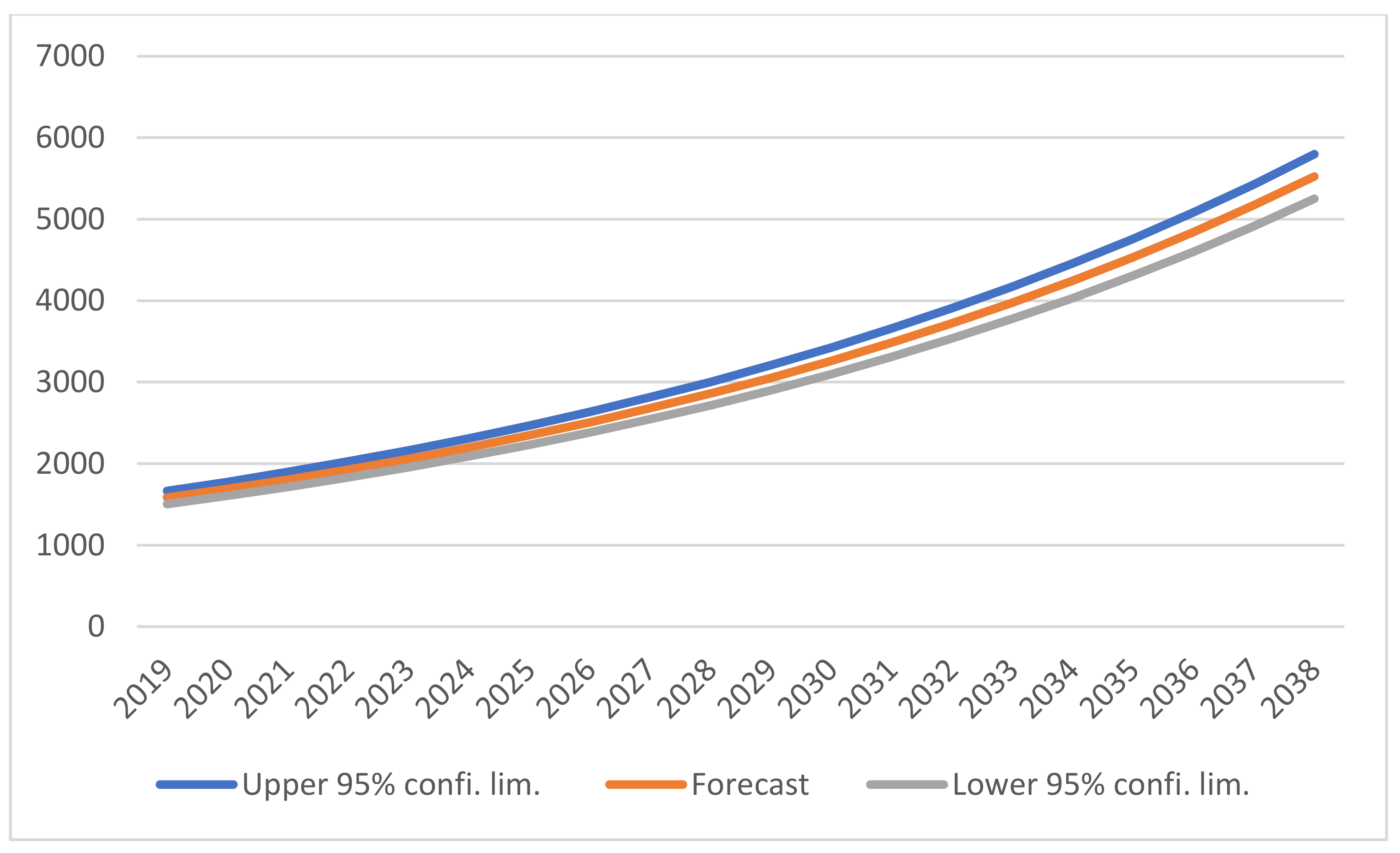
Figure A1.
Forecast total energy demand for model 1 and upper and lower confidence limit at 95% (model 1).
Figure A1.
Forecast total energy demand for model 1 and upper and lower confidence limit at 95% (model 1).

Figure A2.
Forecast total energy demand for model 1 and upper and lower confidence limit at 95% (model 2).
Figure A2.
Forecast total energy demand for model 1 and upper and lower confidence limit at 95% (model 2).

References
- EIA. Energy Overview. U.S. Department of Energy. Available online: https://www.eia.gov/totalenergy/data/browser/#/?f=A&start=1949&end=2019&charted=4-6-7-14 (accessed on 4 May 2020).
- Kibria, A.; Akhundjanov, S.B.; Oladi, R. Fossil fuel share in the energy mix and economic growth. Int. Rev. Econ. Financ. 2019, 59, 253–264. [Google Scholar] [CrossRef]
- IEA. World Energy Outlook 2007; International Energy Agency: Paris, France, 2007. [Google Scholar]
- ADB. Asian Development Outlook 2013 Update: Governance and Public Service Delivery; Asian Development Bank: Manila, Philippine, 2013. [Google Scholar]
- CNPC. World and China Energy Outlook 2050; CNPC Economics and Technology Research Institute: Beijing, China, 2018. [Google Scholar]
- EIA. Bangladesh 2017 Primary Energy Data in Quadrillion Btu. Available online: https://www.eia.gov/international/overview/country/BGD (accessed on 5 May 2020).
- World Bank. Industrialization Intensity Index, TCdata360, World Bank. Available online: https://tcdata360.worldbank.org/indicators/mva.ind.int?country=BGD&indicator=3793&viz=line_chart&years=1990,2014 (accessed on 4 May 2020).
- Soytas, U.; Sari, R. Energy consumption and GDP: Causality relationship in G-7 countries and emerging markets. Energy Econ. 2003, 25, 33–37. [Google Scholar] [CrossRef]
- Trading Economics. Available online: https://tradingeconomics.com/bangladesh/energy-imports-net-percent-of-energy-use-wb-data.html (accessed on 14 May 2020).
- Regnier, E. Oil and energy price volatility. Energy Econ. 2007, 29, 405–427. [Google Scholar] [CrossRef]
- Awerbuch, S.; Sauter, R. Exploiting the oil-GDP effect to support renewables deployment. Energy Policy 2006, 34, 2805–2819. [Google Scholar] [CrossRef]
- Baldwin, R.; di Mauro, B.W. Economics in the Time of COVID-19; Centre for Economic Policy Research (CERP): London, UK, 2020. [Google Scholar]
- Yilmazkuday, H. Coronavirus Disease 2019 and the Global Economy. Available online: https://papers.ssrn.com/sol3/papers.cfm?abstract_id=3554381; (accessed on 20 September 2020).
- EIA. Pakistan 2017 Primary Energy Data in Quadrillion Btu. Available online: https://www.eia.gov/international/overview/country/PAK (accessed on 7 May 2020).
- Our World in Data. Available online: https://ourworldindata.org/#entries (accessed on 2 February 2020).
- Islam, S.; Khan, M.Z. A review of energy sector of Bangladesh. Energy Procedia 2017, 110, 611–618. [Google Scholar] [CrossRef]
- BBS. Statistical Year Book of Bangladesh 2018; Bangladesh Bureau of Statistics: Dhaka, Bangladesh, 2019.
- Suganthi, L.; Samuel, A.A. Energy models for demand forecasting—A review. Renew. Sustain. Energy Rev. 2012, 16, 1223–1240. [Google Scholar] [CrossRef]
- Ghalehkhondabi, I.; Ardjmand, E.; Weckman, G.R.; Young, W.A. An overview of energy demand forecasting methods published in 2005–2015. Energy Syst. 2017, 8, 411–447. [Google Scholar] [CrossRef]
- Kandananond, K. Forecasting electricity demand in Thailand with an artificial neural network approach. Energies 2011, 22, 1246–1257. [Google Scholar] [CrossRef]
- Xie, N.M.; Yuan, C.Q.; Yang, Y.J. Forecasting China’s energy demand and self-sufficiency rate by grey forecasting model and Markov model. Int. J. Electr. Power Energy Syst. 2015, 66, 1–8. [Google Scholar] [CrossRef]
- Wadud, Z.; Dey, H.S.; Kabir, M.A.; Khan, S.I. Modeling and forecasting natural gas demand in Bangladesh. Energy Policy 2011, 39, 7372–7380. [Google Scholar] [CrossRef] [Green Version]
- Das, A.; McFarlane, A.A.; Chowdhury, M. The dynamics of natural gas consumption and GDP in Bangladesh. Renew. Sustain. Energy Rev. 2013, 22, 269–274. [Google Scholar] [CrossRef]
- Mondal, M.A.H.; Boie, W.; Denich, M. Future demand scenarios of Bangladesh power sector. Energy Policy 2010, 38, 7416–7426. [Google Scholar] [CrossRef]
- Debnath, K.B.; Mourshed, M.; Chew, S.P.K. Modelling and forecasting energy demand in rural households of Bangladesh. Energy Procedia 2015, 75, 2731–2737. [Google Scholar] [CrossRef] [Green Version]
- Kabir, G.; Sumi, R. Integrating fuzzy Delphi method with artificial neural network for demand forecasting of power engineering company. Manag. Sci. Lett. 2012, 2, 1491–1504. [Google Scholar] [CrossRef]
- Mozumder, P.; Marathe, A. Causality relationship between electricity consumption and GDP in Bangladesh. Energy Policy 2007, 35, 395–402. [Google Scholar] [CrossRef]
- Van Benthem, A.; Romani, M. Fuelling growth: What drives energy demand in developing countries? Energy J. 2009, 30, 91–114. [Google Scholar] [CrossRef]
- Paul, B.P.; Uddin, G.S. Energy and output dynamics in Bangladesh. Energy Econ. 2011, 33, 480–487. [Google Scholar] [CrossRef]
- Rahman, S. Energy demand perspectives in Bangladesh: 1992/93-2019/20 AD. Bangladesh J. Agric. Econs. 1998, 21, 39–57. [Google Scholar]
- Ibrahim, I.B. Hurst, C. Estimating energy and oil demand functions. Energy Econ. 1990, 13, 93–102. [Google Scholar] [CrossRef]
- Tzeng, G.H. Modeling energy demand and socioeconomic development of Taiwan. Energy J. 1989, 10, 133–151. [Google Scholar] [CrossRef]
- Kaboudan, M.A.; Liu, Q.W. Forecasting quarterly US demand for natural gas. Inf. Technol. Econ. Manag. 2004, 2, 1–14. [Google Scholar]
- Gujarati, D.N. Basic Econometrics, 5th ed.; Tata McGraw-Hill Education: New Delhi, India, 2009. [Google Scholar]
- Wooldridge, J.M. Introductory Econometrics: A Modern Approach, 6th ed.; Cengage Learn: Mason, OH, USA, 2015. [Google Scholar]
- Liew, V.K.S. Which lag length selection criteria should we employ? Econ. Bull. 2004, 3, 1–9. [Google Scholar]
- Zellner, A. An efficient method of estimating seemingly unrelated regressions and tests for aggregation bias. J. Am. Stat. Assoc. 1962, 57, 348–368. [Google Scholar] [CrossRef]
- Zellner, A.; Huang, D.S. Further properties of efficient estimators for seemingly unrelated regression equations. Int. Econ. Rev. 1962, 3, 300–313. [Google Scholar] [CrossRef]
- Zellner, A. Estimators for seemingly unrelated regression equations: Some exact finite sample results. J. Am. Stat. Assoc. 1963, 58, 977–992. [Google Scholar] [CrossRef]
- Cameron, A.C.; Trivedi, P.K. Microeconometrics Using Stata, Revised Edition; Stata Press: College Station, TX, USA, 2010. [Google Scholar]
- StataCorp. Stata Statistical Software: Release 14; StataCorp LP: College Station, TX, USA, 2015. [Google Scholar]
- Breusch, T.S.; Pagan, A.R. The Lagrange multiplier test and its applications to model specification in econometrics. Rev. Econ. Stud. 1980, 47, 239–253. [Google Scholar] [CrossRef]
- Kilian, L. Not all oil price shocks are alike: Disentangling demand and supply shocks in the crude oil market. Am. Econ. Rev. 2009, 99, 1053–1069. [Google Scholar] [CrossRef] [Green Version]
- World Economic Outlook. Available online: https://www.imf.org/external/datamapper/NGDP_RPCH@WEO/ISR?year=2021 (accessed on 13 June 2020).
- Global Economic Prospects—Forecasts. Available online: https://data.worldbank.org/country/BD (accessed on 13 June 2020).
- BP. BP Energy Outlook 2019; British Petroleum: London, UK, 2019. [Google Scholar]
- Aqeel, A.; Butt, M.S. The relationship between energy consumption and economic growth in Pakistan. Asia Pac. Dev. J. 2001, 8, 101–110. [Google Scholar]
- Shiu, A.; Lam, L.P. Electricity consumption and economic growth in China. Energy Policy 2004, 32, 47–54. [Google Scholar] [CrossRef]
- Ghosh, S. Electricity consumption and economic growth in India. Energy Policy 2002, 30, 125–129. [Google Scholar] [CrossRef]
- Morimoto, R.; Hope, C. The impact of electricity supply on economic growth in Sri Lanka. Energy Econ. 2004, 26, 77–85. [Google Scholar] [CrossRef]
- Chen, S.T.; Kuo, H.I.; Chen, C.C. The relationship between GDP and electricity consumption in 10 Asian countries. Energy Policy 2007, 35, 2611–2621. [Google Scholar] [CrossRef]
- Gately, D.; Huntington, H.G. The asymmetric effects of changes in price and income on energy and oil demand. Energy J. 2002, 23, 19–55. [Google Scholar] [CrossRef] [Green Version]
- Webster, M.; Paltsev, S.; Reilly, J. Autonomous efficiency improvement or income elasticity of energy demand: Does it matter? Energy Econ. 2008, 30, 2785–2798. [Google Scholar] [CrossRef]
- Lee, C.C.; Lee, J.D. A panel data analysis of the demand for total energy and electricity in OECD countries. Energy J. 2010, 31, 1–23. [Google Scholar] [CrossRef]
- Dhungel, K.R. Income and price elasticity of the demand for energy: A macro-level empirical analysis. Pac. Asian J. Energy 2003, 13, 73–84. [Google Scholar]
- Graham, D.J.; Glaister, S. The demand for automobile fuel: A survey of elasticities. J. Transp. Econ. Policy 2002, 36, 1–26. [Google Scholar]
- Wadud, Z.; Graham, D.J.; Noland, R.B. Gasoline demand with heterogeneity in household responses. Energy J. 2010, 31, 47–74. [Google Scholar] [CrossRef] [Green Version]
- Vu, D.H.; Muttaqi, K.M.; Agalgaonkar, A.P. A variance inflation factor and backward elimination based robust regression model for forecasting monthly electricity demand using climatic variables. Appl. Energy 2015, 140, 385–394. [Google Scholar] [CrossRef] [Green Version]
- Shetol, M.H.; Rahman, M.M.; Sarder, R.; Hossain, M.I.; Rhidoy, F.K. Present status of Bangladesh gas fields and future development: A review. J. Nat. Gas Geosci. 2019, 4, 347–354. [Google Scholar] [CrossRef]
- Amin, S. The Macroeconomics of Energy Price Shocks and Electricity Market Reforms: The Case of Bangladesh. Ph.D. Thesis, Durham University, Durham, UK, 2015. [Google Scholar]
- Timilsina, G.R.; Pargal, S.; Tsigas, M.; Sahin, S. How Much Would Bangladesh Gain from the Removal of Subsidies on Electricity and Natural Gas? In Policy Research; Working Paper 8677; World Bank: Washington, DC, USA, 2018. [Google Scholar]
- Gunatilake, H.; Ronald-Holst, D. Energy Policy Options for Sustainable Development in Bangladesh. In ADB Economics; Working Paper Series 359; Asian Development Bank: Manila, Philippine, 2013. [Google Scholar]
- SREDA; PD. Energy Efficiency and Conservation Master Plan up to 2030; Ministry of Power, Energy and Mineral Resources, Government of the People’s Republic of Bangladesh: Dhaka, Bangladesh, 2015.
- REN 21. Available online: https://www.ren21.net/ (accessed on 7 June 2020).
- BPDC. Annual Report 2018–2019; Bangladesh Power Development Corporation: Dhaka, Bangladesh, 2019. [Google Scholar]
Figure 1.
Per capita energy use (tonne of oil equivalent per capita).

Figure 2.
Total primary energy consumption by conventional sources (petajoule) in Bangladesh.

Figure 3.
Proportion of primary energy consumption by conventional sources (%) in Bangladesh.

Figure 4.
Comparison of actual vs. predicted total energy demand (petajoules).

Figure 5.
Comparison of actual vs. predicted oil, coal, and gas demand (petajoules).

Figure 6.
Forecast total energy demand for model 1 (petajoules). Note: We calculated the ex ante errors (i.e., upper and lower limits of confidence interval) for the forecast total energy demand under the business-as-usual scenario. In percentage terms, the maximum deviation was consistent and ranged from 3.6 to 3.7% for the upper level and −3.7 to −3.6% for the lower level. The trend graphs are presented in Appendix A Figure A1.

Figure 7.
Forecast total energy demand for model 2 (petajoules). Note: We calculated the ex ante errors (i.e., upper and lower limits of confidence interval) for the for the forecast total energy demand under the business-as-usual scenario. In percentage terms, the maximum deviation was consistent and ranged within 5.0 to 5.1% for the upper level and −5.1 to −5.0% for the lower level. The trend graphs are presented in Appendix A Figure A2.

Figure 8.
Forecast oil, coal, and gas demand (petajoules).


Table 1.
Growth rate (%) in per capita energy consumption (tonne of oil equivalent).
| Period | Bangladesh | China | India | Pakistan | Sri Lanka |
|---|---|---|---|---|---|
| 1972–2000 | 5.02 | 3.60 | 3.58 | 3.38 | 3.02 |
| 2001–2018 | 4.76 | 5.40 | 4.15 | 1.22 | 2.84 |
| Whole period | 4.81 | 4.58 | 3.55 | 2.54 | 3.64 |
Note: The annual exponential growth rate is the parameter in .
Table 2.
Growth rate (%) in total energy consumption in Bangladesh (petajoule).
| Period | Oil | Natural Gas | Coal | Total |
|---|---|---|---|---|
| 1972–2000 | 4.49 | 10.64 | 0.44 | 7.45 |
| 2001–2018 | 4.58 | 6.23 | 11.35 | 5.99 |
| Whole period | 4.34 | 8.67 | 6.69 | 6.84 |
Table 3.
Parameter estimates and model diagnostics for energy demand by source.
| Regressors | Aggregate Energy Demand (OLS Model) | Energy Demand by Source (SURE Model) a | |||
|---|---|---|---|---|---|
| Model 1 | Model 2 | Oil | Coal | Gas | |
| GDP (USD per capita) | 0.307 *** (0.095) | 0.334 *** (0.117) | 0.356 *** (0.148) | 2.250 *** (0.869) | 0.082 (0.086) |
| Population | 1.586 *** (0.450) | 1.513 *** (0.473) | 0.284 (0.187) | −0.339 (0.898) | 0.105 (0.525) |
| Weighted price | −0.029 * (0.016) | -- | -- | -- | -- |
| Oil price | -- | −0.021 (0.026) | −0.075 ** (0.037) | 0.037 (0.034) | 0.011 (0.028) |
| Coal price | -- | 0.011 (0.032) | 0.037 (0.034) | 0.327 (0.314) | −0.048 (0.039) |
| Gas price | -- | −0.010 (0.022) | 0.011 (0.028) | −0.048 (0.039) | 0.027 (0.027) |
| Lag 1 of independent variable | 0.350 ** (0.164) | 0.360 ** (0.168) | 0.897 *** (0.140) | 0.374 *** (0.144) | 0.536 *** (0.134) |
| Lag 2 of independent variable | 0.068 (0.141) | 0.066 (0.149) | −0.224 (0.146) | −0.166 (0.144) | 0.376 *** (0.127) |
| Constant | −8.302 *** (2.561) | −7.264 *** (2.639) | 4.806 * (2.551) | 27.061 ** (12.989) | 0.999 (5.252) |
| Hypothesis testing and goodness of fit for the OLS model | |||||
| Jarque-Bera test for normality . | 0.690 | 0.763 | -- | -- | -- |
| Breusch-Pagan LM statistic | |||||
| (1) | 0.379 | 0.001 | -- | -- | |
| p-value | 0.538 | 0.98 | -- | -- | -- |
| Stationarity test | |||||
| Durbin-Watson d-statistic | 1.887 (6, 45) | 1.902 (8, 45) | -- | -- | -- |
| Breusch-Godfrey LM test for autocorrelation | |||||
| (1) | 0.031 | 0.013 | -- | -- | |
| Prob > | 0.859 | 0.908 | -- | -- | -- |
| 0.998 | 0.998 | -- | -- | -- | |
| Hypothesis testing and goodness of fit for the SURE model | |||||
| Breusch-Pagan test of independence | |||||
| (3) | -- | -- | 7.476 | ||
| p-value | -- | -- | 0.058 | ||
| Root mean square error (RMSE) | -- | -- | 0.082 | 0.553 | 0.054 |
| Pseudo | -- | -- | 0.983 | 0.811 | 0.998 |
| F-Stat | -- | -- | 368.99 *** | 27.97 *** | 3241.62 *** |
| N | 45 | 45 | 45 | 45 | 45 |
Note: a Restrictions imposed: and for all and . *, **, and *** represent significance levels of 1%, 5%, and 10%, respectively. Figures in parentheses are standard errors.
Table 4.
Sensitivity analysis: % changes in forecast total energy demand under different alternative scenarios compared to actual demand.
Table 4.
Sensitivity analysis: % changes in forecast total energy demand under different alternative scenarios compared to actual demand.
| Year | Model 1 | Model 2 | ||||||
|---|---|---|---|---|---|---|---|---|
| Scenario 1 | Scenario 2 | Scenario 3 | Scenario 4 | Scenario 1 | Scenario 2 | Scenario 3 | Scenario 4 | |
| 2019 | 4.82 | 3.88 | 5.17 | 4.22 | 4.47 | 3.58 | 4.85 | 3.95 |
| 2024 | 7.93 | 6.29 | 8.54 | 6.88 | 8.00 | 6.41 | 8.67 | 7.07 |
| 2029 | 8.03 | 6.36 | 8.64 | 6.96 | 8.11 | 6.50 | 8.79 | 7.16 |
| 2034 | 8.03 | 6.36 | 8.64 | 6.96 | 8.11 | 6.50 | 8.79 | 7.17 |
| 2038 | 8.03 | 6.36 | 8.64 | 6.96 | 8.11 | 6.50 | 8.79 | 7.17 |
Publisher’s Note: MDPI stays neutral with regard to jurisdictional claims in published maps and institutional affiliations. |
© 2021 by the authors. Licensee MDPI, Basel, Switzerland. This article is an open access article distributed under the terms and conditions of the Creative Commons Attribution (CC BY) license (https://creativecommons.org/licenses/by/4.0/).
Share and Cite
MDPI and ACS Style
Anik, A.R.; Rahman, S. Commercial Energy Demand Forecasting in Bangladesh. Energies 2021, 14, 6394. https://doi.org/10.3390/en14196394
AMA Style
Anik AR, Rahman S. Commercial Energy Demand Forecasting in Bangladesh. Energies. 2021; 14(19):6394. https://doi.org/10.3390/en14196394
Chicago/Turabian StyleAnik, Asif Reza, and Sanzidur Rahman. 2021. "Commercial Energy Demand Forecasting in Bangladesh" Energies 14, no. 19: 6394. https://doi.org/10.3390/en14196394
Note that from the first issue of 2016, this journal uses article numbers instead of page numbers. See further details here.