
Design of Feedback Control Strategies in a Plant-Wide Wastewater Treatment Plant for Simultaneous Evaluation of Economics, Energy Usage, and Removal of Nutrients


Abstract
:1. Introduction
2. Materials and Methods
2.1. Influent Data
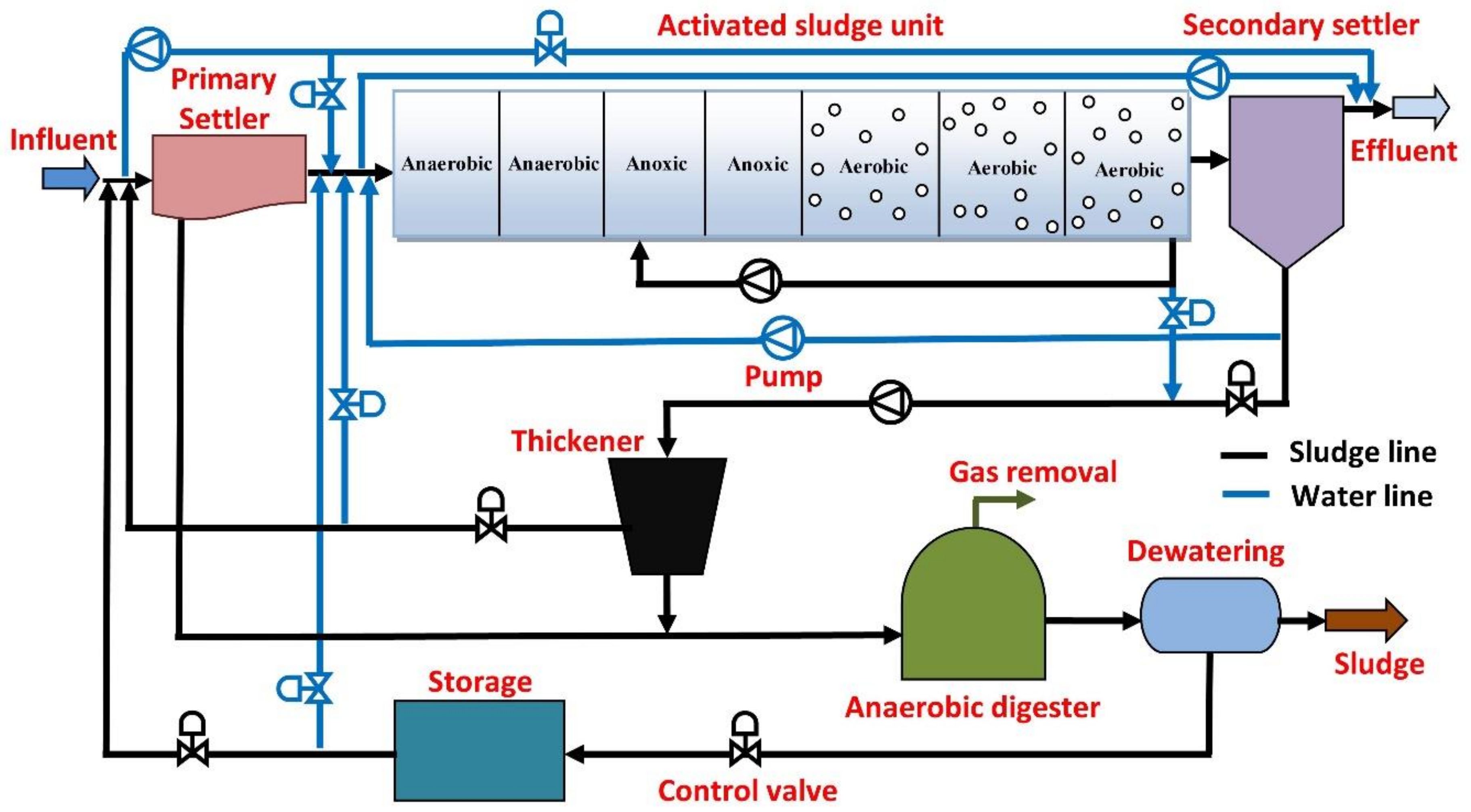
2.2. Model Scenario
2.3. Plant-Wide Assessment Criteria
2.3.1. Effluent Quality Index
2.3.2. Operational Cost Index (OCI)
3. Control Approaches
3.1. Design of Proportional-Integral (PI) Controller
3.2. Design of Model Predictive Controller (MPC)
3.3. Design of Fuzzy-Logic Controller (FLC)
4. Results and Discussion
4.1. PI Control (2 Loops)
- NO loop: KP = 0.000026144, τp = 0.012515, and θd = 0.000875.
- DO loop: KP = 0.04538, τi = 0.010085, and θd = 0.
4.2. PI Control (One Loop)
4.3. Ammonia-Based Aeration Control (ABAC) Approach
4.3.1. PI-MPC Control Strategy
4.3.2. PI-Fuzzy Control Strategy
- If SNH level is “low”, then SO level is “low”
- If SNH level is “high”, then SO level is “high”
- If SNH level is “medium”, then SO level is “medium”
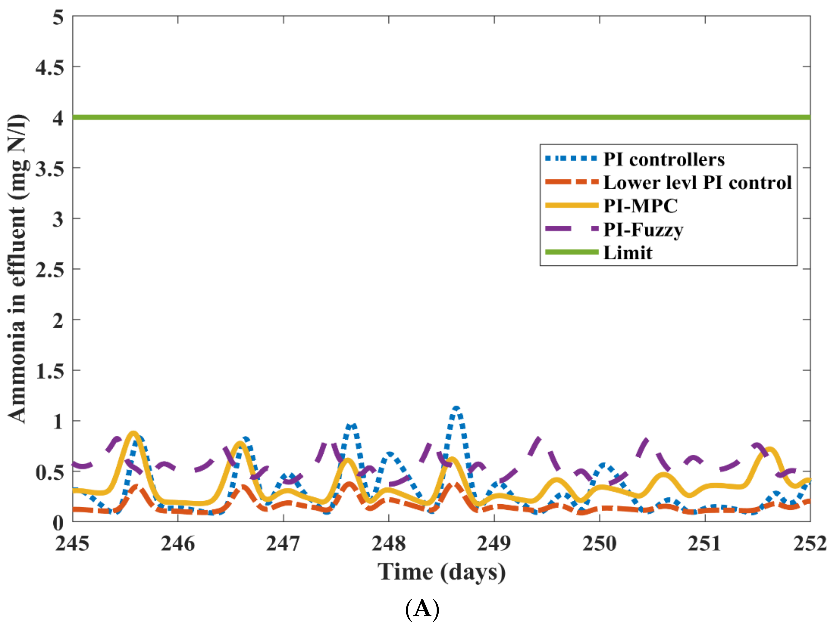
4.4. Comparison of Four Control Design Frameworks on BSM2-P
4.5. Summary of Previous and Present Studies on BSM2-P
5. Conclusions
Supplementary Materials
Author Contributions
Funding
Data Availability Statement
Acknowledgments
Conflicts of Interest
Nomenclature
| AE | Aeration Energy (Kwh/d) |
| ASM1 | Activated Sludge Model No.1 |
| ASM2 | Activated Sludge Model No.2 |
| ASM2d | Activated Sludge Model No.2d |
| ASM3 | Activated Sludge Model No.3 |
| BOD5 | Biological Oxygen Demand |
| COD | Chemical Oxygen Demand |
| DO | Dissolved Oxygen |
| EQI | Effluent Quality Index |
| IQI | Influent Quality Index |
| K | Proportional gain |
| KLa | Oxygen transfer coefficient |
| TN | Total Nitrogen |
| TKN | Total Kjeldahl Nitrogen |
| TSS | Total suspended solids |
| NO | Nitrate |
| P | Phosphorus |
| PE | Pumping Energy (kWh/d) |
| KUt | Pollutant load corresponding to component |
| Qo | Influent flow rate (m3/d) |
| Qintr | Internal recycle flow rate (m3/d) |
| Qr | Return sludge flow rate (m3/d) |
| Qw | Waste sludge flow rate (m3/d) |
| SA | Fermentation products (g COD/m3) |
| SF | Readily biodegradable organic substrate |
| SHCO | Alkalinity of the waste water (HCO3/m3) |
| SI | Inert soluble organic material (g COD/m3) |
| SNH | Ammonium and ammonia nitrogen (g N/m3) |
| SNO | Nitrate and nitrite nitrogen (g N/m3) |
| SN2 | Dinitrogen (g N/m3) |
| SPO4 | Inorganic soluble phosphate (g P/m3) |
| SS | Readily biodegradable organic substrate (g COD/m3) |
| to | Start time |
| tf | End time |
| BODef | Total BOD concentration |
| CODef | Total COD concentration |
| SNO | Nitrate concentration |
| SPorg | Total N concentration |
| SPinorg | Total phosphorus concentration |
| TKN | Total organic N concentration |
| WWTP | Wastewater Treatment Plant |
| XA | Nitrifying organisms (g COD/m3) |
| XH | Heterotrophic organisms (g COD/m3) |
| XI | Inert particulate organic material (g COD/m3) |
| XS | Slowly biodegradable substrates (g COD/m3) |
| XPAO | Poly accumulating organisms (g COD/m3) |
| XPHA | Cell internal storage product of PAO’S (g COD/m3) |
| XPP | Polyphosphate (g P/m3) |
| XSTO | Cell inner storage product of heterotopy |
| XTSS | Suspended solids (g SS/m3) |
References
- Matejczyk, M.; Ofman, P.; Dąbrowska, K.; Świsłocka, R.; Lewandowski, W. The study of biological activity of transformation products of diclofenac and its interaction with chlorogenic acid. J. Environ. Sci. 2020, 91, 128–141. [Google Scholar] [CrossRef] [PubMed]
- Solon, K. Extending Wastewater Treatment Process Models for Phosphorus Removal and Recovery: A Framework for Plant-Wide Approach of Phosphorus, Sulfur and Iron. Ph.D. Thesis, Lund University, Sweden, 2017. [Google Scholar]
- Asadi, A.; Verma, A.; Yang, K.; Mejabi, B. Wastewater treatment aeration process optimization: A data mining approach. J. Environ. Manag. 2017, 203, 630–639. [Google Scholar] [CrossRef] [PubMed]
- Olsson, G.; Newell, B. Wastewater Treatment Systems: Modelling, Diagnosis and Control; IWA Publishing: London, UK, 1999. [Google Scholar]
- Henze, M.; Gujer, W.; Mino, T.; van Loosdrecht, M.C.M. Activated Sludge Models ASM1, ASM2, ASM2d, and ASM3; IWA Scientific and Technical Report, No. 9; IWA Publishing: London, UK, 2000. [Google Scholar]
- Rieger, L.; Koch, G.; Kühni, M.; Gujer, W.; Siegrist, H. The EAWAG bio-P module for activated sludge model no. 3. Water Res. 2001, 35, 3887–3903. [Google Scholar] [CrossRef]
- Gernaey, K.V.; Jeppsson, U.; Vanrolleghem, P.A.; Copp, J.B. Benchmarking of Control Strategies for Wastewater Treatment Plants; IWA Scientific and Technical Report, No. 23; IWA Publishing: London, UK, 2014. [Google Scholar]
- Nopens, I.; Batstone, D.J.; Copp, J.B.; Jeppsson, U.; Volcke, E.; Alex, J.; Vanrolleghem, P.A. An ASM/ADM model interface for dynamic plantwide simulation. Water Res. 2009, 43, 1913–1923. [Google Scholar] [CrossRef]
- Jeppsson, U.; Pons, M.N.; Nopens, I.; Alex, J.; Copp, J.B.; Gernaey, K.V.; Rosén, C.; Steyer, J.P.; Vanrolleghem, P.A. Benchmark Simulation Model No. 2: General protocol and exploratory case studies. Water Sci. Technol. 2007, 56, 67–78. [Google Scholar] [CrossRef] [PubMed]
- Barker, P.S.; Dold, P.L. General model for biological nutrient removal activated sludge systems: Model presentation. Water Environ. Res. 1997, 69, 969–984. [Google Scholar] [CrossRef]
- Jeppsson, U.; Alex, J.; Batstone, D.; Benedetti, L.; Comas, J.; Copp, J.B.; Corominas, L.; Flores-Alsina, X.; Gernaey, K.V.; Nopens, I.; et al. Benchmark simulation models, quo vadis? Water Sci. Technol. 2013, 68, 1–15. [Google Scholar] [CrossRef] [Green Version]
- Ekama, G.A. Using bioprocess stoichiometry to build a plant-wide mass balance based steady-state WWTP model. Water Res. 2009, 43, 2101–2120. [Google Scholar] [CrossRef] [PubMed]
- Grau, P.; de Gracia, M.; Vanrolleghem, P.A.; Ayesa, E. A new plant-wide modelling methodology for WWTPs. Water Res. 2017, 41, 4357–4372. [Google Scholar] [CrossRef]
- Flores-Alsina, X.; Arnell, M.; Amerlinck, Y.; Corominas, L.; Gernaey, K.V.; Guo, L.; Lindblom, E.; Nopens, I.; Porro, J.; Shaw, A.; et al. Balancing effluent quality, economical cost and greenhouse gas emissions during the evaluation of plant-wide wastewater treatment plant control strategies. Sci. Total. Environ. 2014, 466, 616–624. [Google Scholar] [CrossRef]
- Flores-Alsina, X.; Saagi, R.; Lindblom, E.; Thirsing, C.; Thornberg, D.; Gernaey, K.V.; Jeppsson, U. Calibration and validation of a phenomenological influent pollutant disturbance scenario generator using full-scale data. Water Res. 2014, 51, 172–185. [Google Scholar] [CrossRef]
- Ruano, M.V.; Serralta, J.; Ribes, J.; Garcia-Usach, F.; Bouzas, A.; Barat, R. Application of the general model Biological Nutrient Removal Model No. 1 to upgrade two full-scale WWTPs. Environ. Technol. 2011, 33, 1005–1012. [Google Scholar] [CrossRef] [Green Version]
- Volcke, E.I.P.; Gernaey, K.V.; Vrecko, D.; Jeppsson, U.; van Loosdrecht, M.C.M.; Vanrolleghem, P.A. Plant-wide (BSM2) evaluation of reject water treatment with a SHARON-Anammox process. Water Sci. Technol. 2006, 54, 93–100. [Google Scholar] [CrossRef] [PubMed] [Green Version]
- Luca, L.; Pricopie, A.; Barbu, M.; Ifrim, G.; Caraman, S. Control strategies of phosphorus removal in wastewater treatment plants. In Proceedings of the 23rd International Conference on System Theory, Control and Computing (ICSTCC), Sinaia, Romania, 9–11 October 2019; pp. 236–241. [Google Scholar]
- Xu, H.; Vilanova, R. PI and fuzzy control for P-removal in wastewater treatment plant. Int. J. Comp. Commun. Control 2015, 10, 176–191. [Google Scholar] [CrossRef]
- Hongyang, X.; Pedret, C.; Santin, I.; Vilanova, R. Decentralized model predictive control for N and P removal in wastewater treatment plants. In Proceedings of the 22nd International Conference on System Theory, Control and Computing (ICSTCC), Sinaia, Romania, 10–12 October 2018; pp. 224–230. [Google Scholar]
- Shiek, A.G.; Machavolu, V.R.K.; Seepana, M.M.; Ambati, S.R. Design of control strategies for nutrient removal in a biological wastewater treatment process. Environ. Sci. Pollut. Res. 2021, 28, 12092–12106. [Google Scholar] [CrossRef] [PubMed]
- Maheswari, P.; Sheik, A.G.; Tejaswini, E.S.S.; Ambati, S.R. Nested control loop configuration for a three stage biological wastewater treatment process. Chem. Prod. Process Model. 2021, 16, 87–100. [Google Scholar] [CrossRef]
- Sheik, A.G.; Seepana, M.M.; Seshagiri Rao, A. Supervisory Control Configurations Design for Nitrogen and Phosphorus Removal in Wastewater Treatment Plants. Water Environ. Res. 2021. [Google Scholar] [CrossRef] [PubMed]
- Santin, I.; Pedret, C.; Meneses, M.; Vilanova, R. Artificial Neural Network for nitrogen and ammonia effluent limit violations risk detection in Wastewater Treatment Plants. In Proceedings of the International Conference on System Theory, Control and Computing (ICSTCC), Cheile Gradistei, Romania, 14–16 October 2015; pp. 589–594. [Google Scholar]
- Barbu, M.; Santin, I.; Vilanova, R. Applying Control Actions for the Water Line and Sludge Line to Increase the Wastewater Treatment Plants Performances. Ind. Eng. Chem. Res. 2018, 57, 5630–5638. [Google Scholar] [CrossRef]
- Revollar, S.; Vilanova, R.; Vega, P.; Franciscoand, M. Wastewater Treatment Plant Operation: Simple Control Schemes with a Holistic Perspective. Sustainability 2020, 12, 768. [Google Scholar] [CrossRef] [Green Version]
- Barbu, M.; Vilanova, R.; Meneses, M.; Santin, I. Global Evaluation of Wastewater Treatment Plants Control Strategies Including CO2 Emissions. IFAC Papers 2017, 50, 12956–12961. [Google Scholar] [CrossRef]
- Tejaswini, E.S.S.; Panjwani, S.; Babu, G.U.B.; Rao, A.S. Model Based Control of a Full-Scale Biological Wastewater Treatment Plant. IFAC Papers 2020, 53, 208–213. [Google Scholar] [CrossRef]
- Flores-Alsina, X.; Gernaey, K.V.; Jeppsson, U. Benchmarking biological nutrient removal in wastewater treatment plants: Influence of mathematical model assumptions. Water Sci. Technol. 2012, 65, 1496–1505. [Google Scholar] [CrossRef]
- Solon, K.; Flores-Alsina, X.; Mbamba, C.K.; Ikumi, D.; Volcke, E.I.P.; Vaneeckhaute, C.; Ekama, G.; Vanrolleghem, P.A.; Batstone, D.J.; Gernaey, K.V.; et al. Plant-wide modelling of phosphorus transformations in wastewater treatment systems: Impacts of control and operational strategies. Water Res. 2017, 113, 97–110. [Google Scholar] [CrossRef] [Green Version]
- Flores-Alsina, X.; Ramin, E.; Ikumi, D.; Harding, T.; Batstone, D.; Brouckaert, C.; Sotemann, S.; Gernaey, K.V. Assessment of sludge management strategies in wastewater treatment systems using a plant-wide approach. Water Res. 2021, 190, 116–714. [Google Scholar] [CrossRef]
- Flores-Alsina, X.; Solon, K.; Kazadi Mbamba, C.; Tait, S.; Jeppsson, U.; Gernaey, K.V.; Batstone, D.J. Modelling phosphorus, sulphur and iron interactions during the dynamic simulation of anaerobic digestion processes. Water Res. 2016, 95, 370–382. [Google Scholar] [CrossRef] [PubMed] [Green Version]
- Gernaey, K.V.; Flores-Alsina, X.; Rosen, C.; Benedetti, L.; Jeppsson, U. Dynamic influent pollutant disturbance scenario generation using a phenomenological modelling approach. Environ. Model. Softw. 2011, 26, 1255–1267. [Google Scholar] [CrossRef]
- Martin, C.; Vanrolleghem, P.A. Analysing, completing, and generating influent data for WWTP modelling: A critical review. Environ. Model. Softw. 2014, 60, 188–201. [Google Scholar] [CrossRef] [Green Version]
- Snip, L.J.P.; Flores-Alsina, X.; Aymerich, I.; Rodríguez-Mozaz, S.; Barcelo, D.; Plosz, B.G.; Corominas, L.; Rodriguez-Roda, I.; Jeppsson, U.; Gernaey, K.V. Generation of synthetic data to perform (micro) pollutant wastewater treatment modelling studies. Sci. Total Environ. 2016, 569, 278–290. [Google Scholar] [CrossRef] [Green Version]
- Otterpohl, R. Dynamische Simulation zur Unterstützung der Planung und des Betriebes von Kommunalen Kläranlagen [Dynamic Simulation to Support the Design and Operation of Municipal Wastewater Treatment Plants]. Ph.D. Thesis, Technical University of Aachen, Aachen, Germany, 1995. [Google Scholar]
- Takács, I.; Patry, G.G.; Nolasco, D. A dynamic model of the clarification-thickening process. Water Res. 1991, 25, 1263–1271. [Google Scholar] [CrossRef]
- Guerrero, J.; Flores-Alsina, X.; Guisasola, A.; Baeza, J.A.; Gernaey, K.V. Effect of nitrite, limited reactive settler and plant design configuration on the predicted performance of simultaneous C/N/P removal WWTPs. Bioresour. Technol. 2013, 136, 680–688. [Google Scholar] [CrossRef] [Green Version]
- Kazadi Mbamba, C.; Flores-Alsina, X.; Batstone, D.J.; Tait, S. Validation of a plant-wide phosphorus modelling approach with minerals precipitation in a full-scale WWTP. Water Res. 2016, 100, 169–183. [Google Scholar] [CrossRef] [Green Version]
- Flores-Alsina, X.; Ikumi, D.; Batstone, D.; Gernaey, K.V.; Brouckaert, C.; Ekama, G.A.; Jeppsson, U. Towards a plant-wide Benchmark Simulation Model with simultaneous nitrogen and phosphorus removal wastewater treatment processes. In Proceedings of the IWA 8th World Water Congress and Exhibition, Busan, South Korea, 16–21 September 2012. [Google Scholar]
- Henze, M.; Gujer, W.; Mino, T.; Matsuo, T.; Wentzel, M.C.; Marais, G.V.R.; van Loosdrecht, M.C.M. Activated Sludge Model No. 2d, ASM2d. Water Sci. Technol. 1999, 39, 165–182. [Google Scholar] [CrossRef]
- Batstone, D.J.; Keller, J.; Angelidaki, I.; Kalyuzhnyi, S.V.; Pavlostathis, S.G.; Rozzi, A.; Sanders, W.T.M.; Siegrist, H.; Vavilin, V.A. The IWA Anaerobic Digestion Model No. 1 (ADM1). Water Sci. Technol. 2002, 45, 65–73. [Google Scholar] [CrossRef]
- Gernaey, K.; Jeppsson, U.; Batstone, D.J.; Ingildsen, P. Impact of reactive settler models on simulated WWTP performance. Water Sci. Technol. 2006, 53, 159–167. [Google Scholar] [CrossRef] [PubMed]
- Grimholt, C.; Skogestad, S. Optimal PI and PID control of first-order plus delay processes and evaluation of the original and improved SIMC rules. J. Proc. Control 2018, 70, 36–46. [Google Scholar] [CrossRef]
- Maciejowski, J.M. Predictive Control with Constraints, 1st ed.; Pearson Education: Harlow, UK, 2002. [Google Scholar]
- Ljung, L. System Identification—A Theory for the User; Prentice Hall International: Upper Saddle River, NJ, USA, 1999. [Google Scholar]
- Ostace, G.S.; Baeza, J.A.; Guerrero, J.; Guisasola, A.; Cristea, V.M.; Agachi, P.Ş.; Lafuente, F.J. Development and economic assessment of different WWTP control strategies for optimal simultaneous removal of carbon, nitrogen and phosphorus. Comput. Chem. Eng. 2013, 53, 164–177. [Google Scholar] [CrossRef] [Green Version]
- Stare, A.; Vrečko, D.; Hvala, N.; Strmčnik, S. Comparison of control strategies for nitrogen removal in an activated sludge process in terms of operating costs: A simulation study. Water Res. 2007, 41, 2004–2014. [Google Scholar] [CrossRef]
- Guerrero, J.; Guisasola, A.; Vilanova, R.; Baeza, J.A. Improving the performance of a WWTP control system by model-based setpoint optimisation. Environ. Model. Softw. 2011, 26, 492–497. [Google Scholar] [CrossRef]
- Rojas, J.D.; Baeza, J.A.; Vilanova, R. Effect of the controller tuning on the performance of the BSM1 using a data driven approach. In Proceedings of the Watermatex 2011 8th IWA Symposium on Systems Analysis and Integrated Assessment, San Sebastián, Spain, 20–22 June 2011; pp. 785–792. [Google Scholar]


| Dynamic Mass Flow Rates | Average Data |
|---|---|
| Chemical oxygen demand (COD) | 8386 kg/d |
| Nitrogen | 1014 kg N/d |
| Phosphorus | 197 kg P/d |
| S:COD | 0.003 kg S Kg/COD |
| Process Unit | Working Function | References | Configurations |
|---|---|---|---|
| PSU | Non-reactive | [36] | 900 m3 |
| SSU | Double-exponential velocity function reactive | [37,38,39,40] | 6000 m3 |
| ASU | ASM2d | [32,41] | 4500 m3 |
| ADU | ADM1 | [42] | 3400 m3 |
| THK | Reactive | [7,43] | Underflow 30.9 m3/d |
| DU | Reactive | [7,43] | 9.6 m3/d sludge and 168.9 m3/d reject water |
| SU | Non-reactive | [7] | 160 m3 |
| Weighting Factors of EQI | |||||||
|---|---|---|---|---|---|---|---|
| Weighting factors | |||||||
| Value | 2 | 1 | 30 | 10 | 2 | 100 | 100 |
| Attributes | PI controller (Two Loops) | PI controller (One Loop) | PI (Lower Level) + MPC (Supervisory Level) | PI (Lower Level) + Fuzzy (Supervisory Level) |
|---|---|---|---|---|
| Controlled variable | SO,7 and SNO,4 | SO,6 | SNH,6 | SNH,6 |
| Set-point | 2 gO2/m31 gN/m3 | 2 gO2/m3 | DO set-point is determined by higher level | DO set-point is determined by higher level |
| Regulating variables | KLa7 and internal recycle | KLa in the last three reactors | Set-point for DO controller | Set-point for DO controller |
| Controller design | PI | PI | PI and MPC | PI and Fuzzy |
| Linguistic Variable (Output) | |||||
| Linguistic Value | Range | MF | Characteristic Ranges | ||
| 1 | Lower | Gaussian bell-shaped shaped | 0.175 | 5.4 | 0.11 |
| 2 | Medium | Gaussian bell-shaped shaped | 1.06 | 5.87 | 1.36 |
| 3 | Higher | Gaussian bell-shaped shaped | 3.56 | 18 | 6 |
| Linguistic Variable (Input) | |||||
| Linguistic Value | Range | MF | Characteristic Ranges | ||
| 1 | Lower | Gaussian bell-shaped shaped | 1.89 | 9.18 | 0.034 |
| 2 | Medium | Gaussian bell-shaped shaped | 1.02 | 7.75 | 2.96 |
| 3 | Higher | Gaussian bell-shaped shaped | 8.26 | 42.2 | 12.36 |
| Parameters | PI Controller (Two Loops) | PI Controller (One Loop) | PI-MPC | PI-Fuzzy |
|---|---|---|---|---|
| SNH | 1.05 | 0.96 | 0.57 | 1.28 |
| TSS | 15.39 | 15.54 | 15.38 | 16.23 |
| TN | 9.07 | 9.81 | 9.86 | 8.7 |
| TP | 4.54 | 4.05 | 4.4 | 2.69 |
| COD | 42.17 | 42.04 | 42.17 | 41.95 |
| BOD5 | 2.43 | 2.42 | 2.45 | 2.50 |
| IQI | 97,875.71 | 97,875.71 | 97,875.71 | 97,875.71 |
| EQI | 14,625.98 | 13,715.37 | 14,391 | 10,824.9 |
| Average production rates | ||||
| Methane | 1029 | 1024 | 1035 | 1438 |
| Hydrogen | 0.00392 | 0.00393 | 0.0039 | 0.0041 |
| Carbon dioxide | 1504 | 1527 | 1517 | 1640 |
| Gas flow | 2630 | 2635 | 2646 | 2722 |
| OCI | 10,959.1 | 10,949 | 11,810 | 11,007 |
| Average percentage of Violations | ||||
| TP | 86.71 | 72.5 | 70.4 | 38.4 |
| NH | 2.71 | 3.12 | 0.21 | 1.28 |
| TSS | 0.025 | 0.062 | 0.048 | 0.58 |
| BOD5 | --- | -- | -- | 0.0085 |
| Nremoved/OCI | 0.08131 | 0.0800 | 0.0740 | 0.0815 |
| Premoved/OCI | 0.01044 | 0.0113 | 0.0098 | 0.0139 |
Publisher’s Note: MDPI stays neutral with regard to jurisdictional claims in published maps and institutional affiliations. |
© 2021 by the authors. Licensee MDPI, Basel, Switzerland. This article is an open access article distributed under the terms and conditions of the Creative Commons Attribution (CC BY) license (https://creativecommons.org/licenses/by/4.0/).
Share and Cite
Sheik, A.G.; Tejaswini, E.; Seepana, M.M.; Ambati, S.R.; Meneses, M.; Vilanova, R. Design of Feedback Control Strategies in a Plant-Wide Wastewater Treatment Plant for Simultaneous Evaluation of Economics, Energy Usage, and Removal of Nutrients. Energies 2021, 14, 6386. https://doi.org/10.3390/en14196386
Sheik AG, Tejaswini E, Seepana MM, Ambati SR, Meneses M, Vilanova R. Design of Feedback Control Strategies in a Plant-Wide Wastewater Treatment Plant for Simultaneous Evaluation of Economics, Energy Usage, and Removal of Nutrients. Energies. 2021; 14(19):6386. https://doi.org/10.3390/en14196386
Chicago/Turabian StyleSheik, Abdul Gaffar, Eagalapati Tejaswini, Murali Mohan Seepana, Seshagiri Rao Ambati, Montse Meneses, and Ramon Vilanova. 2021. "Design of Feedback Control Strategies in a Plant-Wide Wastewater Treatment Plant for Simultaneous Evaluation of Economics, Energy Usage, and Removal of Nutrients" Energies 14, no. 19: 6386. https://doi.org/10.3390/en14196386