
Improving the Energy Efficiency of Buildings Based on Fluid Dynamics Models: A Critical Review
by
 , ,
, ,
Xiaoshu Lü
1,2,3, 
Tao Lu
2,
Tong Yang
4,
Heidi Salonen
3,
Zhenxue Dai
1,*,
Peter Droege
5 and
Hongbing Chen
6,* 1
College of Construction Engineering, Jilin University, Changchun 130026, China
2
Department of Electrical Engineering and Energy Technology, University of Vaasa, 65200 Vaasa, Finland
3
Department of Civil Engineering, Aalto University, 02130 Espoo, Finland
4
Faculty of Science and Technology, Middlesex University, London NW4 4BT, UK
5
LISD—Berlin I Liechtenstein Institute for Strategic Development GmbH, 9490 Vaduz, Liechtenstein
6
School of Environment and Energy Engineering, Beijing University of Civil Engineering and Architecture, Beijing 100044, China
*
Authors to whom correspondence should be addressed.
Energies 2021, 14(17), 5384; https://doi.org/10.3390/en14175384
Submission received: 9 August 2021
/
Revised: 24 August 2021
/
Accepted: 25 August 2021
/
Published: 30 August 2021
Abstract
:The built environment is the global sector with the greatest energy use and greenhouse gas emissions. As a result, building energy savings can make a major contribution to tackling the current energy and climate change crises. Fluid dynamics models have long supported the understanding and optimization of building energy systems and have been responsible for many important technological breakthroughs. As Covid-19 is continuing to spread around the world, fluid dynamics models are proving to be more essential than ever for exploring airborne transmission of the coronavirus indoors in order to develop energy-efficient and healthy ventilation actions against Covid-19 risks. The purpose of this paper is to review the most important and influential fluid dynamics models that have contributed to improving building energy efficiency. A detailed, yet understandable description of each model’s background, physical setup, and equations is provided. The main ingredients, theoretical interpretations, assumptions, application ranges, and robustness of the models are discussed. Models are reviewed with comprehensive, although not exhaustive, publications in the literature. The review concludes by outlining open questions and future perspectives of simulation models in building energy research.
1. Introduction
1.1. Background
Buildings account for over 40% of primary energy use and more than 36% of greenhouse gas emissions in the EU countries and the USA [1,2]. These percentages are even higher on a global basis. Energy efficiency in the building sector is a key driver and a top global priority, as presented in the EU’s mandatory targets for low-energy and low-carbon buildings to 2020/2050 [3,4] and beyond. Heating, ventilation, and air conditioning (HVAC) loads represent a high energy expense in building sector. In the EU, 546 mega tons of energy was consumed in heating and cooling in buildings, businesses and industry, accounting over 50% energy produced in 2012 [5]. The projection would remain the largest energy sector under scenarios of both business-as-usual and decarbonization by both the years of 2030 and 2050 [5]. In the USA, over 90% of homes use HVAC systems that are responsible for 100 million tons of CO2 yearly. Building energy systems contribute significantly to climate change.
Despite its importance, however, “there is surprisingly little information about heating and cooling or HVAC systems in buildings” [5]. Above all, the pandemic has created a new research environment on operation and energy consumption of HVAC systems due to the increased concern of the virus spread in buildings. This paper contributes to these urgent needs by presenting a review on fluid dynamics models applied to building energy research.
1.2. Fluid Dynamics Models
There are various types of energy modeling approaches serving different purposes in building energy research, and particularly data-driven models, such as machine learning, have grown rapidly in recent years. However, mass, energy, and fluid flow are a major foundation of the dynamics of any energy system. As Covid-19 is continuing to spread around the world, fluid dynamics models are proving to be more essential than ever for exploring airborne transmission of the coronavirus indoors in order to develop energy-efficient and healthy ventilation actions against Covid-19 risks. The airborne transmission of SARS-CoV-2 indoors is being researched extensively. This problem is fundamentally the fluid dynamics of a transient turbulent jet with buoyancy and laden droplets with the SARS-CoV-2 virus.
Hence, in the study of complex systems in distributed building energy systems, methodologies that explicitly describe the flow dynamics are instrumental in structuring energy systems’ models for design and control purposes. Importantly, fluid dynamics models are scaled representations of the modelled energy systems. Models can represent the interrelationships between the subsystems and energy flow paths. The complex energy systems can be understood and controlled efficiently if fluid dynamics models are adopted.
On the other hand, the growing complexity of the building energy systems can as well lead to uncertainties in methodological problems for modelling and simulation, especially regarding fluid dynamics modelling. This paper, therefore, reviews the progress in developing fluid dynamics modelling techniques in simulating building energy performances and provides a vantage point for addressing theoretical and methodological challenges in the context of systems’ complexities. This is a vital step for modelling the increasing complexities of building energy systems for an improved understanding of building energy efficiency. This paper is devoted to a detailed description of the fluid dynamics approach to modelling. It provides an answer to the questions of how well the models are able to model building energy performance and what insights can be gained into building energy modelling from the successes and failures of these models. The review is organized and structured as follows. Section 2 describes the model equations and briefly overviews the fluid dynamics models that are focused in this review. Section 3, Section 4, Section 5, Section 6 and Section 7 provide a detailed description of the models and modelling connected with building energy research, including various building energy and airflow simulations. Section 8 presents the conclusion and suggestions for future research and directions.
1.3. Fluid Dynamics Models in Building Energy Efficiency Research
Energy use in a building depends on the interaction between the climate, the physical properties of the building, the building’s HVAC systems, occupant behavior, and many other factors. Although the physics of the whole building system is well understood, its thermal behavior is still not well understood due to the dynamic interaction of the building and its indoor and outdoor thermal environments. Models and simulations are important tools for analyzing the building system.
Building energy simulation models may be divided into three families based on categorizing the building space and computational geometries: (1) indoor air, (2) outdoor environment, and (3) building systems, such as the building envelope and its energy and control systems. Simulation of airflow for indoor and outdoor environmental conditions and the incorporation of the heat transfer characteristics of building systems have been in the mainstream of building energy modelling literature, due to the well-known energy efficiency and indoor air quality dilemma [6]. The issue has become more challenging in the pandemic mode for a year and a half, given the impact of ventilation with outside air on SARS-CoV-2 spread. As SARS-CoV-2’s Delta variant is highly transmissible, it was only recently (on 29 July 2021) that wearing masks was recommended even for fully vaccinated people indoors where COVID-19 transmission might be at a high or substantial risk [7]. Clearly, the current standards of building ventilation should be re-evaluated and building HVAC systems should be better integral to the COVID-19 risk mitigation strategies.
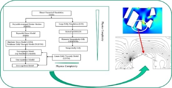
Indoor environments are influenced by indoor airflow rate, temperature, humidity, and indoor air pollutant concentrations, that are strictly governed by transport equations consisting of the continuity equation of mass conservation, three momentum conservation, and energy conservation equations, the Navier–Stokes equations [8,9]. These are driven by the combined forces of the external wind, interior mechanical fans, and thermal buoyancy, and are further complicated by the turbulent characteristics of airflows. Figure 1 shows an example of just such a ventilated room where separation, reattachment, transition to turbulence, and recirculation or vortex formation are present. Since the airflow in a building system is generally turbulent, random, multiscale, and complex in nature, the governing Navier–Stokes equations do not permit analytical solutions.
Hence, the typical practice is to solve the Navier–Stokes equations numerically to capture the physical features of the problem at hand. Computational Fluid Dynamics (CFD) has been employed widely especially for this purpose. An example of CFD calculations for determining the pressure distribution around a house is shown in Figure 2, where the left inlet velocity is set at 3 m/s.
The proper selection of a turbulence modelling method and grid generation is of great importance to the simulation accuracy of the turbulent airflow. Very often the turbulence models are inconsistent with the phenomenon in question since the characteristics of airflow distribution are often difficult to identify or too complex for CFD because the phenomenon is beyond what is computationally possible. These problems are not completely understood or resolved in building energy applications [10,11].
2. Fundamentals of Fluid Dynamics Models
2.1. Model Equations
The basic governing equations of fluid flow are
- Conservation of mass
- Conservation of momentum (Navier–Stokes equation)
- Conservation of energy
For many building energy studies, a Newtonian fluid with uniform viscosity is assumed, and the constitutive equation for is expressed as
where μ is the dynamic viscosity coefficient, I is the identity tensor, and the kinematic viscosity coefficient υ = µ/ρ.
In particular, for incompressible fluid without external force, the equations can be simplified. To close out the equation system, constitutive equations of thermodynamic properties are needed to relate the state variables. For buoyancy-driven flow that dominates building ventilation, the ideal gas equation or the Boussinesq approximation is generally used to relate densities to temperatures.
2.2. An Overview of Fluid Dynamics Modeling
A dimensionless analysis of the set of Navier–Stokes equations produces the Reynolds number (Re), which characterizes the flow features of the fluid. Turbulence occurs at high Reynolds numbers and is random, irregular, diffusive, dissipative, and chaotic in three dimensions and consists of eddies of many different sizes, energy levels, and structures. According to turbulence theory [12,13], eddies are formed over different length and time scales, the size of large eddies are in the same order of the mean flow, depending on the boundary conditions. The smallest eddies, characterized by the Kolmogorov scale, are universal and isotropic. Viscous dissipation of turbulence kinetic energy is associated with them. The large eddies are unstable and eventually broken up to generate smaller eddies, and therefore energy cascades from larger to smaller eddies. The turbulence theory states
where u is the characteristic velocity of large eddies, turbulent kinetic energy, ε the dissipation rate, and τ the time scale of large eddies. From Equation (5), the turbulent length and time scales of large eddies are
where l is the length scale of large eddies. At the Kolmogorov scale,
The major challenge in modelling turbulence comes from the wide range of time and length scales in which turbulent mixing occurs and energy is transferred. The evolving eddy structure of the turbulence is still not fully understood.
Until now three basic models can be generalized: (1) the Direct Numerical Simulation (DNS) model which resolves all the scales of the turbulent flows without any models or approximations; (2) the Reynolds-averaged Navier–Strokes (RANS) model which resolves the mean flow and average out the turbulent fluctuations; and (3) the Large Eddy Simulation (LES) that lies between the models of DNS and RANS regarding the resolved scales. Comparison of the computational costs is shown in Table 1, where the ratio of the largest to smallest length scales on the order of Re3/4 is used based on the Kolmogorov theory [12,13,14].
Table 1 shows that DNS has the highest level of physics modelling and cost while RANS has the least. Consider a typical indoor airflow in a small mechanically ventilated office with Re = 5000. DNS requires a grid on the order of 1010 and minute calculation of 106 [15]. In much practical indoor airflow where typically Re = 104–105, the required grid sizes of DNS and LES are in the range of 1012–108, exceeding the capacity of most contemporary computers.
The relatively low computational cost of RANS makes it the most commonly used turbulence model in building energy research. However, RANS is not capable of accurately predicting certain complex flows, for example, separated flows. Thus, even with today’s supercomputers, the single largest challenge is the balance between reliable accuracy and affordability of the CFD model for turbulent flow, especially for high Reynolds number simulations. The following is an overall review of the popular mainstream turbulence models including a brief description of DNS models.
3. Direct Numerical Simulation (DNS) and Turbulence Models
3.1. DNS Models
DNS models are the most accurate CFD method with high resolution and computational cost. In terms of practical applications where Reynolds numbers are generally on the order of 106–108 for the flows around buildings and on the order of 105 inside buildings, DNS is not practical. Moreover, higher orders of accuracy are needed in order to secure higher-order closures. High-order methods are still an open question in many aspects, regarding, for example, mesh generation and numerical stability. The majority of DNS models, therefore, have been limited to theoretical studies of near-wall turbulence models for natural and forced convection flow in building spaces [16,17,18]. To understand infectious COVID-19’s dynamic transmission mechanisms under cough and sneeze flows [19], the DNS model was applied. The cumulus cloud flow DNS model including phase change thermodynamics and the dynamics of small water droplets was combined with generated data from these flows. DNS models are not feasible, generally. This leads to the wide application of the turbulence models based on RANS and LES approaches.
3.2. Turbulence Models
The most widely used current method for modelling turbulent flows is the RANS approach. RANS decomposes the flow field, velocities, and pressures into the mean and fluctuating parts as:
where the mean values are averaged over time and . For an incompressible Newtonian flow, the averaging procedure gives
and the Reynolds stress
In contrast to the RANS method, the LES approach separates small eddies and large eddies based on a spatial filter. The flow field is decomposed as filtered and residual subgrid-scale (SGS) parts as:
where the filtered component is
for the whole volume V of the flow and the filter function F satisfies . The commonly used filter functions are top hat (or box), Gaussian, and spectral cut-off functions [20], for example, the top hat filter
where Δ is the filter width.
The filtered Navier–Stokes equations become
and the subgrid-scale (SGS) Reynolds stress
τijLES plays a similar role in LES as τijRANS in RANS.
3.3. Near-Wall Turbulence Models
Near-wall boundary modelling is especially important in building research from a physical point of view because walls are a major component of a building and they determine flow separation, transition, and reattachment around and inside the building. Additionally, most temperature changes occur across such a boundary. Numerous experiments have shown that the velocity profile at the near-wall region can be basically categorized into three boundary layers: the viscous sublayer, buffer layer, and the fully turbulent layer. The turbulence develops and grows from the viscous sublayer (laminar) to the fully turbulent layer (fully turbulent) with laminar-turbulent transition. This corresponds to the velocity and temperature increase from the no-slip condition and wall temperature to a maximum velocity and the temperature in the main stream of the flow.
For modelling the near-wall region, the most essential requirement is the accurate determination of the near-wall flow gradients of the flow profiles. However, turbulent flow conditions with very steep gradients near the walls result in very thin boundary layers and the inhomogeneous and anisotropic flows in the thin boundary layers are difficult to resolve and capture. In the viscous sublayer, the viscosity dominates and the convection can be neglected while in the fully turbulent layer, the opposite effects determine the flow. The buffer layer presents the transitional layer while the only dominant variable is the normal distance from the wall. This phenomenon near the wall should be correctly reproduced by turbulent models and special treatments are generally needed to ensure consistency with the boundary layer flows [21]. The success of the turbulent models is mostly judged by the performance of the models in the near-wall regions. The near-wall behavior of RANS and LES and the treatments will be briefly reviewed in the following relating sections for the relevant models.
4. Reynolds-Averaged Navier–Stokes (RANS) Models
RANS models can be classified into two major groups depending on how the Reynolds stresses τijRANS (see Equation (10)) are formulated. The most common approach to modelling Reynolds stresses is the eddy viscosity model (EVM) in which the Reynolds stress is expressed according to the eddy viscosity hypothesis model EVM to link the mean flow with the turbulence feature. Another approach is provided by the Reynolds stress models (RSM).
4.1. Eddy Viscosity Models (EVMs)
The EVM models can be further divided into linear (LEVM) and nonlinear (NLEVM) models [21]. LEVMs are further classified as zero-, one-, and two-equations, related to the number of transport equations and the approaches to calculating velocity and length scales (see Equation (5)).
The zero-equation, or the mixing length, model was originally introduced by Prandtl [22]. In this model, the transport equation is not solved and the eddy viscosity represents a global value for the mean velocity and length scales [23]. The one-equation model solves one transport equation for velocity scale and the length scale is determined algebraically. The standard Spalart–Allmaras (S-A) model [24] is the most popular one-equation turbulence model because of its simplicity and acceptable accuracy. Both zero-equation and one-equation are cost-effective; however, neither is used as a general turbulence model.
Two-equation models are sometimes referred to as complete models because two quantities are employed to characterize both velocity and length scales and solve them independently. Most often the velocity scale is k1/2 but the length scale l varies. This allows turbulence production and dissipation to have localized rates and leads to more accurate models. Therefore, two-equation models offer a good compromise between computational effort and accuracy. The standard k-ε turbulence model [21] is the most commonly used turbulence model and it is still by far the most popular model. It also has well-known drawbacks that produce inaccurate prediction for some complex flows involving severe pressure gradient, separation and recirculation.
4.2. Reynolds Stress Models (RSMs)
Besides LEVM, nonlinear eddy viscosity models (NLEVM) have also been proposed to improve LEVM. NLEVMs serve the intermediate level models between LEVMs and RSMs. Originating from [29] and referred to as a second order or moment closure, RSMs present another large class of turbulence models. In the RSMs, without the isotropic eddy viscosity hypothesis, the Reynolds stresses are derived in the exact form that accounts for anisotropic Reynolds stress fields. The computational cost is high.
A simplified alternative of RSM is the algebraic stress models (ASM) proposed by Rodi [30]. The basic idea is to approximate the differential Reynolds stress terms in such a way that the modelled equations become algebraic. Since the transport equations for k and ε have to be solved in ASM models, ASMs are sometimes referred to as NLEVMs. RSMs are used within a sufficiently small region in studying significant anisotropic turbulence in building energy research.
4.3. Near-Wall Treatment
In the near-wall regions where Reynolds numbers are low and viscosities dominate, neither the kε nor the k-ω formulations can produce the near wall physics correctly. Near-wall treatment is needed and remains difficult physically [31]. There are basically two approaches: wall function and near-wall modelling strategies. The first uses empirical formulae as algebraic wall functions to bridge the gap of the inner and outer regions. Near-wall modelling strategies solve governing equations for the viscous sublayer up to the wall without using the wall functions. Simple mixing-length zero-equation model is often used for the sublayer.
Low-Reynolds-Number (LRN) models [32] have been used for heat transfer problems where thermal transfer at the walls is important for the whole domain’s thermal field. However, for some special complex flows, for example, the buoyancy-driven types, the models are not accurate enough [33]. In the authors’ experience, LRN models aim specifically at an improved modelling of near-wall performance. They may not be efficient for low-Reynolds-number flows that are not in the near-wall regions. A two-layer model created by unifying two different turbulence models is often used: one for high-Reynolds-number flows in the outer region and another one for LRN model in the near-wall region (two-layer k-ε model in [34]). Various enhanced wall treatment and hybrid strategies have also been proposed for higher accuracies, see [35,36] in building applications.
5. Large Eddy Simulation (LES) Models
5.1. An Overview
The rationale behind LES is based on the fact that energy tends to travel from large turbulence scales to smaller ones, but not in the reverse [37]. Therefore, LES resolves the large turbulence scales containing most of the turbulent kinetic energy while the effects of small energy-dissipating scales are modelled using SGS models which could be much simpler than the RANS model equations. LES provides a more detailed analysis of the turbulence structure compared to RANS.
The classical Smagorinsky–Lilly model [38,39] is one of the most popular SGS models due to its simplicity and numerical stability; however, it has several drawbacks, mainly related to the choice of the model coefficient. The model is not accurate enough for transitional flows. The dynamic Smagorinsky–Lilly (LES-DYN) model [40] applies a dynamic modelling concept that presents a major step in SGS modelling. The main idea is to filter the resolved scales using a larger filter to relate SGS stresses at the two levels to calculate the varying coefficients of the Smagorinsky model.
The variational multiscale (VMS) methods extend classical filtering approach in LES models in such way that spatial filtering is replaced by the variational projection [41]. The VMS method decomposes the flow field into three scales: large, resolved small, and unresolved (small) scales. The unresolved scales are generally assumed not directly influence the large scalesbut indirectly, influence the resolved small scales only. VMS has been found to perform better than the Smagorinsky and dynamic LES-DYN models [42].
5.2. Near-Wall Treatment
Although LES is generally expected to be more accurate than RANS, it faces a serious challenge for high-Reynolds wall-bounded flow where the dissipation takes place in smaller eddies. More stringent resolution requirements are then needed to resolve the dynamically important and small eddies in the near-wall region with the cost comparable to a DNS. LES models are currently restricted to relatively low-Reynolds-number flows. Generally, it is only recommended to model flows where wall boundary layers are generally irrelevant in practical calculations; otherwise, special near-wall treatment is needed.
Two common approaches have been proposed: wall stress models and hybrid RANS/LES techniques. The hybrid RANS/LES method has proven successful in the past in paving the way to improve turbulence modelling research. In building energy applications, however, hybrid RANS/LES models have not been efficiently performed for indoor airflows [43] with very limited applications. Despite the gaps, hybrid RANS/LES modelling has shown promising results and is a very active research topic. Figure 3 summarizes the hierarchy of the described turbulence models.
6. Implementation and Software
Simulation involves CFD software implementation of turbulence models and the software generally contains pre-processing, solving, and post-processing modules. The core of the CFD software is the solver that includes mesh generation for the geometry of the defined problem, discretization of the model equations, the solution of the resultant algebraic equations, and the handling of nonlinearity and inter-equation coupling. Commonly used discretization and solution algorithms include finite difference, finite element, and finite volume approaches combined with explicit and implicit integration over time [44]. For RANS, it is important to ensure correct and well-defined turbulence kinetic energy boundary conditions. For LES, high-accuracy discretization should be adopted to minimize the numerical dissipation. Some advanced techniques involve spectral elements, higher-order, and adaptive numerical approximations in discretization and solution methods are described in [45].
Many commercial CFD software packages are now available. Some of the most commonly used codes used in energy and building research are shown in Table 2.
Although most of these CFD software packages provide robust and higher resolution simulations, geometry, mesh generation, and grid quality are still a challenge in using these software packages.
7. Applications
This section looks at some of the areas in which the reviewed CFD models have been applied to help in understanding the advantages, drawbacks, and application ranges of the turbulence models. Two research directions can be categorized. The first are engineering efforts to adjust models for various flow applications. A second category is composed of research that mainly compares the model performance. Both may involve the methodological and practical aspects. As RANS models have been much more widely used, we draw an attention to RANS models. It is worth mentioning that application of CFD in building energy research is wide and for many purposes, and there are no clear-cut rules for separating them in many applications.
7.1. RANS Models
RANS models are the basis for most building energy simulations. There are several popular application areas in which RANS models have been applied: ventilation, urban, and pedestrian thermal and wind environments, indoor airflow and transport, dispersion, deposition of pollutants. The impact of ventilation on airborne transmission of COVID-19 virus in buildings constitutes the recent research topic. Among RANS models, the standard k-ε, RNG k-ε, standard k-ω, and SST k-ω models score the highest.
As ventilation plays a central role in building energy consumption and indoor air quality, it constitutes a major part of CFD airflow applications, accounting for 70% of the ventilation models published in the main international journals already in 2009 [11]. This number is much higher now when including indoors and ventilation mitigation strategies for preventing COVID-19 pandemic. Among the most important and popular applications is the design and control of natural ventilation systems.
The zero-equation model was initiated to simulate various ventilation based on natural, forced, mixed convection, and displacement with three-dimensional air velocity, temperature, and contaminant concentrations in a room. The simulation results agreed reasonably with both the measured data and the standard k-ε model [11]. The zero-equation model was initiated [46] to study mixed air flow ventilation and moisture transport across a large horizontal opening. The model was compared with two-story testing hut in full scale. The zero-equation model has been also applied in many other areas of building simulations.
The standard k-ε and the standard k-ω models have had much wider use in studying the natural ventilation as a low-energy environmental solution. The research problems arise from a range of topics such as the performance of wing walls for the integration of environmental, energy, and ecological issues into building design [47], indoor air flow induced by wind in a building adjacent to a vertical wall for the aim of reducing the building cooling load [48], the steady-state convection in a double-paned window for energy efficient window rating and design [49], a greenhouse’s indoor air environment with a transparent bubble envelope and the thermal energy efficiency of the envelop [50], the unsteady-state flow in a naturally ventilated space with source of heat in the central place [51], the natural ventilation under different wind incidences in a climatic livestock building with varied areas of the inlet opening [52], and ventilation cooling and airflow and heat transfer characteristics in vertical cavities with variations in different physical parameters (dimensions such as height and widths, heat fluxes, distributions of wall heat, etc.) [53]. A series of small-scale laboratory experiments were conducted and compared with the measurements in [51]. At the beginning of the room stratification, the simulations were accurate. However, for longer times, the results diverged. Applications in personalized ventilation were reviewed in [54].
Another active application area is the application of RANS for the assessment of impact of ventilation rates on indoor airflow and energy use. Here, the main interest is the simulation of the indoor airflow patterns, distribution, and velocity as well as the temperature distribution in different configurations of buildings, such as different locations of the air conditioner blower [55], and enclosed-arcade markets [56]. RNG k-ε models were employed to study a historical building with an ancient natural ventilation system [57], energy use, comfort, and condensation for both single and double glazed facade buildings [58], and optimization of indoor environment [59]. Double glazed facade with natural ventilation demonstrated a minimized energy consumption as well as enhancing the thermal comfort in [58]. Ramponi and Blocken [60] applied the SST k-ω model to investigate wind-induced cross ventilation of buildings in four configurations compared with wind tunnel measurements. The measurements showed good agreement with the model. Hussain and Oosthuizen [61] also applied the SST k-ω model to investigate three-storey atrium building and its buoyancy-driven natural ventilation induced by solar radiation and heat sources. These models, the SST k-ω model for example, have been applied in building hydronic heating radiant ceilings and walls for optimizing both energy consumption and comfort for [62].
Outdoor airflow simulation is an important topic, since wind is the driving force in cross ventilation. Due to computer capacity limitations, much outdoor airflow simulation has been simulated separately to provide boundary information for indoor airflow and ventilation models. Research objectives were to study convective heat transfer coefficients at the windward facade of a low-rise cubic building [63], wind-induced ventilation efficiency in void spaces in built-up urban areas [64], a hybrid ventilation system combing both natural and mechanical ventilation [65], atmosphere boundary layer flow around buildings [66], wind power application in buildings [67], optimization of the device performance in terms of internal velocity and pressure for different microclimates under varied external angles of windvent louvres [68], the urban wind flow and indoor natural ventilation [69], and the induced flow patterns around and inside a building [70]. In order to improve the wind comforting environment in complex urban areas, the standard k-ε model was applied in [71] in a real urban area in the city. About 920 different configurations of different heights and plan area densities were considered and evaluated. More research can be found in [72].
Exceptionally extensive research has been conducted recently on COVID-19 virus transmission mechanisms and the current indoor air ventilation measures, standards, and mitigation strategies because the coronavirus is continuing to pose weighty challenges for people around the world. A comprehensive review of various CFD models, finite element methods, and in vitro experiments were conducted by Mutuku et al. [73] on human airways of the airflow and aerosol motion and the possible pathways of airborne transmission of the COVID-19 virus. Human airways in different medical conditions (healthy and unhealthy) were considered. Table 3 shows some results.
Both [73,84] investigated energy issues also. In order to reduce indoor bacterial concentration, the effects of the use of upper indoor ultraviolet germicidal irradiation (UVGI) systems and the increase of outdoor air volume were compared in [73]. Results showed that UVGI systems were a more economical means. The rated power of UVGI systems is very small that can be neglected in terms of HVAC systems’ energy consumption, with the absolute increase of the energy consumption being only 0.45%. The impact of increasing outdoor ventilations on space heating demand was investigated in [84]. The results showed that energy consumption increased by only 51.6% using heat recovery devices, corresponding to the outdoor ventilation increase by three times. The conclusion is that significantly improved energy efficiency of the HVAC system can be obtained by using heat recovery systems. It can efficiently mitigate the increased energy consumption of HVAC systems during the coronavirus epidemic.
7.2. Comparison of RANS Models
Due to a variety of turbulence modelling options among RANS, it is often not clear which turbulence model to apply. Evaluation and testing of predictions by different types of RANS models has been object of much study, with efforts made at comparing, validating, and improving the models in order to obtain a clear picture of the capabilities of these models. Table 4 summarizes the model performances based on our exhaustive review. Only representative articles are cited in the table. To understand these models, brief application scenarios are also provided.
Our literature review and Table 4 show that RANS models are the most economical and widely used models, and they generally are able to provide the level of accuracy required. Paper [104] examined the most commonly used turbulence models including standard k-ε, two-equation k-ε, RNG k-ε, SST k-ω, RSM, and LES for their prediction capabilities on natural convection with respect to modelling strategies, such as simulation of the approach boundary layer, consideration of two-dimensional and three-dimensional simulations and the use of domain decomposition. The trajectories of external and internal flows, the flow rates of cross ventilation and internal pressure were modeled. The internal flows and the cross-ventilation flow rates were found to be insensitive to the models. In general, two-equation models are adequate in most cases. The RNG k-ε, the SST k-ω, and the standard k-ε have the best overall accuracies among two-equation models, even whilst each model has good accuracy and is suitable for certain types of fluid flow. Among them, the RNG k-ε model performs better than the standard k-ε model and the SST k-ω model has the best overall performance.
In certain cases, however, some models are not suitable ones. A case study using different RANS models was studied in [103]. The standard and realizable k-ε models had better accuracy, compared with the standard k-ω and SST k-ω model. Two-equation models suffer from several limitations especially for transition and flow separation flows. Experimental evidence has shown that indoor airflows are transitional when the Reynolds number for the supply air is between 2000 and 3500. Airflow separation occurs over building sharp edges. The same phenomena happen for the outdoor environment around buildings. Paper [36] presented a focus on various applications and found that RANS is not accurate enough for calculations of the transient separation and recirculation flow at windward edges, and of the Von Karman vortex street. To determine the most suitable turbulence model for naturally ventilated livestock buildings, [104] compared four RANS models, including standard k-ε, RNG k-ε, and the SST k-ω with measurements. They obtained surprising results: neither could adequately predict near-wall boundary layer flow, as similar results were obtained by using the standard k-ε and the RNG k-ε models. Away from the boundary layer, the RNG k-ε model did not outperform the standard k-ε. Additionally, the prediction of the SST k-ω was unsatisfactory. In complex indoor and outdoor air flow environments, turbulent flows may involve transition, separation, recirculation, and buoyancy; models perform differently for different cases; and, hence, mixed results have been reported. Paper [105] recommended the standard k-ε model with enhanced near-wall treatment based on comparative studies on commercial CFD software, e.g., FLUENT, STAR-CD, and ANSYS CFX.
7.3. LES Models
LES models usually come for predicting complex flows when RANS methods are inadequate. Jiang and Chen [106] studied single-sided natural ventilation in buildings, where RANS were inaccurate. Smagorinsky and the LES-DYN models were applied and found to have sufficiently good accuracy for fully developed high Reynolds number turbulence flow. However, if the flow presented mixed features with both turbulent and laminar properties, the Smagorinsky model couldn’t reach accurate results. The same conclusion was obtained for the flow with a significant wall effect. Thermal dispersion gas flow simulation was carried out in [107] by employing both the standard k-ε model and LES model for unsteady state turbulent flow behind a high-rise building. Results show that the standard k-ε model overestimated the dispersion and that the LES was accurate. For building outdoor environments, [108] adopted a LES-DYN to study wind flows of a station building with a complex roof. The modeling results had a good agreement with the wind tunnel test data. Liu et al. [109] studied convective heat transfer coefficients at the external windward, leeward, lateral, and top surfaces of buildings. The realizable k-ε, the SST k-ω model, and the Smagorinsky model were compared with experimental data. Although all the models were validated with the experimental data, RANS models overestimated convective heat transfer coefficients generally.
To improve the urban canopy parameterizations in mesoscale modeling in [110], the LES model was adopted and the simulation results were validated using the wind tunnel experiment. Available LES and DNS data were also compared with the simulation results. LES mode was found to outperform RANS [110]. Using LES models, a square prism in a uniform flow was investigated in terms of its aerodynamic characteristics under various angles of attack [111]. The results agreed favorably with experiments. For the same air change rate, different natural ventilation patterns, airflow behaviors, and the transport of particulate matter were modelled via LES in [112]. An empirical equation was constructed to predict both the mean ventilation rate and fluctuating ventilation rate. LES simulation, with an experiment, was used to validate the developed empirical formula [113]. Using Smagorinsky and LES-DYN models, [114] studied airflows around different configurations of blocks for pedestrian-level wind. Simulation results were analyzed and the relationship between the building geometry and the pedestrian zone wind speed was derived theoretically. Paper [115] explored surface pressure, local wall-normal forces, and cross-wind velocity on tall buildings through LES. Paper [116] applied LES to simulate turbulent buoyancy-driven flows for building-integrated photovoltaic systems mounted on building façades and roofs.
Recently, wind farms as a renewable energy are becoming popular and attracting research on their wind flow characteristics. Turbulent wind flow features for wind turbines in relation to energy production have been widely investigated. Flows of the wind farms were modeled using the LES model by Wu et al. [117]. They investigated the wind turbine behavior under different farm layouts and the resulting flow structures. Stevens et al. [118] applied LES models for finite length wind farms targeting the effects of atmospheric and wake turbulence. Yang et al. [119] investigated offshore wind farm energy using LES with both wind-seas and swells under moderate wind speeds. Further, various sensitivity studies of LES to model parameters have also been performed to provide practice guidelines [120]. Wang and Chen [121] investigated eight turbulence models for transient airflow in an enclosed environment and compared the results with experimental data. Transitional flow of jet, separations, and thermal plumes was considered. LES was found to be the most accurate model.
For LES validation and comparison with RANS models, Vita et al. [122] simulated the flow pattens around high-rise buildings based on the turbulent inflow variations. It was found that RANS models are accurate only for some situations. LES models are generally reliable. A similar setting of a high-rise building with balconies was investigated by Zheng et al. [123] with similar comparison results obtained for the RANS and LES models. RANS are conditionally accurate. The same authors [124] validated LES by wind tunnel experiments in studying other setting variations for high-rise buildings.
These results reveal the applicability of LES models. However, LES models are computationally intensive and are not always cost-effective. Vita et al. [125] investigated the flow pattens on the roof of tall buildings based on the turbulent inflow variations and the geometric model. They found that LES accuracy is only marginally affected by factors like inflow mean wind speed and other turbulence factors. Taghinia et al. [126] studied the impact of airflow on the occupants to determine the ventilation method for energy and indoor air quality. The LES model was improved in [126]. Figure 4 shows the simulation.
Recently, LES models have been also applied in the modeling of indoor airborne transmission for studying the COVID-19 pandemic. Vuorinen et al. [127] performed LES to model the aerosol transport over long distances in order to model the aerosol and droplet dispersion in relation to aerosol transmission of SARS-CoV-2. They claimed LES to be the most accurate of CFD models. Similarly, using the LES model, indoor airborne transmission in relation to the variations of mouth opening characteristics was studied in [128]. A correlation was established between the direct reaching area and the intensities of the coughs. For a restaurant setting, the indoor airflow and the associated aerosol were investigated in [129]. There have been lots of reports by the media on the contamination of asymptomatic COVID-19 cases in similar settings. The LES model was adopted to simulate the flow structures on aerosols.
8. Discussion and Conclusions
This paper has provided an in-depth review of fluid dynamics models for building energy research, with an extensive account of the theoretical interpretations, assumptions, critiques, modelling robustness and purposes, application ranges, and behavioral aspects of the most influential models encountered in the literature. A comparative evaluation of the effectiveness of the models from the most recent and relevant publications has been presented. There are reviews of application-oriented models in the literature (e.g., [54,72,130,131]), but none of these consider the fluid dynamics models from such a broad perspective of methodologies. In this respect, our review fills that void.
As the most accurate turbulence model, DNS resolves all scales of turbulence, has the highest predictive accuracy, and can be used as a benchmark reference to gain a fundamental understanding of the physical process which is not possible to gain by using other turbulence models. However, DNS is too computationally expensive for current computers and, therefore, its application remains extremely limited to low Reynolds number flows mainly. RANS, on the other hand, models all scales of turbulence and represents the most popular models in building energy applications. For certain complex flows, LES models can capture turbulent variations and dynamics more accurately than RANS models. However, strongly anisotropic flows at near-wall with high Reynolds numbers are a major challenge for both RANS and LES models. Hybrid modelling has generated much interest among researchers as a promising solution for effectively solving these challenges by combining the advantages of both RANS and LES. However, applications of the hybrids appeared to be extremely limited in building energy research. From an implementation perspective, the complexity of CFD software operation, complicated meshing techniques, and long calculation time present challenges. Reliable meshing for complex geometries will be the key to the success of CFD models.
All of the reviewed models have advantages and disadvantages with respect to their modelling accuracy, details, and application scope. The choice depends on the complexity and level of details of the analysis and the computational efficiency that needs to be achieved for the practical problems. There are several issues that need particular attention. First, the choice of appropriate modelling methods and the model is of crucial importance because state-of-the-art building simulation modelling relies on physical assumptions and empiricism. In many applications, it is recommended to combine and compare different turbulence models. Second, numerical techniques play an important role. For example, the accuracy of RANS or LES relies greatly on the employed numerical methods and mesh sizes. The most significant numerical issue associated with simulations is the grid dependency, as mentioned previously. This dependency should be minimized as much as possible.
Finally, an important issue is the ability to model the evolving smart and complex building systems that contain a large number of components with unknown multiple physical mechanisms. Multiscale modelling techniques are uniquely positioned to model complex multi-physics phenomena. Multiscale models have been adopted in some areas of building research [132,133], although they are still in the early stages of development. Furthermore, various data-driven models have been adopted to cope with the challenges of uncertainty. A crucial limitation of the pure data-driven approach is its generalization capability. Large quantities of data are needed and the models are often difficult to interpret. Data-driven models that can support physical interpretation and inference of building systems are more desirable. A contemporary trend is to couple fluid dynamics models and data-driven models. This type of model is more efficient in modelling complex buildings that involve many uncertainties and randomness with physical mechanisms that are too complex to be understood. Such hybrid modelling is the area undergoing the most rapid development.
Author Contributions
Conceptualization, X.L. and Z.D.; methodology, X.L., T.L., T.Y.; investigation, H.S. and P.D.; writing—original draft preparation, X.L. and T.L.; writing—review and editing, H.C.; supervision, X.L., Z.D., and H.C.; funding acquisition, X.L. and Z.D. All authors have read and agreed to the published version of the manuscript.
Funding
This research was supported by the Academy of Finland (STARCLUB, Grant No. 324023 and CLEANSCHOOL, Grant No. 330150) and the National Natural Science Foundation of China (Grant No. 41972324).
Conflicts of Interest
The authors declare no conflict of interest.
Nomenclature
| E | total energy |
| F | filter function |
| gravitation vector | |
| h | enthalpy |
| I | identity tensor |
| i, j | indices (coordinate system or zones) |
| k | turbulent kinetic energy per unit mass |
| l | length scale of large eddies |
| P | pressure |
| flux vector | |
| heat source | |
| t | time |
| T | temperature |
| u | velocity |
| velocity vector | |
| filtered velocity | |
| V | volume |
| x, y, z | space coordinate |
| Greek | |
| Δ | filter width |
| ԑ | dissipation rate per unit mass |
| λ | thermal conductivity |
| μ | dynamic viscosity |
| υ | kinematic viscosity |
| ρ | density |
| τ | time scale |
| , | Reynolds stress tensor (RANS, LES) |
| viscous stress tensor | |
| ω | specific dissipation |
| Operators | |
| substantial derivative | |
| , | time averaged u, corresponding fluctuation of u |
| , | spatially filtered u, corresponding fluctuation of u |
| ∇ | gradient |
| Superscripts/subscripts | |
| η | Kolmogorov scale |
| ω | related to k-ω model |
| Glossary of acronyms | |
| ASM | Algebraic Reynolds stress |
| CFD | Computational fluid dynamics |
| DNS | Direct numerical simulation |
| EVM | Eddy viscosity model |
| HVAC | Heating, ventilation, and air conditioning |
| LES | Large eddy simulation |
| LES-DYN | Dynamic Smagorinsky–Lilly |
| LEVM | Linear eddy viscosity model |
| LRN | Low-Reynolds-number |
| NLEVM | Nonlinear eddy viscosity model |
| RANS | Reynolds averaged Navier–Stokes |
| Re | Reynolds number |
| RSM | Reynolds stress model |
| RNG | Re-Normalisation Group |
| S-A | Spalart-Allmaras |
| SGS | Subgrid-scale |
| SST | Shear stress transport |
| UVGI | ultraviolet germicidal irradiation |
| VMS | Variational multiscale |
References
- European Commission. Eurostat Energy, Transport and Environment Indicators; European Commission: Brussels, Belgium, 2014; Available online: https://cn.bing.com/search?q=Energy%2C%20transport%20and%20environment%20indicators%20%E2%80%94%202014&qs=n&form=QBRE&sp=-1&pq=energy%2C%20transport%20and%20environment%20indicators%20%E2%80%94%20201&sc=0-50&sk=&cvid=6AB91FAB166149C4BDC08BF3A8137779# (accessed on 20 August 2021).
- EIA. Annual Energy Review 2010; U.S. Energy Information Administration—U.S. Dept. of Energy, Office of Energy Statistics: Washington, DC, USA, 2011; Available online: https://cn.bing.com/search?q=Annual%20Energy%20Review%202010%3B%20U.S.%20Energy%20Information%20Administration&qs=n&form=QBRE&sp=-1&pq=annual%20energy%20review%202010%3B%20u.s.%20energy%20information%20administration&sc=0-65&sk=&cvid=F6ECBB6599204C8BB69F1CE059A7057A# (accessed on 20 August 2021).
- Directive 2010/31/EU, Energy Performance of Buildings Directive 2010; The European Parliament and of the Council: Washington, DC, USA, 2010.
- Directive 2012/27/EU, On Energy Efficiency, Amending Directives 2009/125/EC and 2010/30/EU and Repealing Directives 2004/8/EC and 2006/32/EC; The European Parliament and of the Council: Washington, DC, USA, 2012.
- European Union. Commission Staff Working Document; European Union: Brussels, Belgium, 2016. [Google Scholar]
- Huynh, A.; Barkokebas, R.D.; Al-Hussein, M.; Cruz-Noguez, C.; Chen, Y. Energy-Efficiency Requirements for Residential Building Envelopes in Cold-Climate Regions. Atmosphere 2021, 12, 405. [Google Scholar] [CrossRef]
- CDC. Available online: https://www.cdc.gov/mmwr/volumes/70/wr/mm7031e2.htm (accessed on 29 July 2021).
- Doering, C.; Gibbon, J. Applied Analysis of the Navier-Stokes Equations; Cambridge University Press: Cambridge, UK, 1995. [Google Scholar]
- Sohr, H. The Navier- Stokes Equations: An Elementary Functional Analytic Approach; Birkhäuser Verlag: Basel, Switzerland, 2001. [Google Scholar]
- Hussain, S.; Oosthuizen, P.; Kalendar, A. Evaluation of various turbulence models for the prediction of the airflow and temperature distributions in atria. Energy Build. 2012, 48, 18–28. [Google Scholar] [CrossRef]
- Chen, Q. Ventilation performance prediction for buildings: A method overview and recent applications. Build. Environ. 2009, 44, 848–858. [Google Scholar] [CrossRef]
- Kolmogorov, A.N.; Tihomirov, V.M. E-entropy and e-capacity of sets in functional spaces. Am. Math. Soc. Transl. 1959, 2, 277–364. [Google Scholar]
- Pope, S.B. Turbulent Flows; Cambridge University Press: Cambridge, UK, 2000. [Google Scholar]
- Chapman, D.R. Computational Aerodynamics Development and Outlook. AIAA J. 1979, 17, 1293–1313. [Google Scholar] [CrossRef]
- Wang, M.; Chen, Q. On a Hybrid RANS/LES Approach for Indoor Airflow Modeling (RP-1271). HVAC&R Res. 2010, 16, 731–747. [Google Scholar] [CrossRef]
- George, W.K.; Capp, S.P. A theory for natural convection turbulent boundary layers next to heated vertical surfaces. Int. J. Heat Mass Transf. 1979, 22, 813–826. [Google Scholar] [CrossRef]
- Versteegh, T.A.; Nieuwstadt, F.T.M. A direct numerical simulation of natural convection between two infinite vertical diffentially heated walls: Scaling laws and wall functions. Int. J. Heat Mass Transf. 1999, 42, 3673–3693. [Google Scholar] [CrossRef]
- Trias, F.X.; Gorobets, A.; Oliva, A.; Perez-Segarra, C.-D. DNS and regularization modeling of a turbulent differentially heated cavity of aspect ratio 5. Int. J. Heat Mass Transf. 2013, 57, 171–182. [Google Scholar] [CrossRef] [Green Version]
- Diwan, S.S.; Ravichandran, S.; Govindarajan, R.; Narasimha, R. Understanding Transmission Dynamics of COVID-19-Type Infections by Direct Numerical Simulations of Cough/Sneeze Flows. Trans. Indian Natl. Acad. Eng. 2020, 5, 255–261. [Google Scholar] [CrossRef]
- Leonard, A. Energy Cascade in Large-Eddy Simulations of Turbulent Fluid Flows. Adv. Geophys. 1975, 18, 237–248. [Google Scholar] [CrossRef]
- Launder, B.E.; Spalding, D.B. The Numerical computation of turbulent flows. Comput. Methods Appl. Mech. Eng. 1974, 3, 269–289. [Google Scholar] [CrossRef]
- Prandtl, L. Bericht über Untersuchungen zur ausgebildeten Turbulenz. ZAMM 1925, 5, 136–139. [Google Scholar] [CrossRef]
- Chen, Q.; Xu, W. A zero-equation turbulence model for indoor airflow simulation. Energy Build. 1998, 28, 137–144. [Google Scholar] [CrossRef]
- Spalart, P.; Allmaras, S. A one-equation turbulence model for aerodynamic flows. AIAA J. 1992. [Google Scholar] [CrossRef]
- Yakhot, V.; Orszag, S.A. Renormalization group analysis of turbulence. I. Basic theory. J. Sci. Comput. 1986, 1, 3–51. [Google Scholar] [CrossRef]
- Shih, T.H.; Liou, W.W.; Shabbir, A.; Yang, Z.; Zhu, J. A new-eddy-viscosity model for high Reynolds number turbulent flows—Model development and validation. Comput. Fluids 1995, 24, 227–238. [Google Scholar] [CrossRef]
- Wilcox, D.C. Reassessment of the scale-determining equation for advanced turbulence models. AIAA J. 1988, 26, 1299–1310. [Google Scholar] [CrossRef]
- Menter, F.R. Two-equation eddy-viscosity turbulence models for engineering applications. AIAA J. 1994, 32, 1598–1605. [Google Scholar] [CrossRef] [Green Version]
- Launder, B.; Reece, G.J.; Rodi, W. Progress in the development of a Reynolds-stress turbulence closure. J. Fluid Mech. 1975, 68, 537–566. [Google Scholar] [CrossRef] [Green Version]
- Rodi, W. A New Algebraic Relation for Calculating the Reynolds Stresses. ZAMM 1976, 56, T219–T221. [Google Scholar] [CrossRef]
- Hanjalic, K. Achievements and limitations in modelling and computation of buoyant turbulent flows and heat transfer. In Proceedings of the 10th International Heat Transfer Conference, Brighton, UK, 14–18 August 1994. [Google Scholar]
- Patel, V.C.; Rodi, W.; Scheuerer, G. Turbulence models for near-wall and low Reynolds number flows—A review. AIAA J. 1985, 23, 1308–1319. [Google Scholar] [CrossRef]
- Zhai, Z.; Zhao, Z.; Zhang, W.; Chen, Q. Evaluation of various turbulence models in predicting airflow and turbulence in enclosed environments by CFD: Part-1: Summary of prevent turbulence models. HVAC&R Res. 2007, 13, 853–870. [Google Scholar]
- Rodi, W. Experience with two-layer models combining the k-ε model with a one-equation model near the wall. In Proceedings of the 29th Aerospace Sciences Meeting, Reno, NV, USA, 7–10 January 1991. [Google Scholar]
- Kalitzin, G.; Medic, G.; Iaccarino, G.; Durbin, P. Near-wall behavior of RANS turbulence models and implications for wall functions. J. Comput. Phys. 2005, 204, 265–291. [Google Scholar] [CrossRef]
- Blocken, B.; Stathopoulos, T.; Carmeliet, J.; Hensen, J. Application of CFD in building performance simulation for the outdoor environment: An overview. J. Build. Perform. Simul. 2011, 4, 157–184. [Google Scholar] [CrossRef]
- Davidson, P.A. Turbulence—An Introduction for Scientists and Engineers; Oxford University Press: New York, NY, USA, 2004. [Google Scholar]
- Smagorinsky, J. General circulation experiments with the primitive equations: I. The basic experiment. Mon. Weather Rev. 1963, 91, 99–165. [Google Scholar] [CrossRef]
- Lilly, D.K. On the Application of the Eddy Viscosity Concept in the Inertial Subrange of Turbulence. In NCAR Manuscript; National Center for Atmosphric Research: Boulder, CO, USA, 1966. [Google Scholar]
- Germano, M.; Piomelli, U.; Moin, P.; Cabot, W.H. A dynamic subgrid-scale eddy viscosity model. Phys. Fluids A Fluid Dyn. 1991, 3, 1760–1765. [Google Scholar] [CrossRef] [Green Version]
- Hughes, T.J.R. Multiscale phenomena: Green’s functions, the Dirichlet-to-Neumann formulation, subgrid-scale models, bubbles and the origin of stabilized methods. Comput. Methods Appl. Mech. Eng. 1995, 127, 387–401. [Google Scholar] [CrossRef]
- Holmen, J.; Oberai, A.A.; Hughes, T.J.R.; Wells, G.N. Sensitivity of the scale partition for variational multiscale large-eddy simulation of channel flow. Phys. Fluids 2004, 16, 824–827. [Google Scholar] [CrossRef]
- Girimaji, S.S.; Srinivasan, R.; Jeong, E. PANS Turbulence Model for Seamless Transition Between RANS and LES: Fixed-Point Analysis and Preliminary Results. In Proceedings of the 4th ASME-JSME Joint Fluids Engineering Conferences, Honolulu, HI, USA, 6–10 July 2003. [Google Scholar]
- Cable, M. An Evaluation of Turbulence Models for the Numerical Study of Forced and Natural Convective Flow in Atria. Master Thesis, Queen’s University, Kingston, ON, Canada, May 2009. [Google Scholar]
- Wang, Z. Adaptive High-Order Methods in Computational Fluid Dynamics, Advances in Computational Fluid Dynamics; World Scientific Publishing: Singapore, 2011. [Google Scholar]
- Vera, S.; Fazio, P.; Rao, J. Interzonal air and moisture transport through large horizontal openings in a full-scale two-story test-hut: Part 2 CFD study. Build. Environ. 2010, 45, 622–631. [Google Scholar] [CrossRef]
- Mak, C.M.; Niu, J.; Lee, C.; Chan, K. A numerical simulation of wing walls using computational fluid dynamics. Energy Build. 2007, 39, 995–1002. [Google Scholar] [CrossRef]
- Chow, W.K. Wind-induced indoor-air flow in a high-rise building adjacent to a vertical wall. Appl. Energy 2004, 77, 225–234. [Google Scholar] [CrossRef]
- Dalal, R.; Naylor, D.; Roeleveld, D. A CFD study of convection in a double glazed window with an enclosed pleated blind. Energy Build. 2009, 41, 1256–1262. [Google Scholar] [CrossRef]
- Gan, G. CFD modelling of transparent bubble cavity envelopes for energy efficient greenhouses. Build. Environ. 2009, 44, 2486–2500. [Google Scholar] [CrossRef]
- Kaye, N.; Ji, Y.; Cook, M.J. Numerical simulation of transient flow development in a naturally ventilated room. Build. Environ. 2009, 44, 889–897. [Google Scholar] [CrossRef]
- Norton, T.; Grant, J.; Fallon, R.; Sun, D.-W. Assessing the ventilation effectiveness of naturally ventilated livestock buildings under wind dominated conditions using computational fluid dynamics. Biosyst. Eng. 2009, 103, 78–99. [Google Scholar] [CrossRef]
- Gan, G. Impact of computational domain on the prediction of buoyancy-driven ventilation cooling. Build. Environ. 2010, 45, 1173–1183. [Google Scholar] [CrossRef]
- Liu, J.; Zhu, S.; Kim, M.K.; Srebric, J. A Review of CFD Analysis Methods for Personalized Ventilation (PV) in Indoor Built Environments. Sustainability 2019, 11, 4166. [Google Scholar] [CrossRef] [Green Version]
- Yongson, O.; Badruddin, I.A.; Zainal, Z.; Narayana, P.A. Airflow analysis in an air conditioning room. Build. Environ. 2007, 42, 1531–1537. [Google Scholar] [CrossRef]
- Kim, T.; Kim, K.; Kim, B.S. A wind tunnel experiment and CFD analysis on airflow performance of enclosed-arcade markets in Korea. Build. Environ. 2010, 45, 1329–1338. [Google Scholar] [CrossRef]
- Balocco, C.; Grazzini, G. Numerical simulation of ancient natural ventilation systems of historical buildings. A case study in Palermo. J. Cult. Heritage 2009, 10, 313–318. [Google Scholar] [CrossRef]
- Hien, W.N.; Liping, W.; Chandra, A.N.; Pandey, A.R.; Xiaolin, W. Effects of double glazed facade on energy consumption, thermal comfort and condensation for a typical office building in Singapore. Energy Build. 2005, 37, 563–572. [Google Scholar] [CrossRef]
- Sun, Z.; Wang, S. A CFD-based test method for control of indoor environment and space ventilation. Build. Environ. 2010, 45, 1441–1447. [Google Scholar] [CrossRef]
- Ramponi, R.; Blocken, B. CFD simulation of cross-ventilation flow for different isolated building configurations: Validation with wind tunnel measurements and analysis of physical and numerical diffusion effects. J. Wind. Eng. Ind. Aerodyn. 2012, 104-106, 408–418. [Google Scholar] [CrossRef]
- Hussain, S.; Oosthuizen, P.H. Numerical study of buoyancy-driven natural ventilation in a simple three-storey atrium building. Int. J. Sustain. Built Environ. 2012, 1, 141–157. [Google Scholar] [CrossRef] [Green Version]
- Tye-Gingras, M.; Gosselin, L. Comfort and energy consumption of hydronic heating radiant ceilings and walls based on CFD analysis. Build. Environ. 2012, 54, 1–13. [Google Scholar] [CrossRef]
- Blocken, B.; Defraeye, T.; Derome, D.; Carmeliet, J. High-resolution CFD simulations for forced convective heat transfer coefficients at the facade of a low-rise building. Build. Environ. 2009, 44, 2396–2412. [Google Scholar] [CrossRef]
- Kato, S.; Huang, H. Ventilation efficiency of void space surrounded by buildings with wind blowing over built-up urban area. J. Wind. Eng. Ind. Aerodyn. 2009, 97, 358–367. [Google Scholar] [CrossRef]
- Ji, Y.; Lomas, K.J.; Cook, M.J. Hybrid ventilation for low energy building design in south China. Build. Environ. 2009, 44, 2245–2255. [Google Scholar] [CrossRef] [Green Version]
- Yang, W.; Quan, Y.; Jin, X.; Tamura, Y.; Gu, M. Influences of equilibrium atmosphere boundary layer and turbulence parameter on wind loads of low-rise buildings. J. Wind. Eng. Ind. Aerodyn. 2008, 96, 2080–2092. [Google Scholar] [CrossRef]
- Lu, L.; Ip, K.Y. Investigation on the feasibility and enhancement methods of wind power utilization in high-rise buildings of Hong Kong. Renew. Sustain. Energy Rev. 2009, 13, 450–461. [Google Scholar] [CrossRef]
- Hughes, B.R.; Ghani, S. A numerical investigation into the effect of Windvent louvre external angle on passive stack ventilation performance. Build. Environ. 2010, 45, 1025–1036. [Google Scholar] [CrossRef]
- Van Hooff, T.; Blocken, B. Coupled urban wind flow and indoor natural ventilation modelling on a high-resolution grid: A case study for the Amsterdam ArenA stadium. Environ. Model. Softw. 2010, 25, 51–65. [Google Scholar] [CrossRef]
- Nikas, K.-S.; Nikolopoulos, N. Numerical study of a naturally cross-ventilated building. Energy Build. 2010, 42, 422–434. [Google Scholar] [CrossRef]
- Kaseb, Z.; Hafezi, M.; Tahbaz, M.; Delfani, S. A framework for pedestrian-level wind conditions improvement in urban areas: CFD simulation and optimization. Build. Environ. 2020, 184, 107191. [Google Scholar] [CrossRef]
- Toparlar, Y.; Blocken, B.; Maiheu, B.; van Heijst, G. A review on the CFD analysis of urban microclimate. Renew. Sustain. Energy Rev. 2017, 80, 1613–1640. [Google Scholar] [CrossRef]
- Mutuku, J.K.; Hou, W.-C.; Chen, W.-H. An Overview of Experiments and Numerical Simulations on Airflow and Aerosols Deposition in Human Airways and the Role of Bioaerosol Motion in COVID-19 Transmission. Aerosol Air Qual. Res. 2020, 20, 1172–1196. [Google Scholar] [CrossRef]
- Shao, X.; Li, X. COVID-19 transmission in the first presidential debate in 2020. Phys. Fluids 2020, 32, 115125. [Google Scholar] [CrossRef]
- Mathai, V.; Das, A.; Bailey, J.A.; Breuer, K. Airflows inside passenger cars and implications for airborne disease transmission. Sci. Adv. 2020, 7, eabe0166. [Google Scholar] [CrossRef]
- Abuhegazy, M.; Talaat, K.; Anderoglu, O.; Poroseva, S.V. Numerical investigation of aerosol transport in a classroom with relevance to COVID-19. Phys. Fluids 2020, 32, 103311. [Google Scholar] [CrossRef]
- Wang, J.-X.; Li, Y.-Y.; Liu, X.-D.; Cao, X. Virus transmission from urinals. Phys. Fluids 2020, 32, 081703. [Google Scholar] [CrossRef]
- Li, Y.-Y.; Wang, J.-X.; Chen, X. Can a toilet promote virus transmission? From a fluid dynamics perspective. Phys. Fluids 2020, 32, 065107. [Google Scholar] [CrossRef]
- Shao, S.; Zhou, D.; He, R.; Li, J.; Zou, S.; Mallery, K.; Kumar, S.; Yang, S.; Hong, J. Risk assessment of airborne transmission of COVID-19 by asymptomatic individuals under different practical settings. J. Aerosol Sci. 2020, 151, 105661. [Google Scholar] [CrossRef]
- Wang, J.-X.; Cao, X.; Chen, Y.-P. An air distribution optimization of hospital wards for minimizing cross-infection. J. Clean. Prod. 2020, 279, 123431. [Google Scholar] [CrossRef]
- Chillón, S.; Ugarte-Anero, A.; Aramendia, I.; Fernandez-Gamiz, U.; Zulueta, E. Numerical Modeling of the Spread of Cough Saliva Droplets in a Calm Confined Space. Mathematics 2021, 9, 574. [Google Scholar] [CrossRef]
- Wedel, J.; Steinmann, P.; Štrakl, M.; Hriberšek, M.; Ravnik, J. Can CFD establish a connection to a milder COVID-19 disease in younger people? Aerosol deposition in lungs of different age groups based on Lagrangian particle tracking in turbulent flow. Comput Mech. 2021, 67, 1–17. [Google Scholar] [CrossRef] [PubMed]
- Kanaan, K. CFD optimization of return air ratio and use of upper room UVGI in combined HVAC and heat recovery system. Case Stud. Therm. Eng. 2019, 15, 100535. [Google Scholar] [CrossRef]
- Ascione, F.; De Masi, R.F.; Mastellone, M.; Vanoli, G.P. The design of safe classrooms of educational buildings for facing contagions and transmission of diseases: A novel approach combining audits, calibrated energy models, building performance (BPS) and computational fluid dynamic (CFD) simulations. Energy Build. 2020, 230, 110533. [Google Scholar] [CrossRef]
- Chen, Q. Comparison of different k-ε models for indoor airflow computations. Numer. Heat Transf. Part B Fundam. 1995, 28, 353–369. [Google Scholar] [CrossRef]
- Chen, Q. Prediction of room air motion by Reynolds-stress models. Build. Environ. 1996, 31, 233–244. [Google Scholar] [CrossRef]
- Wright, N.; Easom, J. Comparison of several computational turbulence models with full-scale measurements of flow around a building. J. Wind Struct. 1999, 2, 305–323. [Google Scholar] [CrossRef]
- Gebremedhin, K.; Wu, B. Characterization of flow field in a ventilated space and simulation of heat exchange between cows and their environment. J. Therm. Biol. 2003, 28, 301–319. [Google Scholar] [CrossRef]
- Walsh, P.C.; Leong, W.H. Effectiveness of several turbulence models in natural convection. Int. J. Numer. Methods Heat Fluid Flow 2004, 14, 633–648. [Google Scholar] [CrossRef]
- Arun, M.; Tulapurkara, E. Computation of turbulent flow inside an enclosure with central partition. Prog. Comput. Fluid Dyn. Int. J. 2005, 5, 455. [Google Scholar] [CrossRef]
- Hu, C.; Kurabuchi, T.; Ohba, M. Numerical study of cross-ventilation using two-equation RANS turbulence models. Int. J. Vent. 2005, 4, 123–132. [Google Scholar]
- Stamou, A.; Katsiris, I. Verification of a CFD model for indoor airflow and heat transfer. Build. Environ. 2006, 41, 1171–1181. [Google Scholar] [CrossRef]
- Rohdin, P.; Moshfegh, B. Numerical predictions of indoor climate in large industrial premises. A comparison between different k-ε models supported by field measurements. Build. Environ. 2007, 42, 3872–3882. [Google Scholar] [CrossRef]
- Zhang, Z.; Wei Zhang, W.; Zhai, Z.; Chen, Q. Evaluation of various turbulence models in predicting air airflow and turbulence in enclosed environments by CFD. Part-2: Comparison with experimental data from literature. HVAC&R Res. 2007, 13, 871–886. [Google Scholar]
- Stavrakakis, G.; Koukou, M.; Vrachopoulos, M.; Markatos, N. Natural cross-ventilation in buildings: Building-scale experiments, numerical simulation and thermal comfort evaluation. Energy Build. 2008, 40, 1666–1681. [Google Scholar] [CrossRef]
- Kuznik, F.; Rusaouën, G.; Brau, J. Experimental and numerical study of a full scale ventilated enclosure: Comparison of four two equations closure turbulence models. Build. Environ. 2007, 42, 1043–1053. [Google Scholar] [CrossRef]
- Coussirat, M.; Guardo, A.; Jou, E.; Egusquiza, E.; Cuerva, E.; Alavedra, P. Performance and influence of numerical sub-models on the CFD simulation of free and forced convection in double-glazed ventilated façades. Energy Build. 2008, 40, 1781–1789. [Google Scholar] [CrossRef]
- Liu, P.-C.; Lin, H.-T.; Chou, J.-H. Evaluation of buoyancy-driven ventilation in atrium buildings using computational fluid dynamics and reduced-scale air model. Build. Environ. 2009, 44, 1970–1979. [Google Scholar] [CrossRef]
- Irtaza, H.; Beale, R.; Godley, M.; Jameel, A. Comparison of wind pressure measurements on Silsoe experimental building from full-scale observation, wind-tunnel experiments and various CFD techniques. Int. J. Eng. Sci. Technol. 2018, 5, 28–41. [Google Scholar] [CrossRef] [Green Version]
- Diarce, G.; Campos-Celador, A.; Martin-Escudero, K.; Urresti, A.; García-Romero, A.; Sala, J. A comparative study of the CFD modeling of a ventilated active façade including phase change materials. Appl. Energy 2014, 126, 307–317. [Google Scholar] [CrossRef]
- Pulat, E.; Ersan, H.A. Numerical simulation of turbulent airflow in a ventilated room: Inlet turbulence parameters and solution multiplicity. Energy Build. 2015, 93, 227–235. [Google Scholar] [CrossRef]
- Ntinas, G.K.; Shen, X.; Wang, Y.; Zhang, G. Evaluation of CFD turbulence models for simulating external airflow around varied building roof with wind tunnel experiment. Build. Simul. 2017, 11, 115–123. [Google Scholar] [CrossRef]
- Hosseinzadeh, A.; Keshmiri, A. Computational Simulation of Wind Microclimate in Complex Urban Models and Mitigation Using Trees. Buildings 2021, 11, 112. [Google Scholar] [CrossRef]
- Norton, T.; Grant, J.; Fallon, R.; Sun, D.-W. Optimising the ventilation configuration of naturally ventilated livestock buildings for improved indoor environmental homogeneity. Build. Environ. 2010, 45, 983–995. [Google Scholar] [CrossRef]
- Klinzing, W.P.; Sparrow, E.M. Evaluation of Turbulence Models for External Flows. Numer. Heat Transf. Part A Appl. 2009, 55, 205–228. [Google Scholar] [CrossRef]
- Jiang, Y.; Chen, Q. Study of natural ventilation in buildings by large eddy simulation. J. Wind. Eng. Ind. Aerodyn. 2001, 89, 1155–1178. [Google Scholar] [CrossRef] [Green Version]
- Yoshie, R.; Jiang, G.; Shirasawa, T.; Chung, J. CFD simulations of gas dispersion around high-rise building in non-isothermal boundary layer. J. Wind. Eng. Ind. Aerodyn. 2011, 99, 279–288. [Google Scholar] [CrossRef]
- Lu, C.; Li, Q.; Huang, S.; Chen, F.; Fu, X. Large eddy simulation of wind effects on a long-span complex roof structure. J. Wind. Eng. Ind. Aerodyn. 2012, 100, 1–18. [Google Scholar] [CrossRef]
- Liu, J.; Srebric, J.; Yu, N. Numerical simulation of convective heat transfer coefficients at the external surfaces of building arrays immersed in a turbulent boundary layer. Int. J. Heat Mass Transf. 2013, 61, 209–225. [Google Scholar] [CrossRef]
- Nazarian, N.; Krayenhoff, E.S.; Martilli, A. A one-dimensional model of turbulent flow through “urban” canopies (MLUCM v2.0): Updates based on large-eddy simulation. Geosci. Model Dev. 2020, 13, 937–953. [Google Scholar] [CrossRef] [Green Version]
- Oka, S.; Ishihara, T. Numerical study of aerodynamic characteristics of a square prism in a uniform flow. J. Wind. Eng. Ind. Aerodyn. 2009, 97, 548–559. [Google Scholar] [CrossRef]
- Kao, H.-M.; Chang, T.-J.; Hsieh, Y.-F.; Wang, C.-H.; Hsieh, C.-I. Comparison of airflow and particulate matter transport in multi-room buildings for different natural ventilation patterns. Energy Build. 2009, 41, 966–974. [Google Scholar] [CrossRef]
- Wang, H.; Chen, Q. A new empirical model for predicting single-sided, wind-driven natural ventilation in buildings. Energy Build. 2012, 54, 386–394. [Google Scholar] [CrossRef]
- Razak, A.A.; Hagishima, A.; Ikegaya, N.; Tanimoto, J. Analysis of airflow over building arrays for assessment of urban wind environment. Build. Environ. 2013, 59, 56–65. [Google Scholar] [CrossRef]
- Daniels, S.J.; Castro, I.P.; Xie, Z.-T. Peak loading and surface pressure fluctuations of a tall model building. J. Wind. Eng. Ind. Aerodyn. 2013, 120, 19–28. [Google Scholar] [CrossRef] [Green Version]
- Lau, G.; Sanvicente, E.; Yeoh, G.; Timchenko, V.; Fossa, M.; Ménézo, C.; Giroux-Julien, S. Modelling of natural convection in vertical and tilted photovoltaic applications. Energy Build. 2012, 55, 810–822. [Google Scholar] [CrossRef]
- Wu, Y.-T.; Porte-Agel, F. Simulation of Turbulent Flow Inside and Above Wind Farms: Model Validation and Layout Effects. Bound.-Layer Meteorol. 2013, 146, 181–205. [Google Scholar] [CrossRef] [Green Version]
- Stevens, R.J.; Graham, J.; Meneveau, C. A concurrent precursor inflow method for Large Eddy Simulations and applications to finite length wind farms. Renew. Energy 2014, 68, 46–50. [Google Scholar] [CrossRef] [Green Version]
- Yang, D.; Meneveau, C.; Shen, L. Effect of downwind swells on offshore wind energy harvesting—A large-eddy simulation study. Renew. Energy 2014, 70, 11–23. [Google Scholar] [CrossRef]
- Bazdidi-Tehrani, F.; Ghafouri, A.; Jadidi, M. Grid resolution assessment in large eddy simulation of dispersion around an isolated cubic building. J. Wind. Eng. Ind. Aerodyn. 2013, 121, 1–15. [Google Scholar] [CrossRef]
- Wang, M.; Chen, Q. Assessment of Various Turbulence Models for Transitional Flows in an Enclosed Environment. HVAC&R Res. 2009, 15, 1099–1119. [Google Scholar] [CrossRef]
- Vita, G.; Salvadori, S.; Misul, D.A.; Hemida, H. Effects of Inflow Condition on RANS and LES Predictions of the Flow around a High-Rise Building. Fluids 2020, 5, 233. [Google Scholar] [CrossRef]
- Zheng, X.; Montazeri, H.; Blocken, B. CFD simulations of wind flow and mean surface pressure for buildings with balconies: Comparison of RANS and LES. Build. Environ. 2020, 173, 106747. [Google Scholar] [CrossRef]
- Zheng, X.; Montazeri, H.; Blocken, B. CFD analysis of the impact of geometrical characteristics of building balconies on near-façade wind flow and surface pressure. Build. Environ. 2021, 200, 107904. [Google Scholar] [CrossRef]
- Vita, G.; Hashmi, S.A.; Salvadori, S.; Hemida, H.; Baniotopoulos, C. Role of Inflow Turbulence and Surrounding Buildings on Large Eddy Simulations of Urban Wind Energy. Energies 2020, 13, 5208. [Google Scholar] [CrossRef]
- Taghinia, J.H.; Rahman, M.; Lu, X. Effects of different CFD modeling approaches and simplification of shape on prediction of flow field around manikin. Energy Build. 2018, 170, 47–60. [Google Scholar] [CrossRef]
- Vuorinen, V.; Aarnio, M.; Alava, M.; Alopaeus, V.; Atanasova, N.; Auvinen, M.; Balasubramanian, N.; Bordbar, H.; Erästö, P.; Grande, R.; et al. Modelling aerosol transport and virus exposure with numerical simulations in relation to SARS-CoV-2 transmission by inhalation indoors. Saf. Sci. 2020, 130, 104866. [Google Scholar] [CrossRef]
- Pendar, M.-R.; Páscoa, J.C. Numerical modeling of the distribution of virus carrying saliva droplets during sneeze and cough. Phys. Fluids 2020, 32, 083305. [Google Scholar] [CrossRef]
- Liu, H.; He, S.; Shen, L.; Hong, J. Simulation-based study of COVID-19 outbreak associated with air-conditioning in a restaurant. Phys. Fluids 2021, 33, 023301. [Google Scholar] [CrossRef] [PubMed]
- Cóstola, D.; Blocken, B.; Hensen, J. Overview of pressure coefficient data in building energy simulation and airflow network programs. Build. Environ. 2009, 44, 2027–2036. [Google Scholar] [CrossRef] [Green Version]
- Norton, T.; Sun, D.-W.; Grant, J.; Fallon, R.; Dodd, V. Applications of computational fluid dynamics (CFD) in the modelling and design of ventilation systems in the agricultural industry: A review. Bioresour. Technol. 2007, 98, 2386–2414. [Google Scholar] [CrossRef] [PubMed]
- Huang, H.; Ooka, R.; Chen, H.; Kato, S. Optimum design for smoke-control system in buildings considering robustness using CFD and Genetic Algorithms. Build. Environ. 2009, 44, 2218–2227. [Google Scholar] [CrossRef]
- Asfour, O.; Gadi, M.B. Using CFD to investigate ventilation characteristics of vaults as wind-inducing devices in buildings. Appl. Energy 2008, 85, 1126–1140. [Google Scholar] [CrossRef]
Figure 1.
Illustrated airflows in a room.

Figure 2.
Illustration of wind pressure distribution on a house from CFD simulation with the left inlet wind velocity set to 3 m/s.
Figure 2.
Illustration of wind pressure distribution on a house from CFD simulation with the left inlet wind velocity set to 3 m/s.

Figure 3.
Illustrative hierarchy of the described turbulence models.

Figure 4.
Temperature contours around (head of) cubic and a real manikin [126].
Figure 4.
Temperature contours around (head of) cubic and a real manikin [126].


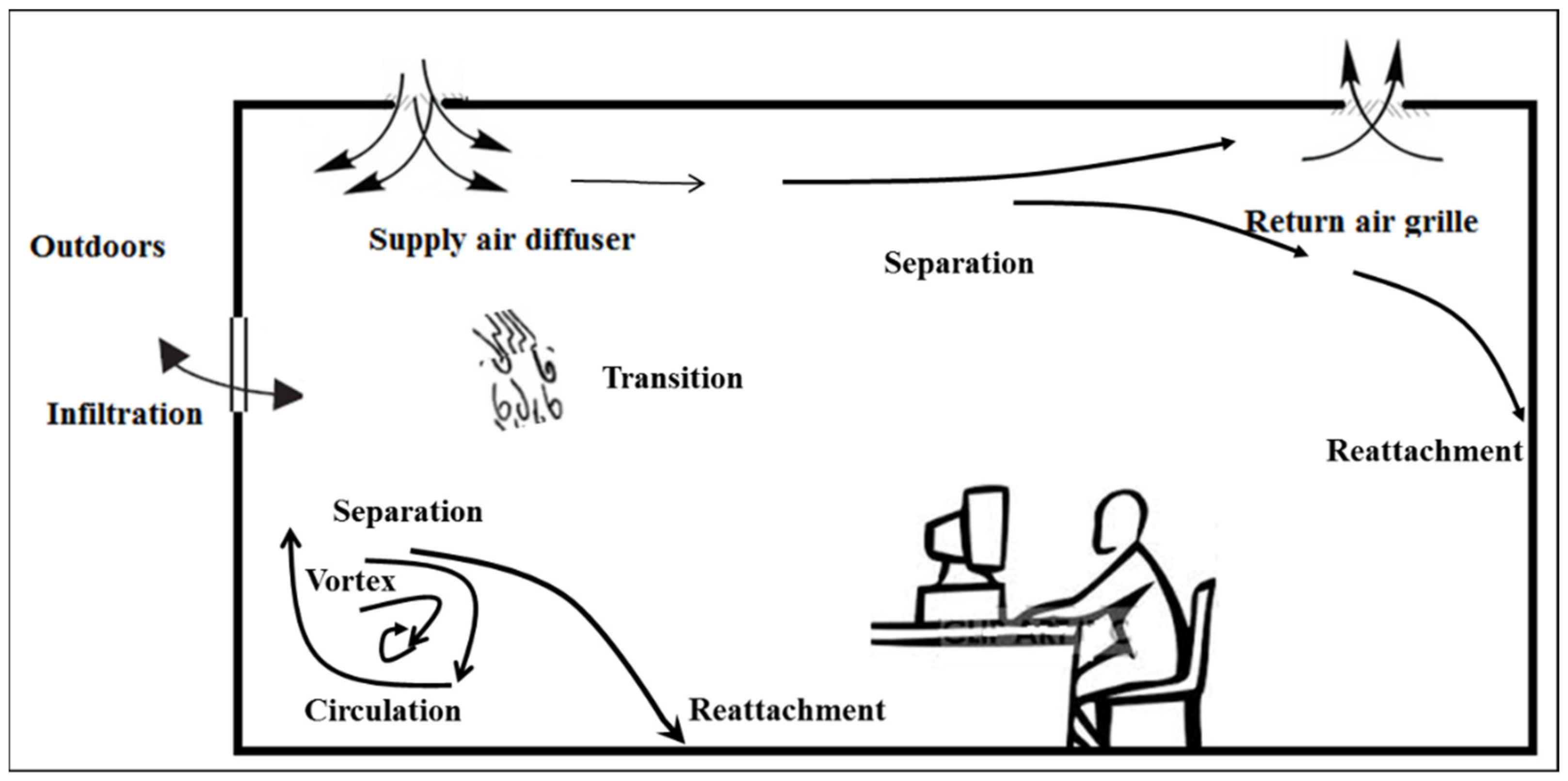
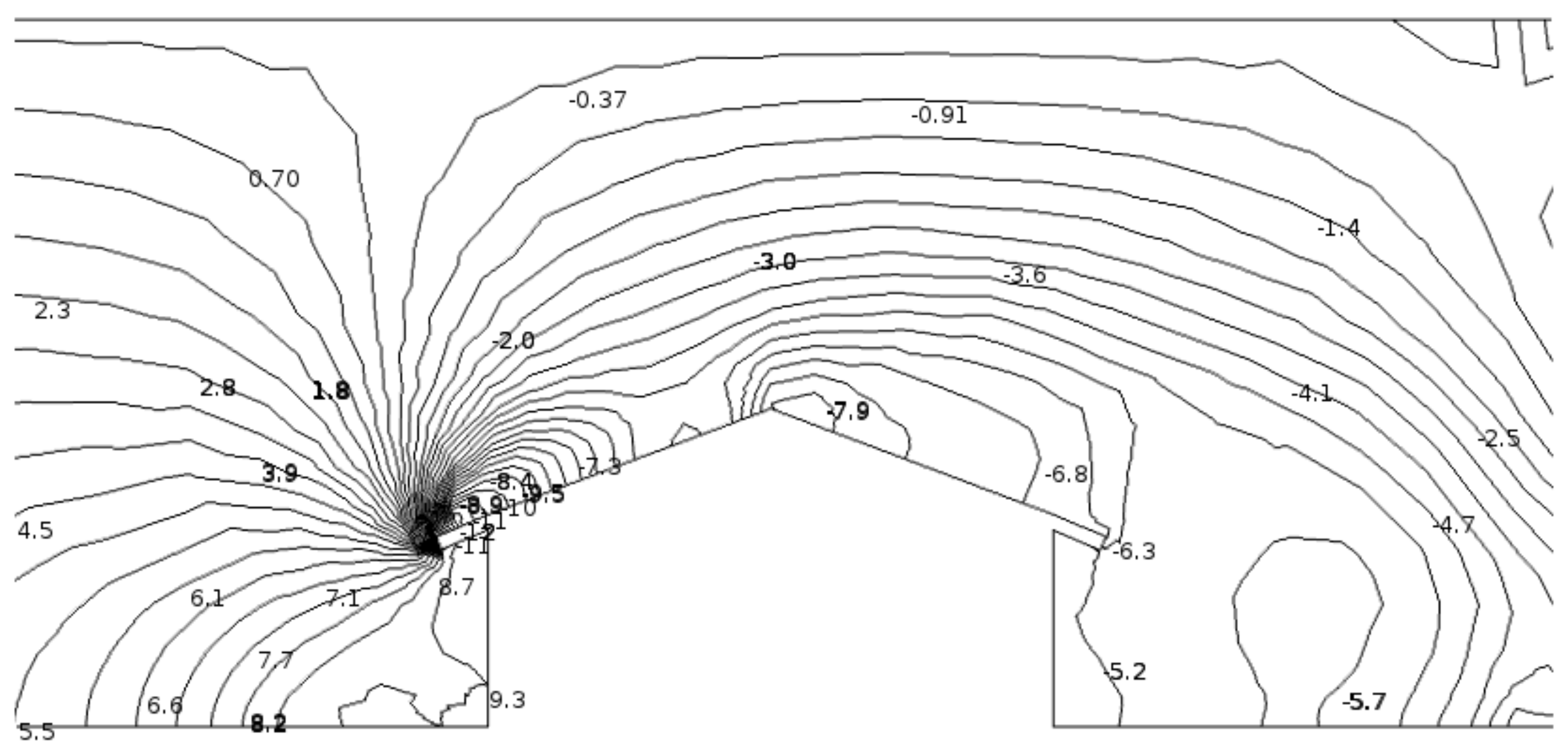
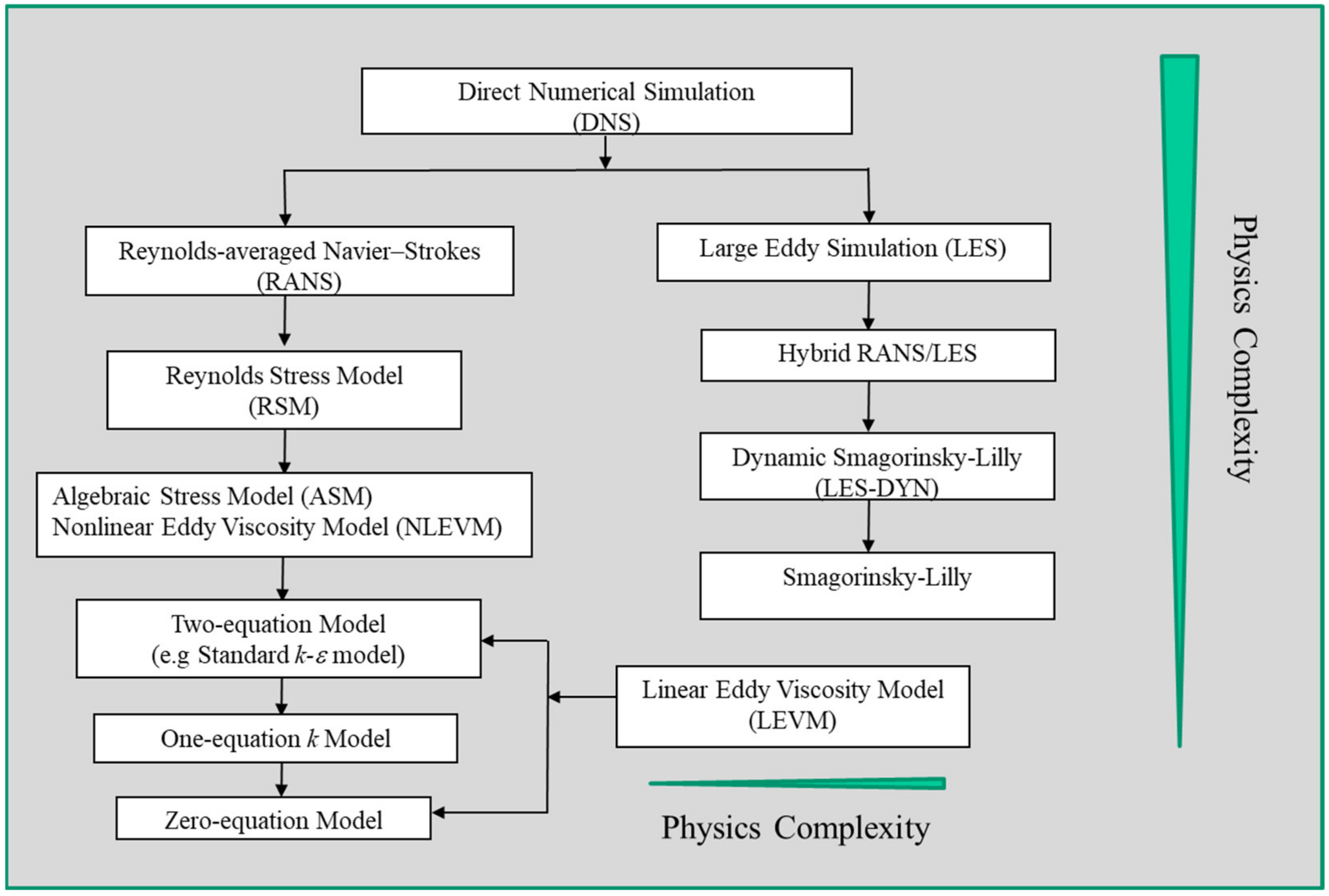
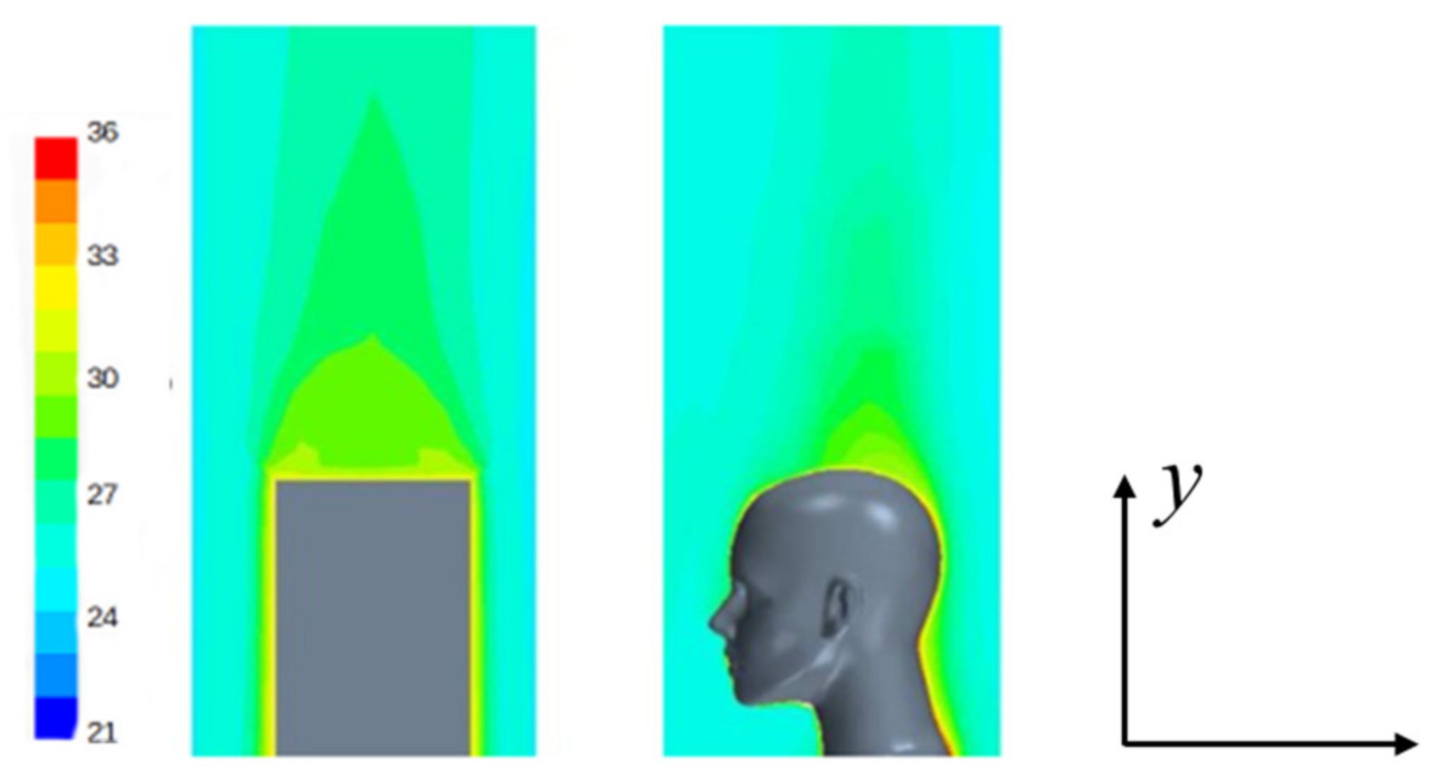
Table 1.
Comparison of DNS, LES, and RANS.
| DNS | LES | RANS | |
|---|---|---|---|
| Physics | full | high | low |
| Grids | Re9/4 | Re9/5 | log(Re) |
| Computations | ≥Re3 | Re2–Re25 | Re weakly |
| Applications | simple flow low Re number | simple flow low Re number | wide |
Table 2.
Examples of some commonly used commercial CFD software packages.
| Software | Sources | Locations |
|---|---|---|
| ANSYS CFX | ANSYS, Inc. | Canonsburg, PA, USA |
| Phoenics | CHAM Ltd. | London, UK |
| FLUENT | Fluent Inc. | Miami, FL, USA |
| CFX | ANSYS, Inc. | Canonsburg, PA, USA |
| OpenFOAM | OpenCFD Ltd. | Cannock, UK |
| COMSOL Multiphysics | COMSOL, Inc. | Burlington, MA, USA |
| STAR-CD | CD Adapco Group | Orlando, FL, USA |
| FLOW-3D | Flow Science, Inc. | Pasadena, CA, USA |
Table 3.
Application of RANS models in modeling COVID-19 virus transmission research.
| Models | Objectives | Articles |
|---|---|---|
| Zero-equation model | Examined the infection risks of the presidential debate by presidential candidates and the audience | [74] |
| Standard k-ε | Investigated spread of pathogenic species between occupants under different window configurations | [75] |
| RNG k-ε | Studied aerosol transport and surface deposition in classroom regarding effects of particle size, etc. | [76] |
| Realizable k-ε | Explored male-oriented urinal and the virus transmission | [77] |
| Standard k-ε | Explored and visualized toilet flushing and its influence on the spread of virus aerosol particles | [78] |
| Standard k-ε | Investigated inappropriate ventilation and the risk of airborne transmission of infectious diseases through virus-containing particles | [79] |
| Standard k-ε | Optimized air distribution for cross-infection control in hospital. Two newly developed parameters were proposed to give a quantitative evaluation of the air distribution | [80] |
| SST k-ω | Studied the cough’s droplet dispersion | [81] |
| SST k-ω | Tackled aerosol transport and deposition in human respiratory tract | [82] |
| Standard k-ε | Explored ultraviolet germicidal irradiation (UVGI) systems for reducing indoor bacterial concentration | [83] |
| Standard k-ε | Proposed safe classroom design regarding contagions and disease transmission | [84] |
Table 4.
Comparison of RANS models.
| Models | Simulation Application | Outperform Model | Articles |
|---|---|---|---|
| Standard k-ε, LRN, RNG k-ε | Natural, forced, and mixed convection in rooms | RNG k-ε model | [85] |
| LRN, RSM, standard k-ε | Indoor airflows and impinging flow | RSM (marginal) | [86] |
| Standard k-ε, RNG k-ε | Outdoor wind flow | RNG k-ε | [87] |
| Standard k-ε, RNG k-ε, LRN, standard k-ω, RSM | Ventilation and airflow in a farm house | RNG k-ε | [88] |
| Standard k-ε, RNG k-ε, RSM | Natural convection in a cubic cavity | Standard k-ε | [89] |
| RNG k-ε, RSM, SST k-ω | Turbulent flow inside an enclosure | SST k-ω | [90] |
| Standard k-ε, RNG k-ε, standard k-ω, SST k-ω, LES | Cross ventilation | LES, SST k-ω | [91] |
| Standard k-ε, RNG k-ε, SST k-ω, laminar model | Airflow in an office room | Standard k-ε, RNG k-ε, SST k-ω (marginal) | [92] |
| Standard k-ε, RNG k-ε, realizable k-ε | Airflow and heat transfer in a complex packaging facility | RNG k-ε | [93] |
| Standard k-ε, RNG k-ε, Realizable k-ε, SST k-ω, LRN, RSM | Indoor airflow | RNG k-ε, SST k-ω, LRN, RSM | [94] |
| Standard k-ε, RNG k-ε, realizable k-ε | Natural cross ventilation in a test chamber | RNG k-ε | [95] |
| Realizable k-ε, RNG k-ε, standard k-ω, SST k-ω | Mechanically ventilated enclosure | Standard k-ω | [96] |
| Zero-equation, RNG k-ε, LRN, SST k-ω, RSM, LES-DYN, DES | Indoor airflow | RNG k-ε, LES-DYN | [33] |
| One-equation, standard k-ε, RNG k-ε, realizable k-ε, standard k-ω, SST k-ω | Natural and forced convection in a ventilated facade | RNG k-ε | [97] |
| Zero-equation model, standard k-ε, RNG k-ε | Buoyancy-driven ventilation in atrium buildings | Zero-equation model | [98] |
| Standard k-ε, RNG k-ε, realizable k-ε, RSM, Smagorinsky model | Wind pressure around buildings | Smagorinsky model (RANS not accurate) | [99] |
| Standard k-ε, RNG k-ε, SST k-ω | Ventilated facade with phase change materials | RNG k-ε | [100] |
| Standard k-ε, RNG k-ε, standard k-ω, SST k-ω | Heat and airflow in room | RNG k-ε (marginal) | [101] |
| Standard k-ε, RNG k-ε, realizable k-ε, standard k-ω, the SST k-ω, RSM model | Airflow around buildings | SST k-ω overall | [102] |
| Standard k-ε, realizable k-ε, standard k-ω and SST k-ω | Wind flows around buildings | Standard k-ε, realisable k-ε | [103] |
Publisher’s Note: MDPI stays neutral with regard to jurisdictional claims in published maps and institutional affiliations. |
© 2021 by the authors. Licensee MDPI, Basel, Switzerland. This article is an open access article distributed under the terms and conditions of the Creative Commons Attribution (CC BY) license (https://creativecommons.org/licenses/by/4.0/).
Share and Cite
MDPI and ACS Style
Lü, X.; Lu, T.; Yang, T.; Salonen, H.; Dai, Z.; Droege, P.; Chen, H. Improving the Energy Efficiency of Buildings Based on Fluid Dynamics Models: A Critical Review. Energies 2021, 14, 5384. https://doi.org/10.3390/en14175384
AMA Style
Lü X, Lu T, Yang T, Salonen H, Dai Z, Droege P, Chen H. Improving the Energy Efficiency of Buildings Based on Fluid Dynamics Models: A Critical Review. Energies. 2021; 14(17):5384. https://doi.org/10.3390/en14175384
Chicago/Turabian StyleLü, Xiaoshu, Tao Lu, Tong Yang, Heidi Salonen, Zhenxue Dai, Peter Droege, and Hongbing Chen. 2021. "Improving the Energy Efficiency of Buildings Based on Fluid Dynamics Models: A Critical Review" Energies 14, no. 17: 5384. https://doi.org/10.3390/en14175384
Note that from the first issue of 2016, this journal uses article numbers instead of page numbers. See further details here.