
Positive Correlations between Short-Term and Average Long-Term Fluctuations in Wind Power Output
by
 , and
, and
Chiyori T. Urabe
1,* ,
,
Tetsuo Saitou
1,†,
Kazuto Kataoka
1,
Takashi Ikegami
2 and
Kazuhiko Ogimoto
1 1
Institute of Industrial Science, The University of Tokyo, Tokyo 1538505, Japan
2
Division of Advanced Mechanical Systems Engineering, Institute of Engineering, Tokyo University of Agriculture and Technology, Tokyo 1848588, Japan
*
Author to whom correspondence should be addressed.
†
Current address: Renewable Energy Institute, Tokyo 1050001, Japan.
Energies 2021, 14(7), 1861; https://doi.org/10.3390/en14071861
Submission received: 27 February 2021
/
Revised: 17 March 2021
/
Accepted: 25 March 2021
/
Published: 27 March 2021
(This article belongs to the Section A3: Wind, Wave and Tidal Energy)
Abstract
:Wind power has been increasingly deployed in the last decade to decarbonize the electricity sector. Wind power output changes intermittently depending on weather conditions. In electrical power systems with high shares of variable renewable energy sources, such as wind power, system operators aim to respond flexibly to fluctuations in output. Here, we investigated very short-term fluctuations, short-term fluctuations (STFs), and long-term fluctuations (LTFs) in wind power output by analyzing historical output data for two northern and one southern balancing areas in Japan. We found a relationship between STFs and the average LTFs. The percentiles of the STFs in each month are approximated by linear functions of the monthly average LTFs. Furthermore, the absolute value of the slope of this function decreases with wind power capacity in the balancing area. The LTFs reflect the trend in wind power output. The results indicate that the flexibility required for power systems can be estimated based on wind power predictions. This finding could facilitate the design of the balancing market in Japan.
1. Introduction
For improved environmental sustainability, renewable energy generators have been widely deployed all over the world. At the 21st session of the Conference of the Parties, participating countries agreed to find a balance between sources and sinks of greenhouse gases in the second half of this century. These countries are required to meet aggressive targets to reduce greenhouse gas emissions [1].
Renewable energy generation is effective for reducing greenhouse gas emissions in the electricity sector. The International Energy Agency and the International Renewable Energy Agency reported that the share of renewable energy needs to increase from about 15% of the primary energy supply in 2015 to 65% in 2050 to accomplish the stated goals [2]. Wind and solar power provide a large proportion of variable renewable energy (VRE) [3]. In Japan, the installed capacity of wind power was GW in 2010 and GW in 2019 [4]. According to the Long-term Energy Supply and Demand Outlook report published by the Ministry of Economy, Trade and Industry, Japan, the target for wind power installation by 2030 is 10 GW [5]; according to a report by the Japan Wind Power Association, the target for 2050 is 75 GW [6].
VRE power output changes intermittently, depending on the weather conditions. Fluctuations in VRE power outputs can negatively impact the operation of a power system [7,8,9,10,11,12]. A power system operator requires flexibility to compensate for these fluctuations. Traditionally, the system operator controls power outputs from conventional power plants to maintain the balance between supply and demand, which is a source of flexibility. Growth of the share of VRE in the power supply increases the impact of fluctuations in VRE output on system operation. Mitigation of these fluctuations and provision of flexibility are urgent issues that must be addressed to accelerate the use of VRE resources. The issue of power system flexibility has been discussed by committees within the Organization for Cross-regional Coordination of Transmission Operators, Japan (OCCTO) [13]. Recently, OCCTO has been studying the design of a new balancing market to ensure flexibility [14].
Understanding fluctuations in VRE outputs helps system operators to efficiently respond to them. From the perspective of system operation, fluctuations in demand and VRE outputs can be considered according to a few timescales. According to the European Network of Transmission System Operators and OCCTO, fluctuations are compensated by primary, secondary, and tertiary reserves [14,15]. In this paper, we focus on fluctuations in wind power output and distinguish among historical data on very short-term fluctuations (VSTFs), short-term fluctuations (STFs), and long-term fluctuations (LTFs). VSTFs and STFs have timescales of less than 1 min and several tens of minutes, respectively. LTFs indicate the trend of wind power output.
Fluctuations in wind power outputs have been defined and analyzed by several methods [7,8,9,16,17,18,19,20,21,22,23,24,25,26,27]. The fluctuations depend on the season and balancing area (BA). In several BAs, the fluctuations tend to increase in winter [26]. A geographical spread of wind power plants (WPPs) mitigates these fluctuations [8,16,18,19,20,21,22,23,24,25,26,27,28,29,30,31,32], which is called the smoothing effect. In addition, the smoothing effect in a single WPP was also investigated and facilitated smoothing the fluctuations in wind power output in BAs [33,34,35,36]. While the smoothing effect in a WPP amplifies with the number of wind turbines [33], a large WPP with many wind turbines can induce rapid decreases of wind power output by storms, especially in countries and regions where multiple typhoons approach every year. It is difficult to generalize the characteristics of the fluctuations in wind power output. However, generalized characteristics of system operation could be improved.
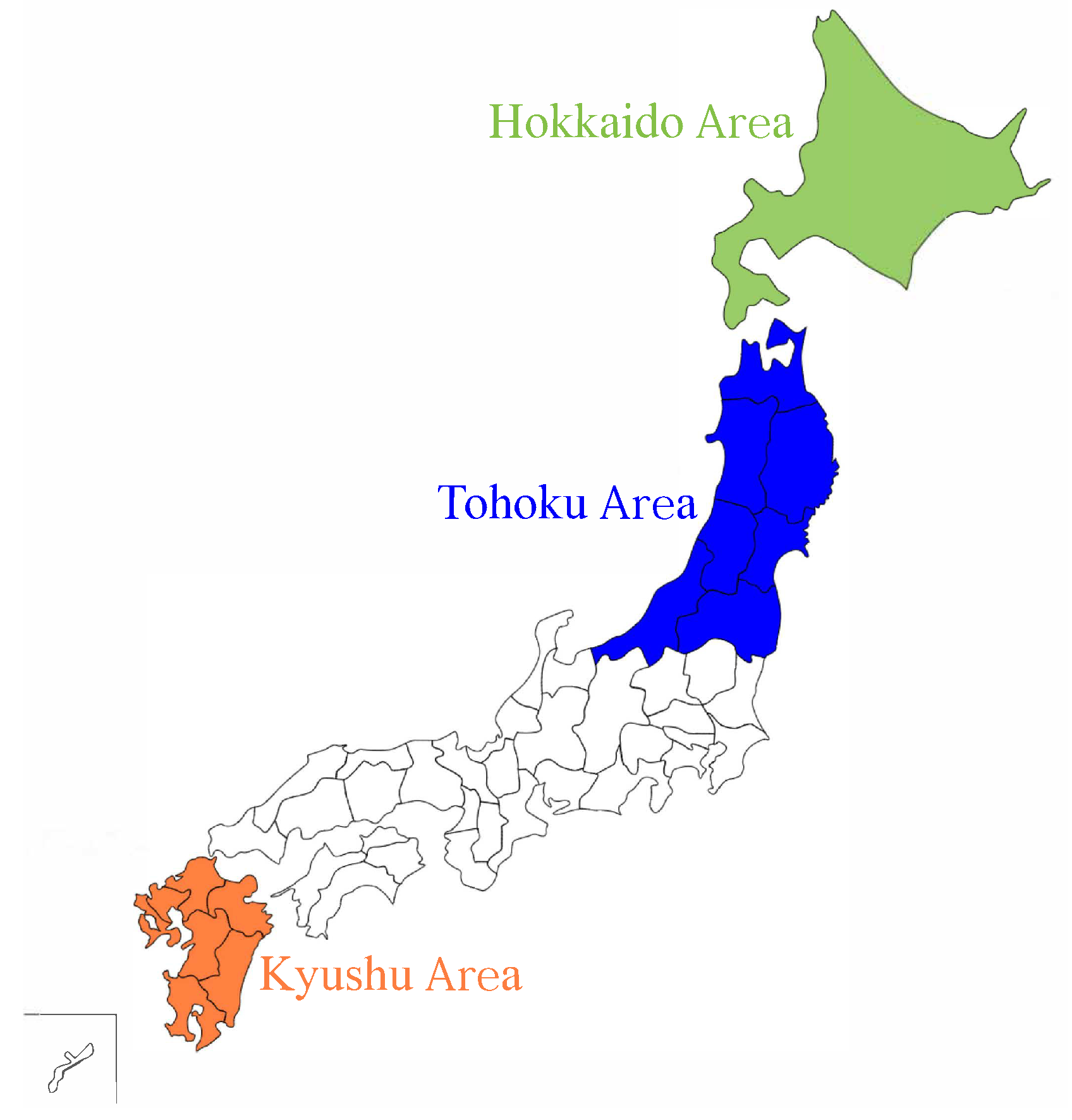
In Japan, there are 10 BAs. The northern BAs have a different pattern of fluctuations in wind power output than the southern ones. We analyzed fluctuations in three Japanese BAs, i.e., those of Hokkaido, Tohoku, and Kyushu, as shown in Figure 1. While the Hokkaido and Tohoku areas have many windy days in winter, the seasonal pattern is different in Kyushu. The STFs in the Hokkaido area have larger amplitudes than those in the other two BAs. The Tohoku area has smaller-amplitude STFs than the other two BAs. Although the seasonality and fluctuations differ among these three BAs, we found that they were similar with respect to the relationship between STFs and LTFs. The relationship is approximately a linear function, in which the STFs increase with the monthly average of the LTFs. In addition, the absolute value of the slope of each linear function decreases with the wind power capacity of the BA.
The relationship between the STFs and LTSs was revealed through this study and could influence the smoothing effect [8,16,18,19,20,21,22,23,24,25,26,27,28,29,30,31,32,33,34,35,36]. Thus, the large LTFs, which increase the STFs, could reduce the smoothing effect in the STFs. However, if the monthly wind power output is estimated using historical output and weather data, a system operator could more accurately estimate the reserves that are necessary to procure against the STFs in the wind power output of each BA. The secondary reserves respond to the STFs in wind power output and consist mostly of rapidly starting gas turbine power plants, hydro storage plants, and load shedding [37], while the hydro storage plants and power system planning cater to the LTFs. Information about STFs in wind power output could facilitate the design of a new balancing market that ensures the required reserves [14,38].
This paper is organized as follows. Section 2 and Section 3 describe the historical data on wind power output used for our analysis of fluctuations and the methodology used to distinguish among the different sorts of fluctuations, respectively. Section 4 presents the results, and Section 5 is devoted to discussion and conclusions.
2. Historical Data of Wind Power Outputs
Historical data on the total wind power output in three BAs were used: Hokkaido, Tohoku, and Kyushu. These three BAs are considered to have high potential for wind power resources [39]. The wind power capacities of these BAs are listed in Table 1. The capacity of the Hokkaido area was smallest, being less than half that of Tohoku, which has the largest capacity and highest number of WPPs. Kyushu is intermediate in terms of capacity and number of WPPs.
The time periods of the data are 1 fiscal year (FY), FY2012, in the Hokkaido and Kyushu areas, and 3 years, FY2010–FY2012, in the Tohoku area. A FY in Japan is from 1 April to 31 March. The data have small time resolutions, less than 10 s, allowing analysis of the VSTFs and STFs, whose periods are less than 1 min and several tens of minutes, respectively.
Some of the raw data for the wind power outputs were missing. When the period of missing data was less than 3 h, the missing data were linearly interpolated. Missing data with longer periods were removed from the time series, as listed in Appendix A.
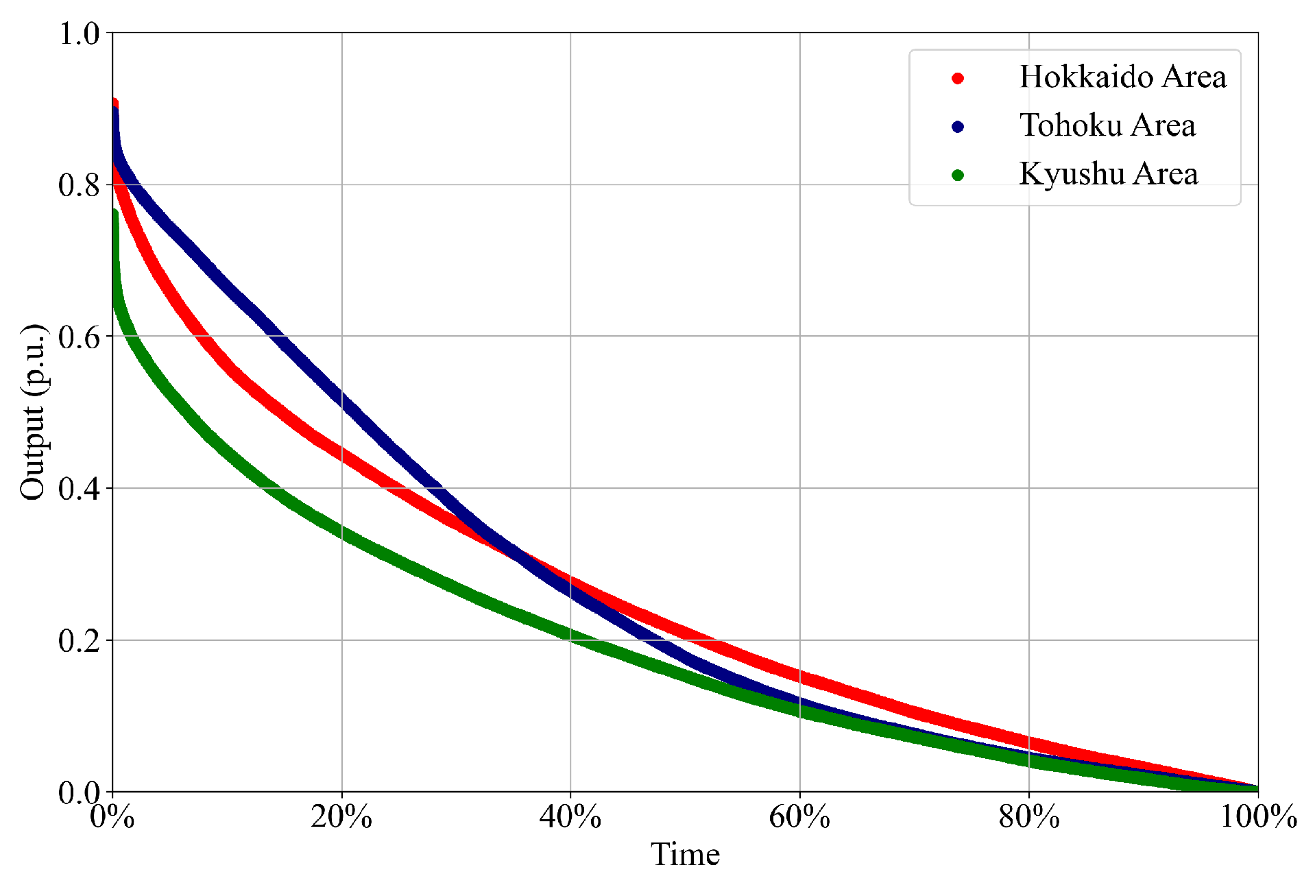
The data were analyzed in terms of per unit (p.u.) values, which indicate the ratio of wind power output to capacity. While the ideal maximum output corresponds to 1 p.u., the actual total output never reaches this level because of the smoothing effect. Figure 2 shows the duration curves of the wind power output in the Hokkaido, Tohoku, and Kyushu areas in FY2012. The maximum output was approximately p.u. The Kyushu area had smaller outputs than Hokkaido and Tohoku.
3. Methods
Traditionally, in Japanese electrical power systems, STFs in electricity demand have been defined within 20-min windows. STFs in wind power output have been analyzed in terms of standard deviation (SD), differences among several timeframes, power spectra, and wavelets; their static features have also been discussed [16,19,26,32,40,41,42,43]. While analysis methods based on SDs and differences in timeframes are computationally cheap, they cannot separate time series of wind power outputs into time series of different sorts of fluctuations. Methods based on power spectra and wavelets can provide detailed information about fluctuations; however, the computational costs of these methods are too large for applications in real-time system operation.
In this paper, we focus on STFs in wind power output to promote the use of wind power in power systems, while avoiding any negative impact of this power source on system operation. The methods used to distinguish STFs in wind power outputs must be computationally cheap and provide detailed information. A method with centered moving averages (CMAs) is adopted, which is described later [26].
Regardless of the differences in the methods mentioned above, some common characteristics of STFs have been reported: smoothing effects mitigate STFs [16,32] and STFs have non-Gaussian distributions with heavy tails [26,43].
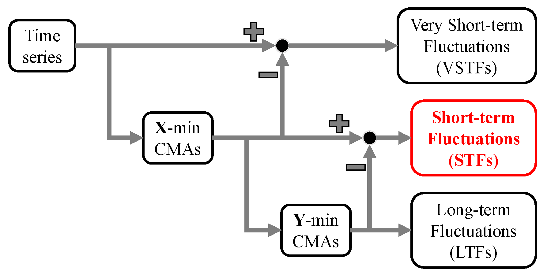
3.1. Separation Method for LTFs, STFs, and VSTFs in Wind Power Outputs
The method using CMAs is summarized in Figure 3. The time series of wind power output is separated into VSTFs, STFs, and LTFs by this method. The timescale of VSTFs is determined by a parameter, X; the time resolution of the wind power output must be shorter than this timescale. Likewise, the timescales of STFs and LTFs are determined by X and Y. X has only positive values and must be sufficiently smaller than Y.
The X and Y CMAs, and , respectively, are defined as follows:
where represents the wind power output at time t and and are the numbers of data points in time periods X and Y (in minutes), respectively.
VSTFs, STFs, and LTFs are represented by and , respectively, as follows:
, , and can reproduce the original time series as follows: . Therefore, no information is lost during the separation process.
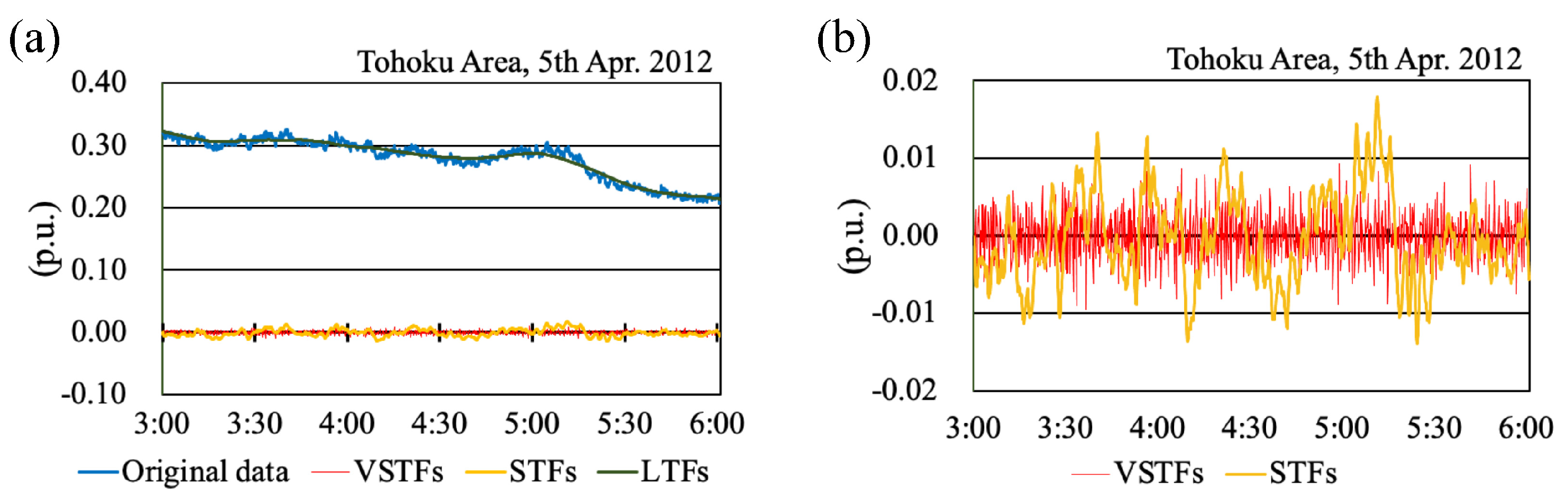
Figure 4 shows the time series of VSTFs, STFs, and LTFs. X and Y in Figure 3 and Equations (1)–(3) are fixed to 1 and 30 min, respectively. The validity of this parameter setting is discussed in the next subsection. Figure 4a includes the time series of , LTFs, STFs, and VSTFs. LTFs represent the trend of and change smoothly; they have larger amplitudes than those of VSTFs and STFs. In Figure 4b, note that the STFs and VSTFs change around a value of zero. STFs tend to have larger amplitudes and longer cycles than VSTFs.
3.2. Basic Properties of LTFs, STFs, and VSTFs
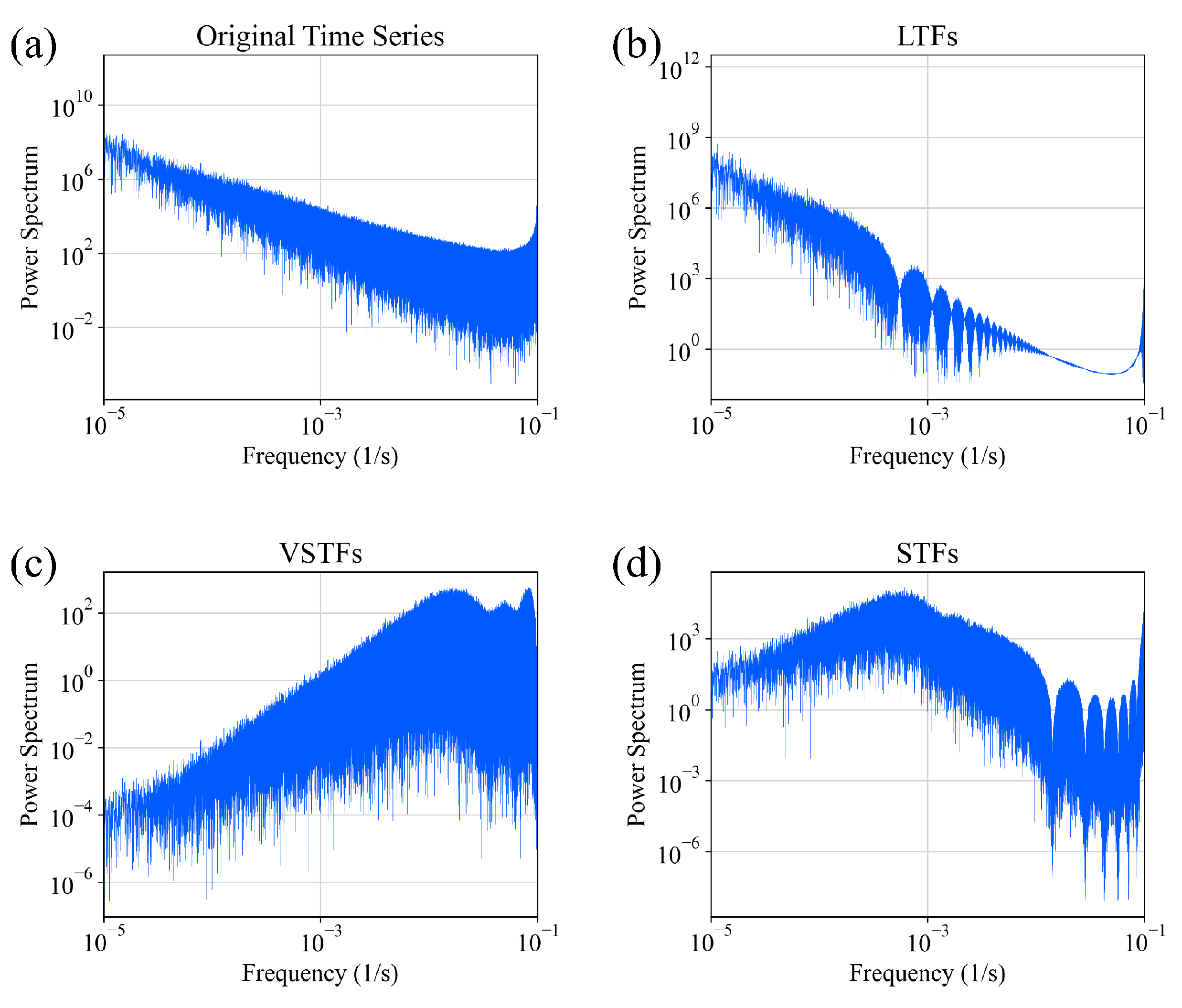
Figure 5 shows the power spectra of the time series of , LTFs, STFs, and VSTFs in the Tohoku area in FY2012. Comparing Figure 5a,b indicates that the power spectrum of the LTFs has a similar trend to that of . However, the power spectrum of the LTFs has a steeper slope than that of because the separated VSTFs and STFs are removed. The power spectra of the VSTFs and STFs have peaks after around several tens of seconds and minutes, as can be seen in Figure 5c,d, respectively.
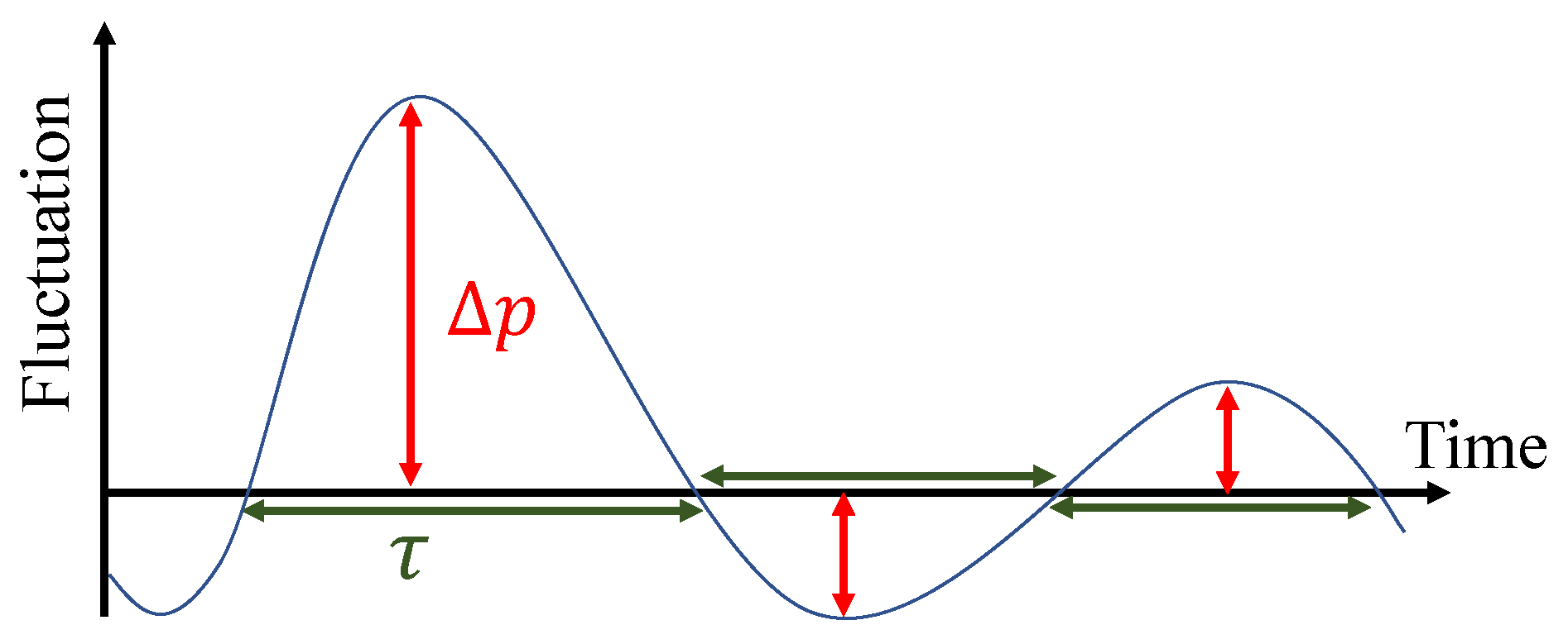
Microscopically, the time series of STFs consist of multiple half-cycles. Each half-cycle has an amplitude, , and a period, , as shown in Figure 6, which contains more than three half-cycles. The timescale of STFs is double the length of , thus, the period of a whole cycle.
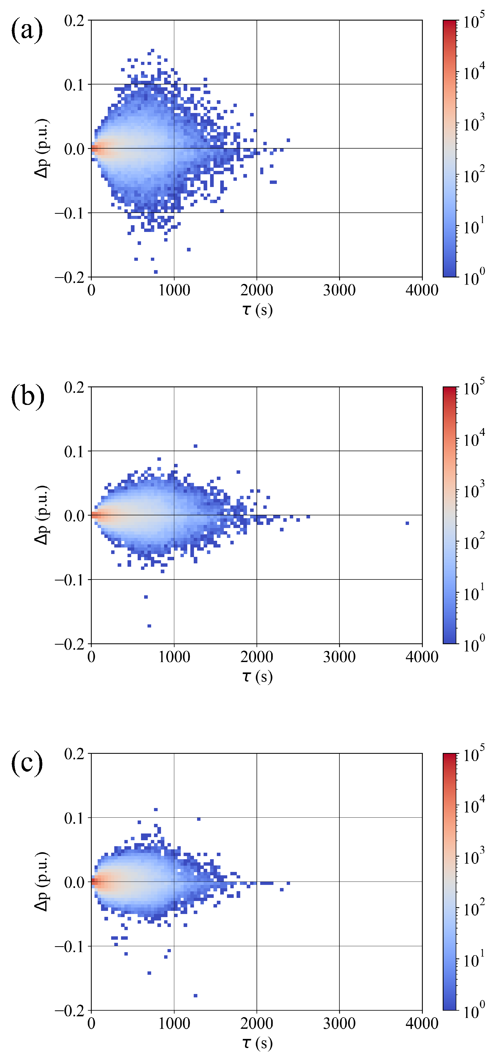
The distributions of and in the three BAs are shown in Figure 7. The values involving the maximum in each BA occur at approximately 15 min. Thus, the cycle period that could have the maximum impact on power systems is approximately 30 min. The maximum values in the Hokkaido area tended to be the largest ones among the three BAs. Conversely, the values in the Kyushu area were relatively small.
In this paper, STFs are defined as fluctuations that have a timescale of several tens of minutes. The parameters were set to min and min in Figure 3 and Equations (1)–(3), and analyzed STFs based on the power spectra, , and . In our first analysis, there were a number of STFs with values of several tens of minutes. Other analyses showed that STFs with the highest have periods of approximately 30 min. We consider that appropriate parameter settings can provide STFs consistent with this definition.
4. Results
4.1. Statistical Properties of STFs
Some statistical properties of STFs in the Hokkaido, Tohoku, and Kyushu areas in FY2012 are listed in Table 2. Comparing the three BAs, the Hokkaido one has the highest SD and percentile values. The Kyushu area has a smaller SD and the 1st and 99th percentile values than Tohoku. These results are consistent with the trend shown in Figure 7.
The Pearson product–moment correlation coefficients between STFs with VSTFs and LTFs provide information about correlations at the same time and are defined as follows:
, , and are the averages of , , and during , where is the time step, 3 s in the Hokkaido area, 10 s in the Tohoku area, and 2.5 s in the Kyushu area; N is the number of data. Correlation coefficients of STFs with VSTFs and LTFs, CC and CC, respectively, in Table 2, indicate that the correlations are small; thus, STFs are effectively not correlated with VSTFs or LTFs.
On the other hand, we can deduce that there is some relationship between LTFs and STFs, as follows. When LTFs in are small, itself must also be small. When is small (large), the possible decrement (increment) of STFs at the next time step is limited by the wind power output at that time. Therefore, we infer that the LTFs affect STFs.
4.2. Distributions of STFs and LTFs
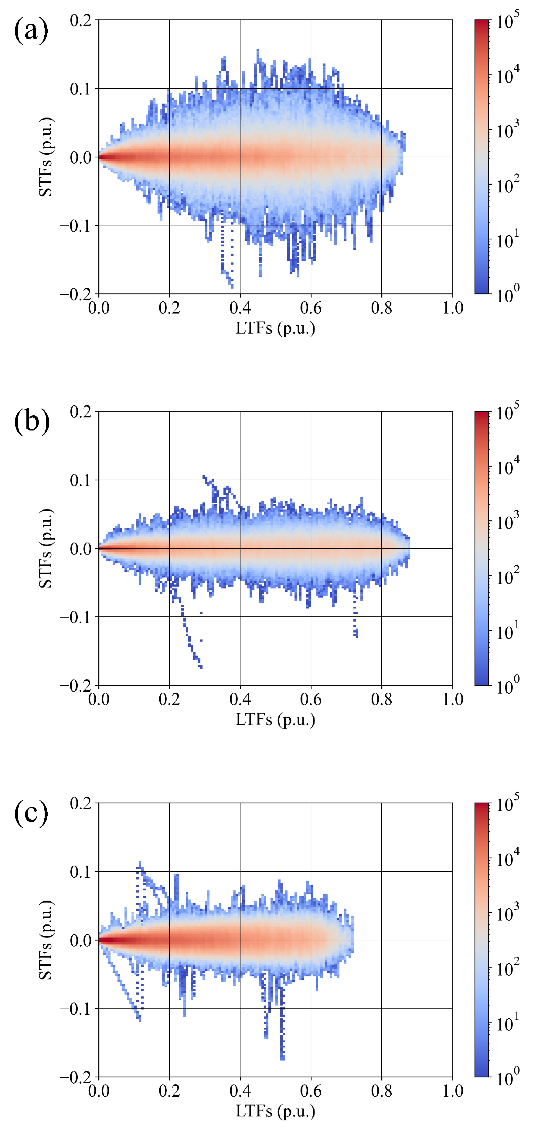
To determine if there was any relationship between STFs and LTFs, we investigated their distributions. Scatter diagrams of STFs versus LTFs in FY2012 are shown in Figure 8. In the three BAs, when LTFs are small, the of the STFs are also small. The high-density areas, which are colored red, are approximately elliptical in shape in all three BAs, with the height and width of the ellipse differing according to the BA. The ellipse is largest for the Hokkaido area, indicating that it had the largest for STFs. Although the Tohoku area has LTFs of approximately the same width of those of the Hokkaido area, the of its STFs tended to be smaller than those in Hokkaido, except for a few long lines around the ellipse.
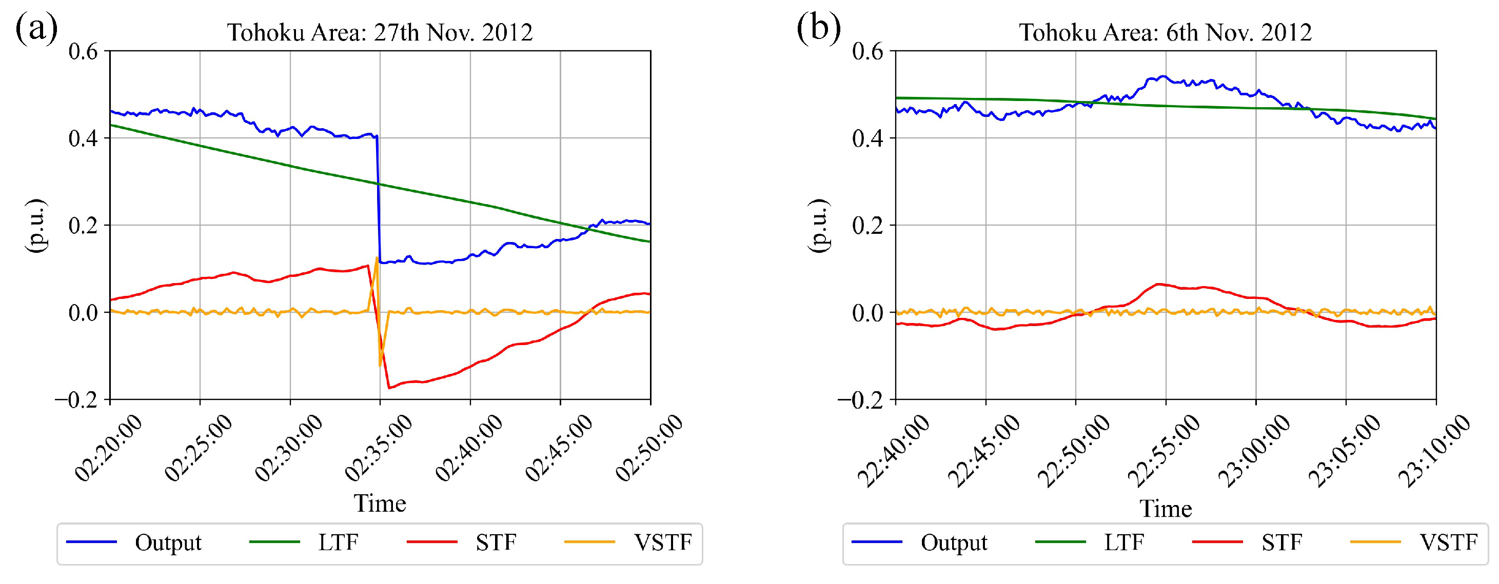
In Figure 8, there are several long lines around the ellipses. Each continuous line indicates a single event during which increased or decreased drastically. In the Hokkaido and Tohoku areas, these events tended to occur in winter. In the Tohoku area, two events in November induced the largest and smallest STFs; these events are depicted in Figure 9. In both cases, multiple low-pressure systems passed near the Tohoku area [44] and we infer that these caused the events. The event on 27 November, shown in Figure 9a, resulted from the wind turbines in multiple WPPs cutting out [26]. Wind turbines cut out to avoid damage when the wind speed exceeds 25 m/s.
4.3. Seasonality of STFs
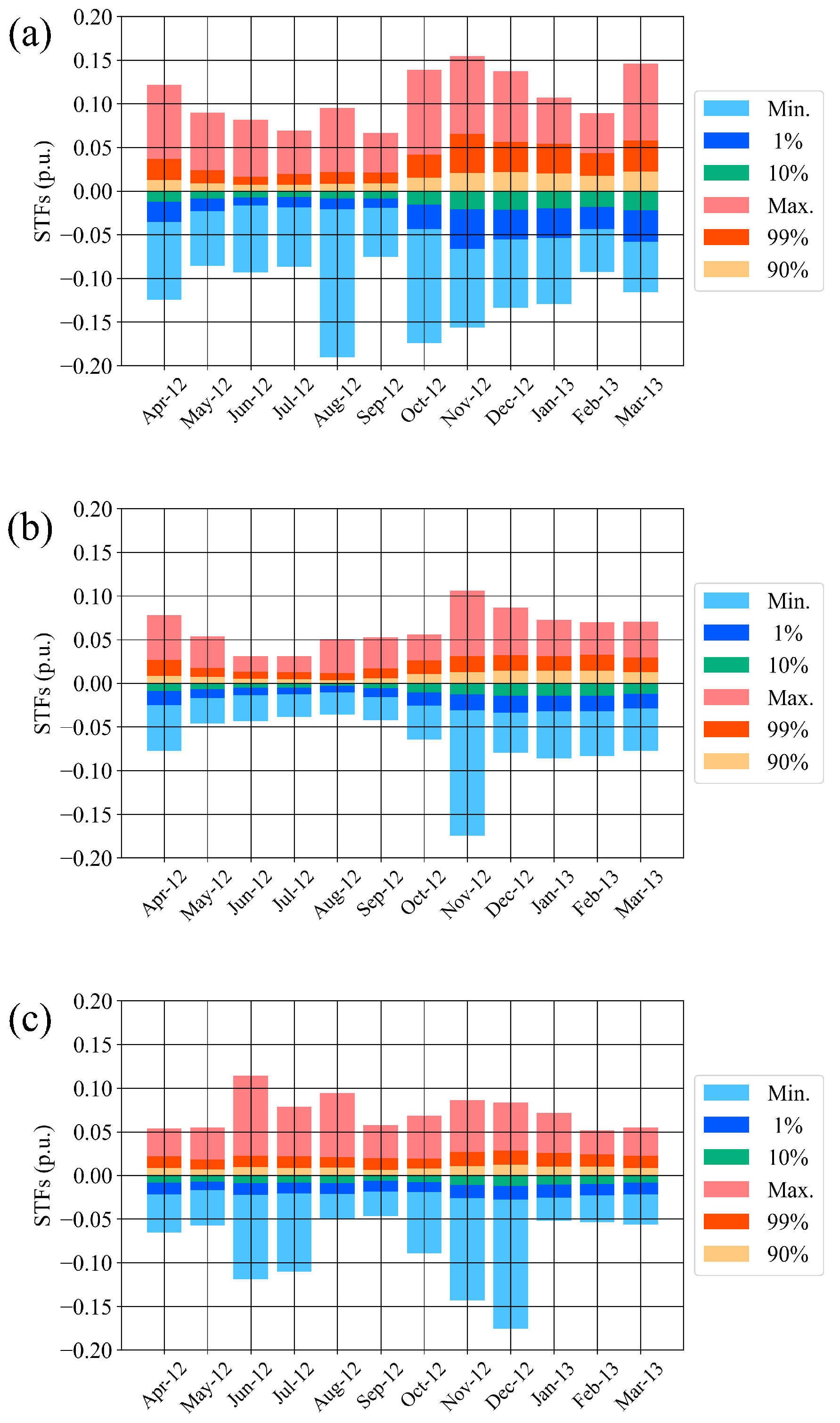
Figure 10 shows the maximum, minimum, and percentiles of SFTs in each month in FY2012. While the maximum and minimum in each month are strongly affected by single significant events, the percentiles depend on multiple events. Therefore we focus on these in this paper, especially the 10th and 90th ones.
In the Hokkaido and Tohoku areas, the percentiles have larger amplitudes in winter, from November to February. The percentiles for the Kyushu area are approximately the same across FY2012. The STFs in the Tohoku area in FY2010 and FY2011 also tended to be larger in winter, as shown in Figure 11. From FY2010 to FY2012, its STFs were smaller from June to August.
4.4. Relationship between STFs and Average LTFs
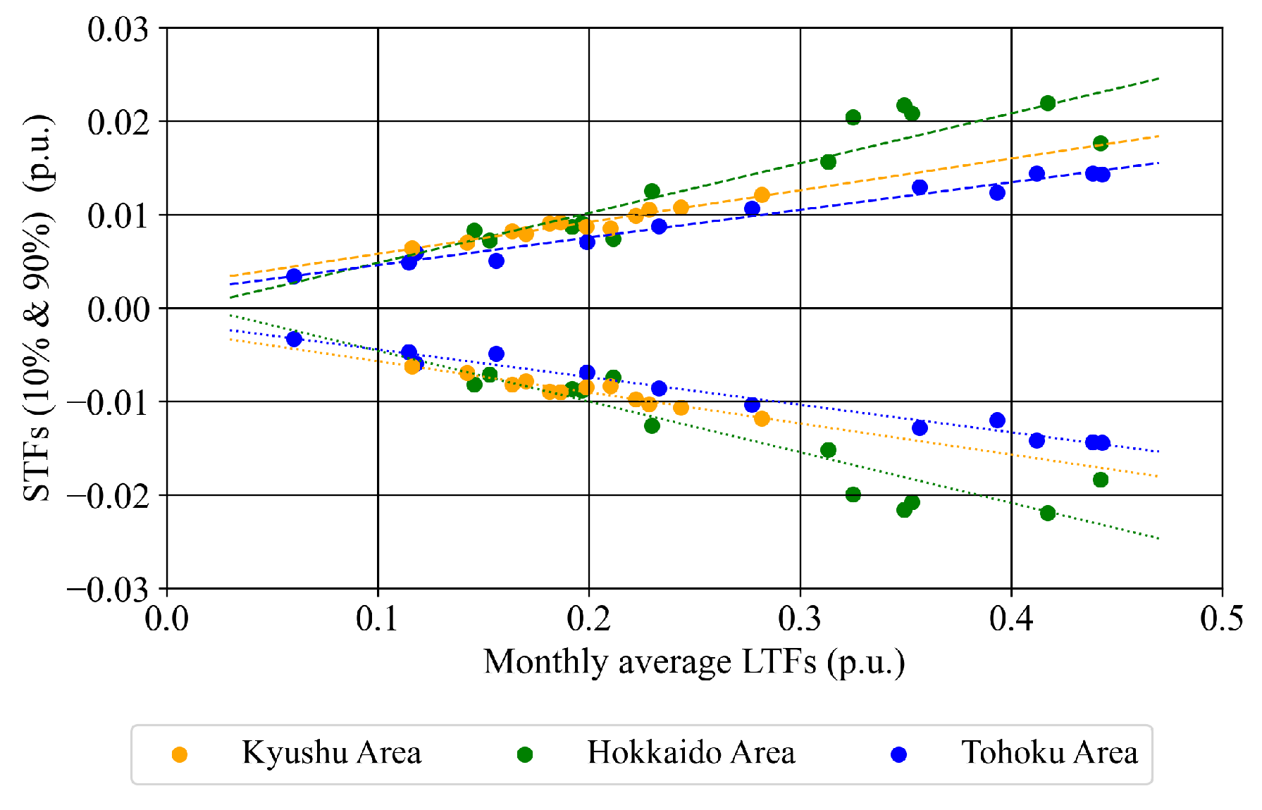
Although the correlation coefficient between STFs and LTFs is small, as shown in Table 2, in the Hokkaido and Tohoku areas, the of STFs tended to increase in winter when increased [45], as shown in Figure 10 and Figure 11. Hence, we inferred that there is some relationship between STFs and .
To reveal the relationship between STFs and LTFs, which indicate the trend in , in Table 3, we list the correlation coefficients between the monthly 10th and 90th percentiles of STFs and average LTFs. These coefficients in each BA are sufficiently large to indicate that there is a correlation.
In Figure 12, we show the relationship between the 10th and 90th percentiles of STFs and the average LTFs in each month, for the three BAs in FY2012. Each data point represents one monthly percentile for one BA, thus, there are 72 dots in the figure, with those above (below) the horizontal axis representing the 90th (10th) percentile. For all BAs, the STF percentiles increased with the monthly average LTFs, with the dashed lines indicating functions obtained by least-squares approximation of the percentiles in each BA. The slopes of the lines for the Hokkaido area have the largest absolute values, with those of Tohoku being the smallest.
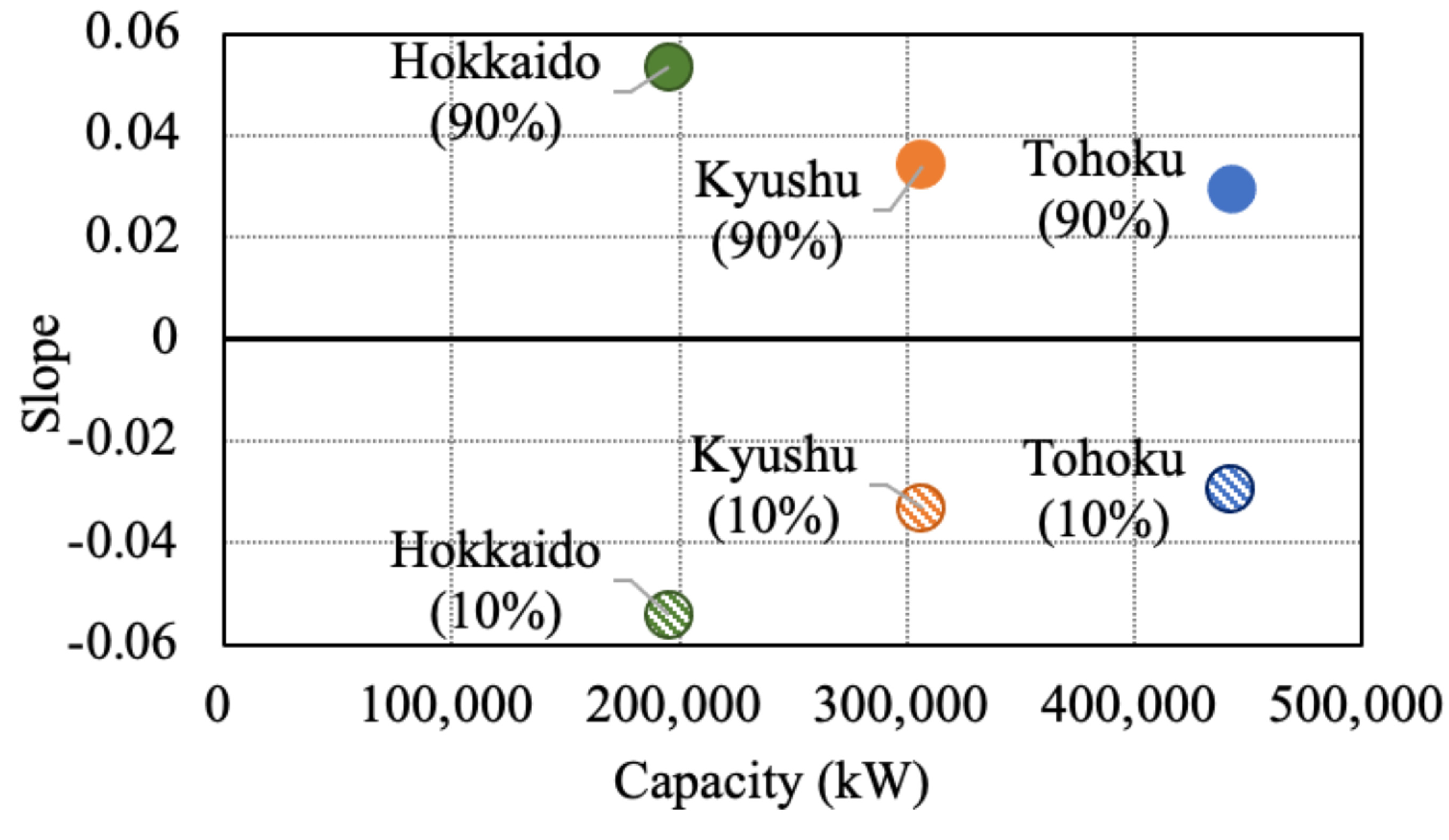
The absolute values of the slopes tend to decrease with wind power capacity, as shown in Figure 13. While the capacity in the Hokkaido area was less than half that in the Tohoku area, the absolute values of the slopes for Tohoku were larger than half of those for Hokkaido. We expect that the absolute values of these slopes would not become zero even if the capacity were exceptionally large. Therefore, the absolute values of the slopes would decrease asymptotically to nonzero values.
5. Discussion and Conclusions
A high share of wind power generation in a power system can amplify the negative impact of fluctuations in on system operation. To respond to these fluctuations, a system operator prepares reserves with different timescales. While the fluctuations in are mitigated though the smoothing effect [8,16,18,19,20,21,22,23,24,25,26,27,28,29,30,31,32], large fluctuations can remain when a BA is restricted to a small area and has insufficient interconnections with other BAs. Japan has 10 BAs and an inhomogeneous distribution of potential wind resources. Therefore, to promote wind power generation in Japan, mitigation of the fluctuations in is an urgent issue.
The fluctuations are separated into VSTFs, STFs, and LTFs, depending on their timescale. VSTFs and STFs have timescales of less than 1 min and several tens of minutes, respectively. LTFs have the longest timescale, of more than 1 h. In this paper, time series of are separated into VSTFs, STFs, and LTFs via a method based on CMAs [26].
We analyzed historical data for in three BAs, i.e., Hokkaido, Tohoku, and Kyushu, in Japan in terms of their fluctuations. The Hokkaido and Tohoku areas are in the northern region on the main island of Japan, while the Kyushu area is mainly on Kyushu Island, which is south of the main island. The northern BAs, Hokkaido and Tohoku, have a different pattern of fluctuations from Kyushu, where the and of their STFs tend to be large in winter and decrease in summer.
The LTFs of indicate the trend in . We investigated the relationship between STFs and LTFs and found that the 10th and 90th percentiles of the STFs in each month increased with the monthly average LTFs in all three BAs. The relationship between the STF percentiles and the average LTFs in each BA can be approximated by a linear function. Additionally, the absolute value of the slope of this function decreases with the wind power capacity in a BA. This result provides an indication of the reserves required to respond to STFs in in each BA.
Recently, OCCTO has been working on a new balancing market for Japan [14]. Information about fluctuations in could contribute to efficient procurement of reserves for the planned market, to promote the penetration of wind power while avoiding the negative impact of fluctuations in on the power system. We consider that information about fluctuations is essential for designing the new balancing market. According to the relationship between the STFs and LTFs, the STFs can amplify and require more reserves when wind power output increases, thus, when the LTFs are expected to increase. The new balancing market should be designed to ensure required reserves, and system operators use the reserves to respond to the STFs. In future work, we plan to develop a wind power control method to mitigate STFs therein.
Author Contributions
Conceptualization, C.T.U., T.S., K.K., T.I. and K.O.; data curation, C.T.U., T.S., T.I. and K.O.; formal analysis, C.T.U. and T.S.; methodology, C.T.U., T.S., K.K. and T.I.; software, C.T.U.; writing–original draft, C.T.U.; writing–review & editing, C.T.U., T.S., K.K., T.I. and K.O. All authors have read and agreed to the published version of the manuscript.
Funding
This paper is based on results obtained from a project commissioned by the New Energy and Industrial Technology Development Organization (NEDO).
Data Availability Statement
The data presented in this study are available on request from the corresponding author. The data are not publicly available because they include information about the non-public corporate profits of WPP owners.
Conflicts of Interest
The authors declare no conflict of interest.
Abbreviations
The following abbreviations are used in this manuscript:
| BA | Balancing area |
| CMA | Centered moving average |
| FY | Fiscal year |
| LTF | Long-term fluctuation |
| OCCTO | Organization for Cross-regional Coordination of Transmission Operators, Japan |
| SD | Standard deviation |
| STF | Short-term fluctuation |
| VRE | Variable renewable energy |
| VSTF | Very short-term fluctuation |
| WPP | Wind power plant |
Appendix A. Missing Data List
Sequences of missing data longer than 3 h were removed from the original time series of . The missing data are listed in Table A1. We defined the rate of loss as the proportion of 1 year that the missing data covered. In the Hokkaido area, the missing data were caused by signal transfer errors from WPPs to the data aggregation system. In the Tohoku area, there were two sequences of missing data: from 11 to 12 March 2011 and from 7 to 8 April 2011. Earthquakes caused these losses; the former began just after the Great East Japan Earthquake on 11 March 2011, and the latter began just after an aftershock of the earthquake.

Table A1.
Missing data of longer than 3 h.
| Balancing Area | Fiscal Year | Missing Data | Rate of Loss |
|---|---|---|---|
| Hokkaido | 2012 | 2013-01-14 9:28:12–2013-01-24 14:02:03 | 12.5% |
| 2013-02-11 9:26:06–2013-03-18 23:56:57 | |||
| Tohoku | 2010 | 2011-03-11 14:47:10–2011-03-12 17:16:10 | 0.3% |
| Tohoku | 2011 | 2011-04-07 23:34:00–2011-04-08 8:51:40 | 0.1% |
| Tohoku | 2012 | NA | 0.0% |
| Kyushu | 2012 | NA | 0.0% |
NA: Not Applicable. *1 Caused by the Great East Japan Earthquake on 11 March 2011. *2 Caused by an aftershock
of the Great East Japan Earthquake.
References
- INDCs as Communicated by Parties. Available online: http://www4.unfccc.int/submissions/indc/Submission%20Pages/submissions.aspx (accessed on 28 January 2021).
- International Energy Agency (IEA); International Renewable Energy Agency (IRENA). Perspectives for the Energy Transition; IEA Publications and IRENA Publications: Footscray, Australia, 2017. [Google Scholar]
- Renewables 2017 Global Status Reports. Available online: http://www.ren21.net/wp-content/uploads/2017/06/17-8399_GSR_2017_Full_Report_0621_Opt.pdf (accessed on 26 January 2018).
- Installed Capacity of Wind Power in Japan (Flash Report at the End of 2019). Available online: http://jwpa.jp/pdf/dounyuujisseki2019graph.pdf (accessed on 28 January 2021). (In Japanese).
- Long-Term Energy Supply and Demand Outlook. Available online: http://www.enecho.meti.go.jp/category/others/basic_plan (accessed on 28 January 2021). (In Japanese).
- Vision (Mid/Long-Term Installation Goals). Available online: http://jwpa.jp/englishsite/jwpa/vision.html (accessed on 28 January 2021).
- Denny, E.; O’Malley, M. Quantifying the total net benefits of grid integrated wind. IEEE Trans. Power Syst. 2007, 22, 605–615. [Google Scholar] [CrossRef] [Green Version]
- Albadi, M.H.; El-Saadany, E.F. Overview of wind power intermittency impacts on power systems. Electr. Power Syst. Res. 2010, 80, 627–632. [Google Scholar] [CrossRef]
- Göransson, L.; Johnsson, F. Large scale integration of wind power: moderating thermal power plant cycling. Wind Energy 2011, 14, 91–105. [Google Scholar] [CrossRef]
- International Energy Agency (IEA). Next Generation Wind and Solar Power; IEA Publications and IRENA Publications: Footscray, Australia, 2016. [Google Scholar]
- International Energy Agency (IEA). Status of Power System Transformation 2017; IEA Publications and IRENA Publications: Footscray, Australia, 2017. [Google Scholar]
- International Energy Agency (IEA). Getting Wind and Sun onto the Grid; IEA Publications and IRENA Publications: Footscray, Australia, 2017. [Google Scholar]
- Committee for Assessment of Flexibility and Supply Demand Balance. Available online: https://www.occto.or.jp/iinkai/chouseiryoku/index.html (accessed on 28 January 2021). (In Japanese).
- Document 4-2-2 (Reference) on the Supply and Demand Balancing Market. Available online: https://www.occto.or.jp/iinkai/chouseiryoku/jukyuchousei/2019/2019_jukyuchousei_11_haifu.html (accessed on 28 January 2021). (In Japanese).
- Continental Europe Operation Handbook. Available online: https://www.entsoe.eu/publications/system-operations-reports/operation-handbook/Pages/default.aspx (accessed on 2 March 2017).
- Holttinen, H. Hourly wind power variations in the Nordic countries. Wind Energy 2005, 8, 173–195. [Google Scholar] [CrossRef]
- Carraretto, C. Power plant operation and management in a deregulated market. Energy 2006, 31, 1000–1016. [Google Scholar] [CrossRef]
- Sinden, G. Characteristics of the UK wind resource: Long-term patterns and relationship to electricity demand. Energy Policy 2007, 35, 112–127. [Google Scholar] [CrossRef]
- Holttinen, H.; Milligan, M.; Kirby, B.; Acker, T.; Neimane, V.; Molinski, T. Using standard deviation as a measure of increased operational reserve requirement for wind power. Wind Eng. 2008, 32, 355–378. [Google Scholar] [CrossRef]
- Hasche, B. General statistics of geographically dispersed wind power. Wind Energy 2010, 13, 773–784. [Google Scholar] [CrossRef]
- Widen, J. Correlations between large-scale solar and wind power in a future scenario for Sweden. IEEE Trans. Sustain. Energy 2011, 2, 177–184. [Google Scholar] [CrossRef]
- Louie, H. Correlation and statistical characteristics of aggregate wind power in large transcontinental systems. Wind Energy 2014, 17, 793–810. [Google Scholar] [CrossRef]
- Buttler, A.; Dinkel, F.; Franz, S.; Spliethoff, H. Variability of wind and solar power—An assessment of the current situation in the European Union based on the year 2014. Energy 2016, 106, 147–161. [Google Scholar] [CrossRef]
- Reichenberg, L.; Wojciechowski, A.; Hedenus, F.; Johnsson, F. Geographic aggregation of wind power-an optimization methodology for avoiding low outputs. Wind Energy 2017, 20, 19–32. [Google Scholar] [CrossRef]
- International Energy Agency (IEA). System Integration of Renewables; Insights Series 2018; IEA: Paris, France, 2018. [Google Scholar]
- Ikegami, T.; Urabe, C.T.; Saitou, T.; Ogimoto, K. Numerical definitions of wind power output fluctuations for power system operations. Renew. Energy 2018, 115, 6–15. [Google Scholar] [CrossRef]
- Hu, J.; Harmsen, R.; Crijns-Graus, W.; Worrell, E. Geographical optimization of variable renewable energy capacity in China using modern portfolio theory. Appl. Energy 2019, 253. [Google Scholar] [CrossRef]
- Katzenstein, W.; Fertig, E.; Apt, J. The variability of interconnected wind plants. Energy Policy 2010, 38, 4400–4410. [Google Scholar] [CrossRef]
- Martin-Martinez, S.; Gomez-Lazaro, E.; Vigueras-Rodriguez, A.; Fuentes-Moreno, J.A.; Molina-Garcia, A. Analysis of positive ramp limitation control strategies for reducing wind power fluctuations. IET Renew. Power Gener. 2013, 7, 593–602. [Google Scholar] [CrossRef]
- Widén, J.; Carpman, N.; Castellucci, V.; Lingfors, D.; Olauson, J.; Remouit, F.; Bergkvist, M.; Grabbe, M.; Waters, R. Variability assessment and forecasting of renewables: A review for solar, wind, wave and tidal resources. Renew. Sustain. Energy Rev. 2015, 44, 356–375. [Google Scholar] [CrossRef]
- Olauson, J.; Bergkvist, M. Correlation between wind power generation in the European countries. Energy 2016, 114, 663–670. [Google Scholar] [CrossRef]
- Enomoto, T.; Ikegami, T.; Urabe, C.T.; Saitou, T.; K Ogimoto, K. Geographical smoothing effects on wind power output variation in Japan. Int. J. Smart Grid Clean Energy 2018, 188–194. [Google Scholar] [CrossRef]
- De Tommasi, L.; Gibescu, M.; Brand, A.J. A dynamic wind farm aggregate model for the simulation of power fluctuations due to wind turbulence. J. Comput. Sci. 2010, 1, 75–81. [Google Scholar] [CrossRef]
- Lee, S.E.; Won, D.J.; Chung, I.Y. Operation Scheme for a Wind Farm to Mitigate Output Power Variation. J. Electr. Eng. Technol. 2012, 7, 869–875. [Google Scholar] [CrossRef] [Green Version]
- Schmietendorf, K.; Peinke, J.; Kamps, O. The impact of turbulent renewable energy production on power grid stability and quality. Eur. Phys. J. B 2017, 90. [Google Scholar] [CrossRef]
- Bui, V.H.; Hussain, A.; Kim, H.M. Optimal Operation of Wind Farm for Reducing Power Deviation Considering Grid-Code Constraints and Events. IEEE Access 2019, 7, 139058–139068. [Google Scholar] [CrossRef]
- Holttinen, H. Impact of hourly wind power variations on the system operation in the Nordic countries. Wind Energy 2005, 8, 197–218. [Google Scholar] [CrossRef]
- Wu, Z.; Zhou, M.; Li, G.; Zhao, T.; Zhang, Y.; Liu, X. Interaction between balancing market design and market behaviour of wind power producers in China. Renew. Sustain. Energy Rev. 2020, 132. [Google Scholar] [CrossRef]
- Study of Potential for the Introduction of Renewable Energy (FY 2010). Available online: https://www.env.go.jp/earth/report/h23-03 (accessed on 28 January 2021). (In Japanese).
- Wan, Y. A Primer on Wind Power for Utility Applications; Technical Report Technical Report NREL/TP-500-36230; National Renewable Energy Laboratory (NREL): Golden, CO, USA, 2005. [Google Scholar]
- Frunt, J.; Kling, W.L.; Ribeiro, P.F. Wavelet decomposition for power balancing analysis. IEEE Trans. Power Deliv. 2011, 26, 1608–1614. [Google Scholar] [CrossRef]
- Yu, D.Y.; Liang, J.; Han, X.S.; Zhao, J.G. Profiling the regional wind power fluctuation in China. Energy Policy 2011, 39, 299–306. [Google Scholar] [CrossRef]
- Anvari, M.; Lohmann, G.; Wachter, M.; Milan, P.; Lorenz, E.; Heinemann, D.; Tabar, M.R.R.; Peinke, J. Short term fluctuations of wind and solar power systems. New J. Phys. 2016, 18. [Google Scholar] [CrossRef]
- Hibi no Tenkizu. Available online: http://www.data.jma.go.jp/fcd/yoho/hibiten/index.html (accessed on 1 February 2021). (In Japanese).
- Ohba, M.; Kadokura, S.; Nohara, D. Impacts of synoptic circulation patterns on wind power ramp events in East Japan. Renew. Energy 2016, 96, 591–602. [Google Scholar] [CrossRef] [Green Version]
Figure 1.
Locations of the three balancing areas considered: Hokkaido, Tohoku, and Kyushu.

Figure 2.
Duration curves of wind power output in the Hokkaido, Tohoku, and Kyushu areas in the 2012 fiscal year.
Figure 2.
Duration curves of wind power output in the Hokkaido, Tohoku, and Kyushu areas in the 2012 fiscal year.

Figure 3.
Procedure for separating very short-, short-, and long-term fluctuations from a time series using centered moving averages (CMAs). X and Y are parameters.
Figure 3.
Procedure for separating very short-, short-, and long-term fluctuations from a time series using centered moving averages (CMAs). X and Y are parameters.

Figure 4.
Time series of (a) wind power output and very short-, short-, and long-term fluctuations, and (b) very short- and short-term fluctuations. Parameters min and min.
Figure 4.
Time series of (a) wind power output and very short-, short-, and long-term fluctuations, and (b) very short- and short-term fluctuations. Parameters min and min.

Figure 5.
(a) Power spectra of the time series of wind power output and (b) long-, (c) very short-, and (d) short-term fluctuations in the Tohoku area in the 2012 fiscal year.
Figure 5.
(a) Power spectra of the time series of wind power output and (b) long-, (c) very short-, and (d) short-term fluctuations in the Tohoku area in the 2012 fiscal year.

Figure 6.
Amplitude, , and half-cycle period, , of short-term fluctuations.

Figure 7.
Scatter diagram of the amplitudes of half-cycles, , versus the half-cycle periods, , of short-term fluctuations in the (a) Hokkaido, (b) Tohoku, and (c) Kyushu areas in the 2012 fiscal year. Data point density is reflected by the colors: high (low)-density data are indicated by red (blue) dots.

Figure 8.
Scatter diagrams of short- (STFs) versus long-term fluctuations (LTFs) in the (a) Hokkaido, (b) Tohoku, and (c) Kyushu areas in the 2012 fiscal year. Data point density is reflected by the colors: high (low)-density data are indicated by red (blue) dots.
Figure 8.
Scatter diagrams of short- (STFs) versus long-term fluctuations (LTFs) in the (a) Hokkaido, (b) Tohoku, and (c) Kyushu areas in the 2012 fiscal year. Data point density is reflected by the colors: high (low)-density data are indicated by red (blue) dots.

Figure 9.
The largest and smallest short-term fluctuations (STFs) in the Tohoku area in the 2012 fiscal year. (a) An event on 27 November induced these fluctuations. (b) An event on 6 November induced one of the largest STFs. LTF: long-term fluctuation, VSTF: very short-term fluctuation.
Figure 9.
The largest and smallest short-term fluctuations (STFs) in the Tohoku area in the 2012 fiscal year. (a) An event on 27 November induced these fluctuations. (b) An event on 6 November induced one of the largest STFs. LTF: long-term fluctuation, VSTF: very short-term fluctuation.

Figure 10.
The maximum, minimum, and percentiles of short-term fluctuations (STFs) in each month in the (a) Hokkaido, (b) Tohoku, and (c) Kyushu areas in the 2012 fiscal year.
Figure 10.
The maximum, minimum, and percentiles of short-term fluctuations (STFs) in each month in the (a) Hokkaido, (b) Tohoku, and (c) Kyushu areas in the 2012 fiscal year.

Figure 11.
The maximum, minimum, and percentiles of short-term fluctuations (STFs) in each month in the Tohoku area for the fiscal years of (a) 2010 and (b) 2011.
Figure 11.
The maximum, minimum, and percentiles of short-term fluctuations (STFs) in each month in the Tohoku area for the fiscal years of (a) 2010 and (b) 2011.

Figure 12.
Scatter diagram of the 10th and 90th percentiles of short-term fluctuations in each month versus the monthly average long-term fluctuations in the three balancing areas in the 2012 fiscal year. The dashed lines indicate the least-squares approximations of these percentiles.
Figure 12.
Scatter diagram of the 10th and 90th percentiles of short-term fluctuations in each month versus the monthly average long-term fluctuations in the three balancing areas in the 2012 fiscal year. The dashed lines indicate the least-squares approximations of these percentiles.

Figure 13.
Slopes of the least-squares approximations of the 10th and 90th percentiles versus the wind power capacity in each balancing area.
Figure 13.
Slopes of the least-squares approximations of the 10th and 90th percentiles versus the wind power capacity in each balancing area.

Table 1.
Historical wind power output data for the Hokkaido, Tohoku, and Kyushu areas.
| Balancing Area | Fiscal Year | Time Resolution (s) | Capacity (kW) | Number of Wind Power Plants |
|---|---|---|---|---|
| Hokkaido | 2012 | 3 | 195,300 | 13 |
| Tohoku | 2010 | 10 | 427,740 | 19 |
| Tohoku | 2011 | 10 | 442,300 | 20 |
| Tohoku | 2012 | 10 | 442,300 | 20 |
| Kyushu | 2012 | 2.5 | 306,700 | 16 |
Table 2.
Statistical properties of short-term fluctuations: standard deviation (SD) and correlation coefficients between short- and very short-term fluctuations (CC) and long-term fluctuations (CC).
Table 2.
Statistical properties of short-term fluctuations: standard deviation (SD) and correlation coefficients between short- and very short-term fluctuations (CC) and long-term fluctuations (CC).
| Hokkaido Area | Tohoku Area | Kyushu Area | |
|---|---|---|---|
| SD | 0.014 | 0.009 | 0.008 |
| Min. | −0.191 | −0.174 | −0.176 |
| 1% | −0.042 | −0.026 | −0.022 |
| 10% | −0.013 | −0.009 | −0.009 |
| 90% | 0.013 | 0.010 | 0.009 |
| 99% | 0.042 | 0.026 | 0.023 |
| Max. | 0.155 | 0.106 | 0.114 |
| CC | 0.063 | 0.072 | 0.099 |
| CC | 0.021 | 0.020 | 0.018 |
Table 3.
Correlation coefficients between the 10th and 90th percentiles of short-term fluctuations (STFs) and average long-term fluctuations in each month for the 2012 fiscal year.
Table 3.
Correlation coefficients between the 10th and 90th percentiles of short-term fluctuations (STFs) and average long-term fluctuations in each month for the 2012 fiscal year.
| Balancing Area | 10% of STFs | 90% of STFs |
|---|---|---|
| Hokkaido | −0.914 | 0.899 |
| Tohoku | −0.986 | 0.987 |
| Kyushu | −0.963 | 0.962 |
Publisher’s Note: MDPI stays neutral with regard to jurisdictional claims in published maps and institutional affiliations. |
© 2021 by the authors. Licensee MDPI, Basel, Switzerland. This article is an open access article distributed under the terms and conditions of the Creative Commons Attribution (CC BY) license (http://creativecommons.org/licenses/by/4.0/).
Share and Cite
MDPI and ACS Style
Urabe, C.T.; Saitou, T.; Kataoka, K.; Ikegami, T.; Ogimoto, K. Positive Correlations between Short-Term and Average Long-Term Fluctuations in Wind Power Output. Energies 2021, 14, 1861. https://doi.org/10.3390/en14071861
AMA Style
Urabe CT, Saitou T, Kataoka K, Ikegami T, Ogimoto K. Positive Correlations between Short-Term and Average Long-Term Fluctuations in Wind Power Output. Energies. 2021; 14(7):1861. https://doi.org/10.3390/en14071861
Chicago/Turabian StyleUrabe, Chiyori T., Tetsuo Saitou, Kazuto Kataoka, Takashi Ikegami, and Kazuhiko Ogimoto. 2021. "Positive Correlations between Short-Term and Average Long-Term Fluctuations in Wind Power Output" Energies 14, no. 7: 1861. https://doi.org/10.3390/en14071861
Note that from the first issue of 2016, this journal uses article numbers instead of page numbers. See further details here.