Application of the Protective Coating for Blade’s Thermal Protection


1
Institute of Thermal Engineering, Poznan University of Technology, 60-965 Poznan, Poland
2
Faculty of Mechatronics and Aerospace, Military University of Technology, 00-908 Warsaw, Poland
*
Author to whom correspondence should be addressed.
Energies 2021, 14(1), 50; https://doi.org/10.3390/en14010050
Submission received: 7 November 2020
/
Revised: 19 December 2020
/
Accepted: 21 December 2020
/
Published: 24 December 2020
(This article belongs to the Special Issue Turbine Blade Optimization)
Abstract
:This paper presents an algorithm applied for determining temperature distribution inside the gas turbine blade in which the external surface is coated with a protective layer. Inside the cooling channel, there is a porous material enabling heat to be transferred from the entire volume of the channel. This algorithm solves the nonlinear problem of heat conduction with the known: heat transfer coefficient on the external side of the blade surface, the temperature of gas surrounding the blade, coefficients of heat conduction of the protective coating and of the material the blade is made of as well as of the porous material inside the channel, the volumetric heat transfer coefficient for the porous material and the temperature of the air flowing through the porous material. Based on these data, the distribution of material porosity is determined in such a way that the temperature on the boundary between the protective coating and the material the blade is made of is equal to the assumed distribution To. This paper includes results of calculations for various thicknesses of the protective coating and the given constant values of temperature on the boundary between the protective coating and the material the blade is made of.
1. Introduction
Protection of the gas-turbine blades against overheating is an important technical problem. Striving for improvement of the turbine effectiveness involves high temperatures of gas flowing through the turbine, which has a negative effect on the mechanical properties of the turbine and the blade’s life. The application of most advanced cooling systems and protective coatings enables effective protection against the blade’s overheating. Cooling systems and protective coatings used for this purpose are discussed in papers [1,2,3].
The choice of the protective coating thickness depends on the region on the surface of the blade, which is the most thermally loaded. Such regions are most often located close to the trailing edges from which the heat transfer through the cooling channels placed inside the blade is hindered. Application of coatings with variable coating thickness brings other problems; therefore, it is advisable to use protective coatings of fixed and as small as possible thickness. Moreover, different values of the heat conduction coefficient for the material the blade is made of, for the material the protective coating is made of and related to the differences in thermal expansion of these materials can be the reason for thermal stresses arising from the temperature gradient and resulting in thermal shield tear-off.
One of the possible solutions protecting the blade against undesirable temperature increases is to apply the protective coating and to use the convection cooling system. Recently, some researchers have considered the problem of cooling blades with the use of a porous material placed inside the cooling channel in the blade. The concept of such a cooling method is an object of a few application patents [4,5]. The application of porous material enables heat removal from the blade’s interior from the entire volume of the cooling channel. Heat flows to the interior of the cooling channel by convection through the porous material, and next, it is transferred by air flowing through the porous material.
The constant temperature should be kept on the boundary between the protective coating and the material the blade is made of. In this case, the temperature gradient occurs in the direction being perpendicular to the contact area.
A study on the effectiveness of such type cooling is the subject of paper [6]. In this paper, the algorithm which allows determining such distribution of porosity that the temperature on the external surface is constant was discussed. From numerical simulations, it results that it is possible to achieve the constant temperature on the surface of the blade using such a cooling system. Only in the region close to the trailing edge, where the heat transfer is hindered, the temperature of the blade’s surface is higher. This paper is aimed at checking if applying the protective coating on the blade’s surface together with the convective cooling by the porous material placed inside the blade’s channel allows for effective heat removal from the external surface of the blade.
2. Formulation of the Problem
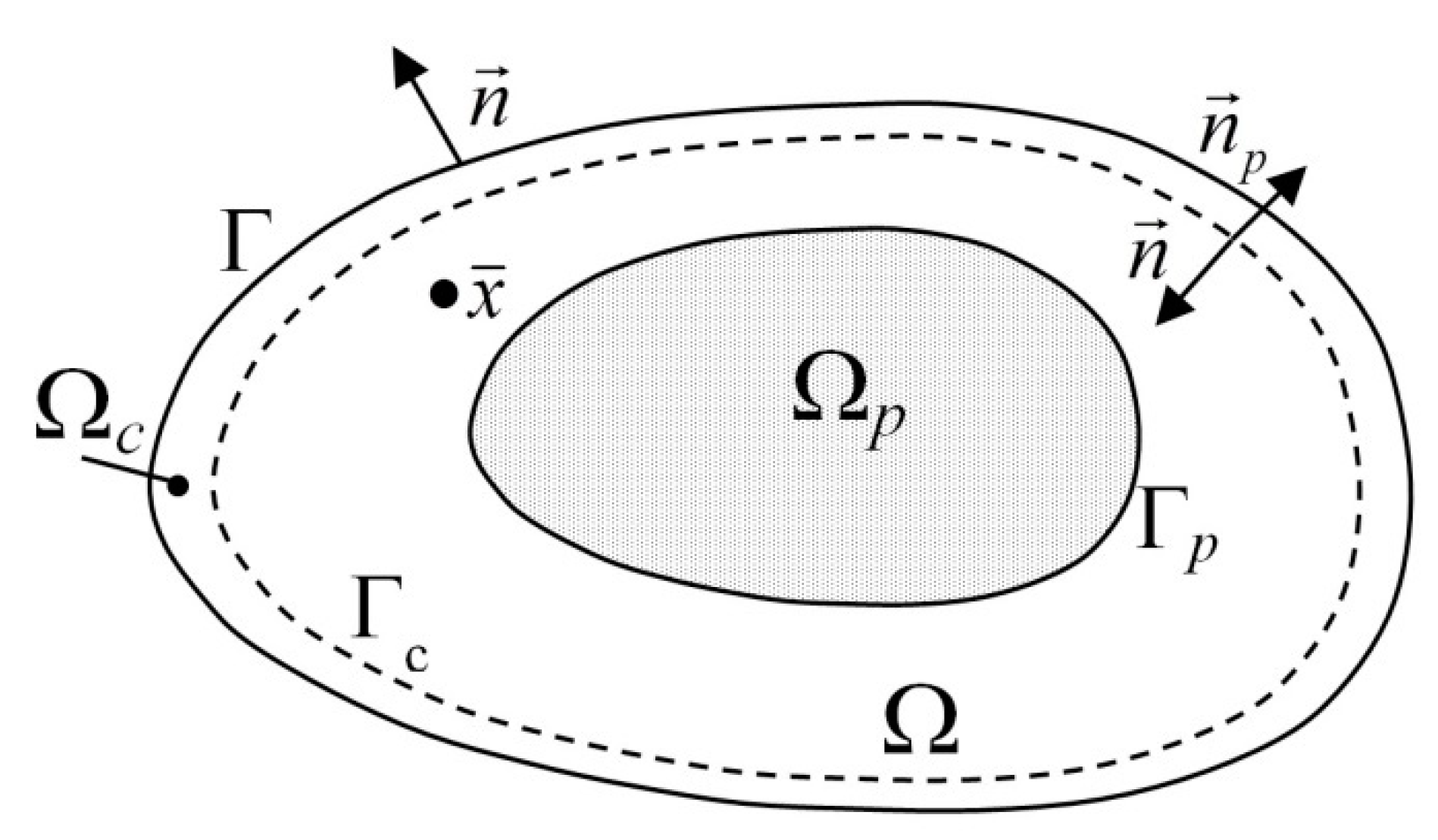
Considered is the multiply-connected domain Ω ∪ Ωc, Figure 1, divided into the region of the protective coating and the region of the blade by the boundary Γc. The problem of optimization of cooling the gas-turbine blade with a cooling channel filled with the porous material of an unknown distribution of porosity ε (0 < ε < 1), can be formulated as follows: given is the heat conduction equation in the domain Ωc ∪ Ω ∪ Ωp:
where
kc(T) is the conduction coefficient of the protective coating (ceramic), km(T) is the conduction coefficient of the material the blade is made of, kp(T,ε) is the heat conduction coefficient of the porous material, f(T, ε) is the nonzero source function in the domain Ωp
On the external boundary Γ of the domain Ωc known is the boundary condition of the third type:
where h is the heat transfer coefficient, and Tgas is the temperature of gas surrounding the area Ωc from the outside.
The distribution of porosity ε in the domain Ωp should be determined in such a way that the following condition is satisfied on the internal boundary Γc
where To is the given temperature. The unknown value of the porosity ε distribution is determined from the minimum of the functional:
In the problem under consideration, To is the constant temperature on the contact area between the material the blade is made of and the protective coating. Achieving the constant value of this temperature on the boundary Γc is possible due to filling the cooling channels properly with the porous material of the variable porosity ε.
Such posed heat conduction problem belongs to inverse problems being ill-posed in the Hadamard sense [7]. Hadamard’s definition concerns the well-posed problem, which must exist, be unique and depend continuously on the given initial conditions. If at least one of these conditions is not satisfied, the problem is ill-posed.
In direct problems being described by linear differential equations, satisfied are conditions of solution existence and uniqueness if the following conditions are satisfied:
- known is the mathematic model (differential equation describing the investigated phenomenon);
- known is the region where the investigated phenomenon occurs;
- known are physical properties in the form of coefficients resulting from the phenomenon description; such as thermal conductivity in the heat equation;
- known are forces such as heat sources;
- known are boundary and initial conditions for transient problems.
If one or more of these conditions is unknown, then the problem is an inverse one.
In such a case, additional information concerning the investigated phenomenon should be known, and the solution is sought in the least-squares sense. More details on this subject can be found in papers [8,9,10].
According to the classification given in the reference paper [11], the inverse problem considered in this paper belongs to problems related to the reproduction of the source function. Inverse problems of that type do not have an unequivocal solution [12].
Problems being solved in papers [13,14,15,16,17,18,19] concern inverse heat conduction problems related to determining unknown source function. The paper [14] has a character of the review and presents some publications relative to solving inverse problems. In papers [13,16,17], variation methods for solving inverse heat conduction problems were used, likewise in this paper. In papers [20,21,22,23,24], among others, minimization of the least-squares functional from the temperature on the surface of the region, where the boundary condition was unknown, was used to solve inverse problems.
3. Algorithm for Determining the Porosity Distribution inside the Cooling Channel of the Blade
The solution of such posed inverse problem is replaced by solving a series of direct problems for the heat Equation (1) with the third type boundary condition (4), in which the distribution of porosity ε is changing iteratively in such a way that the functional (6) achieves its minimum. An iterative algorithm is developed using variational methods. Variations of the functional and of the function are determined from the definition of the directional derivative.
The quantity ε varies inside the porous material and signifies the contribution of air to the elementary volume of the porous material [25].
Variations of Equation (1), the source function f, heat conduction coefficient k, the third type boundary condition (4) and of the functional (6) are as follows, respectively:
The variation of the functional (11) should be expressed explicitly by the variation of the variable ε. To do so, the function p conjugated to δT in the domain Ω′ = Ωc ∪ Ω ∪ Ωp is defined. From the Gauss theorem, the following identity results.
Based on (3) and (4), identity (12) takes the following form
The variation of Equation (13) is as follows
and after the Gauss theorem is applied again and the discontinuity of the normal derivative of the function p on the boundary Γc is included
hence,
and the identity (14) takes the following form
Based on (15), it can be assumed that the function p in the domain Ω′ satisfies the differential equation:
with the boundary condition:
and the discontinuity condition:
Considering the above, identity (15) takes the following form:
and the variation of the functional (11) is equal to:
and depends only on the variation of the independent variable ε.
From all possible variations of the functional (20), only those are chosen which reduce the value of the functional (6); therefore, the variation of the variable ε can be written in the form of
hence, the variation of the functional (20):
The above consideration will be next used to develop the iterative algorithm. Suppose that variables T, ε change iteratively according to the following formulae:
Knowing distributions of temperature Told and porosity εold in the previous step of the iteration, we can determine
- function u—satisfying Equation (7) in the domain Ω′ (δT = −ηu, δε = −ηv)
- Function p—satisfying Equation (16) with the boundary condition (17) and the discontinuity condition on the surface Γc (18).
Parameter η is determined from the condition that the value of the functional (6) decreases in the subsequent step of the iteration:
hence
Optimum value η is determined from the condition of the functional value maximum drop (minimum aη2 + bη):
Finally, the algorithm is as follows (see Algorithm 1)
| Algorithm 1. |
| step 1: |
| Determining the distribution of temperature T |
| while (1) |
| { |
| If abs(T − Told) > ϵT then Told = T; else break; |
| } |
| step 2: |
| Determining the distribution of the conjugate function p |
| step 3: |
| step 4: |
| Determining the distribution of the auxiliary function u |
| step 5: |
| step 6: |
| If abs(ε − εold) > ϵ then { Told = T; εold = ε; goto step 1:; } |
The algorithm is developed in such a way that in each step of the iteration, the value of the functional (6) decreases (it results from the inequality (27)). This means that the temperature on the boundary Γc approaches To, and the parameter η being determined in the fifth step of the algorithm also approaches zero. On this basis, we may assume that the condition of completing the algorithm operates in the sixth step of the algorithm is obtained with the given accuracy ϵ.
However, it does not mean that, as the result of the algorithm operation, the temperature To is achieved on the boundary Γc. It depends on the possibility of removing heat from the external boundary of the blade to the porous material. The greatest problems related to this occur in the vicinity of the blade’s trailing edge. The reference paper [6] presented some results of calculations for the algorithm developed on a basis similar to that one discussed in this paper. Inability to remove heat from this part of the blade caused the increase of temperature on the external boundary of the blade in the vicinity of the trailing edge to reduce the heat flux flowing through this region of the blade.
The algorithm considered in this paper is an expansion of the algorithm from the paper [6]. On the blade’s surface, a protective layer of a low value of the thermal conductivity coefficient was added. The desired constant value of temperature was assumed on the inner boundary, which separates the material of the blade from the protective layer. The material the blade is made of does not have contact with the external environment; therefore, the minimization functional (6) is defined on the inner boundary and not on the external boundary of the blade-like it is in the paper [6]. Application of an additional protective layer on the external boundary of the blade results in solving different differential equations in each step of the iteration than it is in the case of the algorithm discussed in paper [6].
4. Determining the Distribution of Porosity in Cooling Channels of the Gas Turbine Blades Coated with a Protective Layer
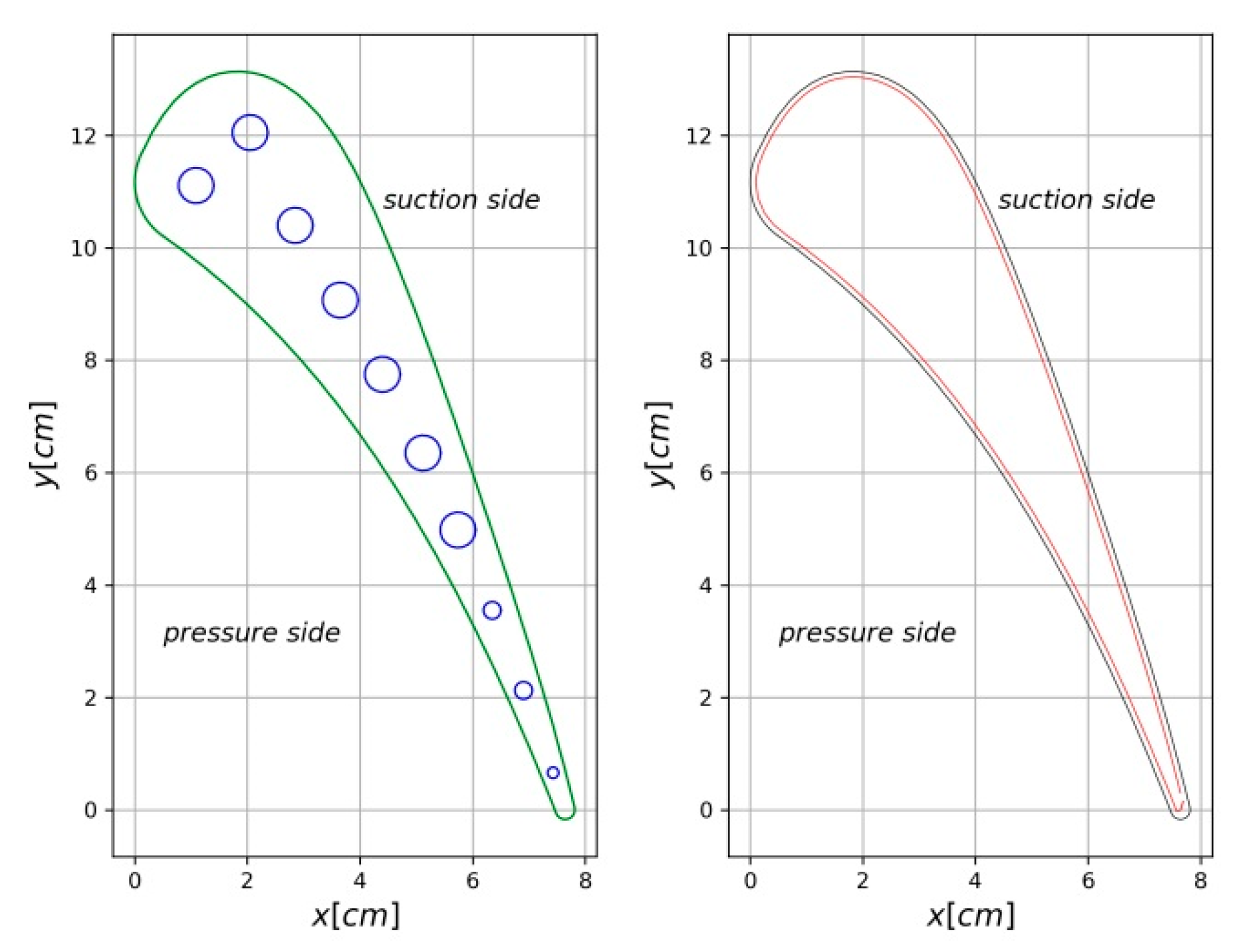
The blade-shaped, as shown in Figure 2 (right), with one cooling channel filled with a porous material, was chosen for numerical calculations. The external surface of the blade was coated with the protective layer being thick, as summarized in Table 1. The source function is related to the porous material and is given by the following formula [25]:
where Tair denotes the temperature of the air flowing through the porous material, and hV is the volumetric heat transfer coefficient determined from the formula:
In the formula (30), U denotes the velocity of air flowing through the porous material [m/s], dp—the pore diameter [mm], C, x, y, z are nondimensional coefficients determined based on experimental research [25], summarized in Table 2.
Heat conduction coefficients for the material of the blade’s protective layer and for the porous material are given by the formula
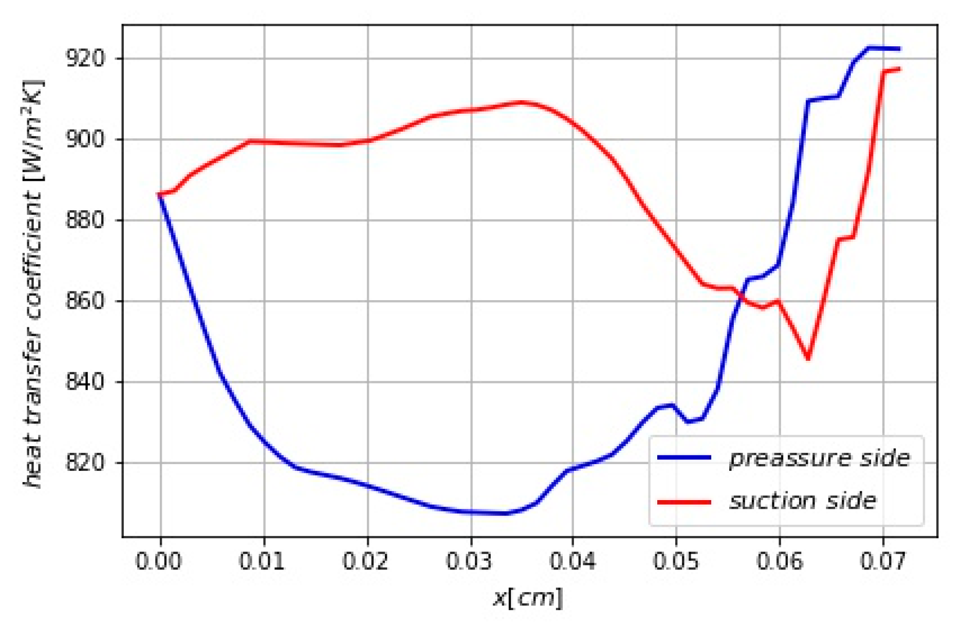
The heat transfer coefficient on the external boundary of the blade was adopted from the research results included in the reference paper [26], and its distribution is shown in Figure 3. The temperature of gas surrounding the blade Tgas equals 800 K, and the temperature of the air cooling the Tair equals 300 K. Calculations were performed for temperature To on the boundary Γc of 550, 600, 650 K, respectively.
Differential equations in subsequent steps of the algorithm from Section 2 were solved using the finite element method included in the FreeFem++ software [27]. For numerical calculations, a mesh of finite elements consisting of 26,338 triangle elements was used. Calculations were performed by approximating the solution in the mesh element with the use of Lagrangian finite elements P1 and P2, and they gave identical solutions. Equations from subsequent steps of the algorithm were of the following form:
- Step 1:
- Step 2:
- Step 3:
Calculations were performed for thicknesses of the protective coating given in Table 1. Thickness was diversified maximally to show its impact on the efficiency of heat removal through the porous material placed inside the blade’s cooling channel.
To evaluate the deviation of the temperature distribution on the boundary between the protective layer and the material the blade is made of the following norm was used:
where lΓc is the length of the boundary Γc.
Results of calculations performed for the protective coating of a thickness of g = 30 μm are presented in Figure 4, Figure 5, Figure 6 and Figure 7.
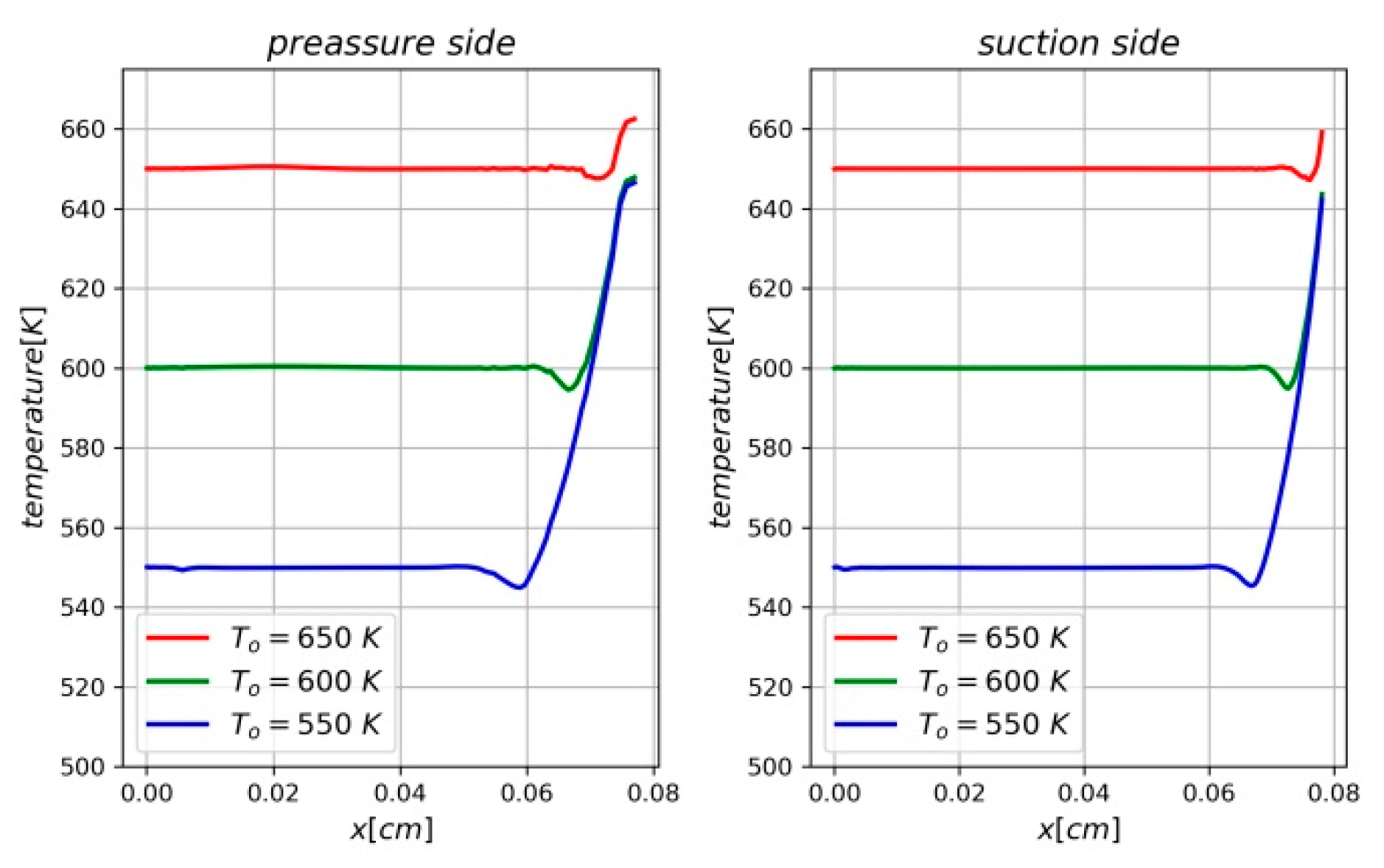
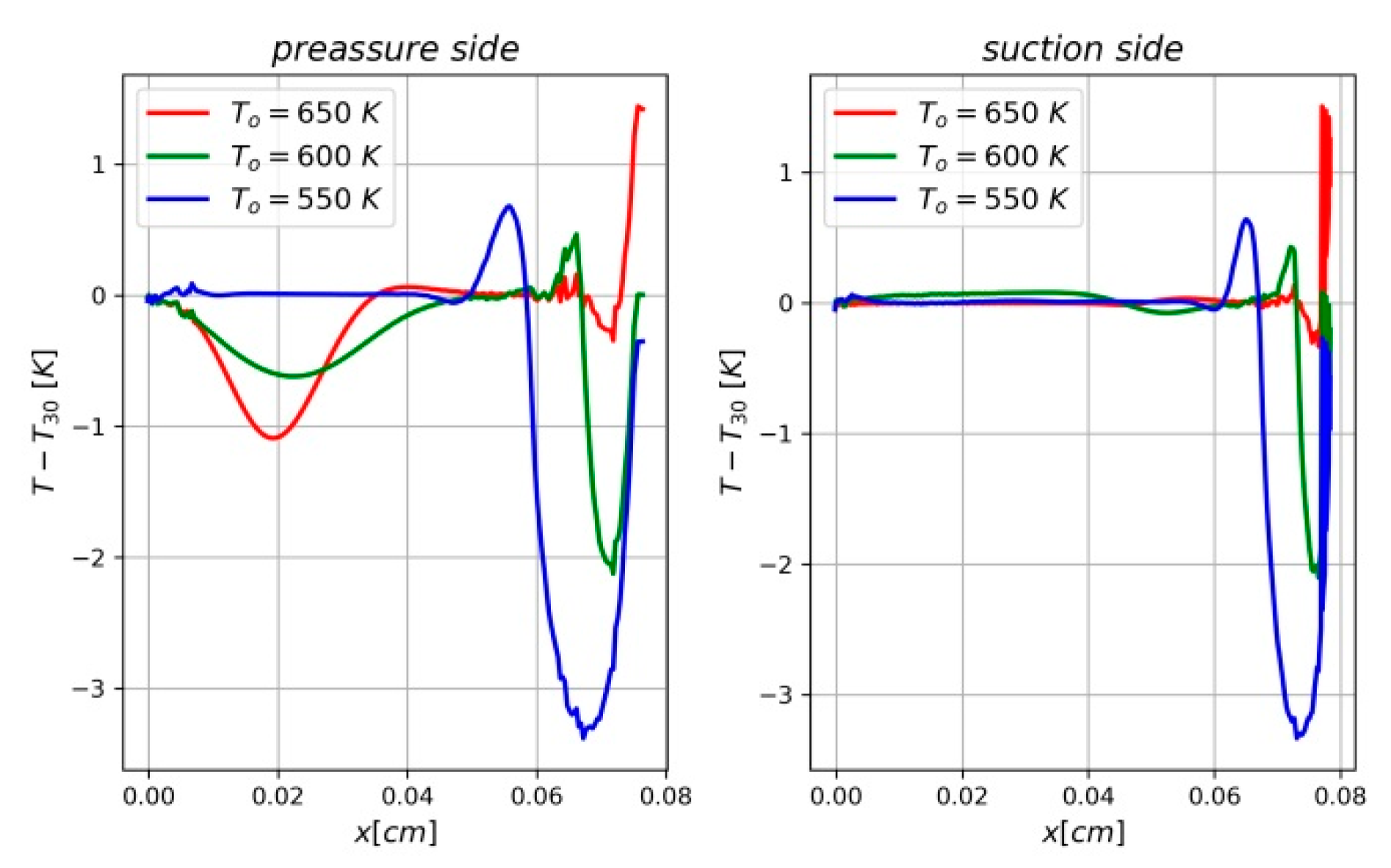
Figure 4 presents the distribution of temperature on the boundary between the protective coating and the blade’s surface for the protective coating being 30 μm-thick. This distribution was approximated in the iteration process to the temperature To given on the contact area between the protective coating and the material the blade is made of. When compared with the assumed value of temperature To, the greatest differences occur in the vicinity of the trailing edge, both, on the suction side and on the pressure side of the blade. The region where these differences occur widens while the value of temperature To decreases.
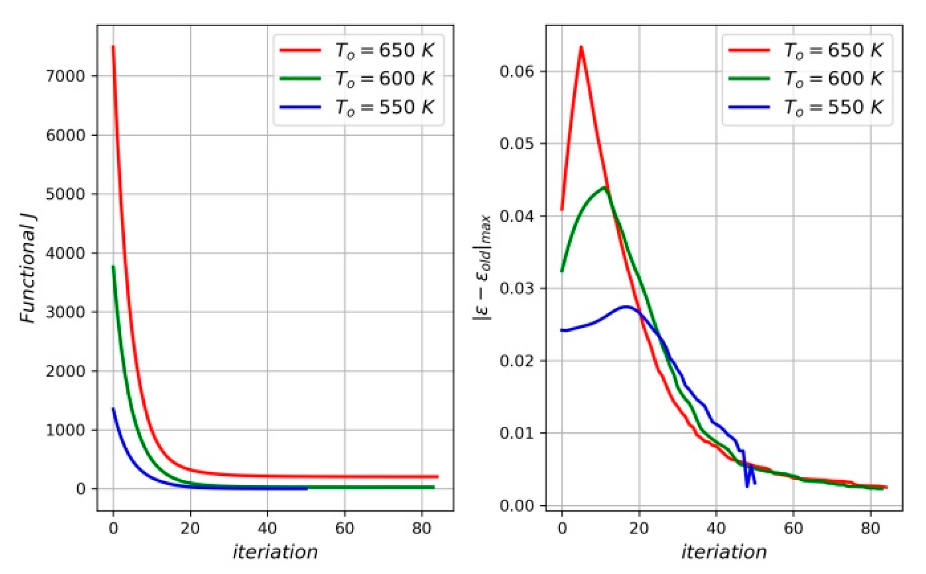
The accuracy of the algorithm operation for the protective coating thickness of 30 μm is presented in Figure 5 (left). It is noticeable that in subsequent steps of iteration, the value of the functional (6) decreases. The same figure (right) shows the course of the distribution of the maximum value of the porosity difference |ε − εold|max in subsequent steps of iteration. The algorithm completes its operation when the value of this difference drops below 0.002.
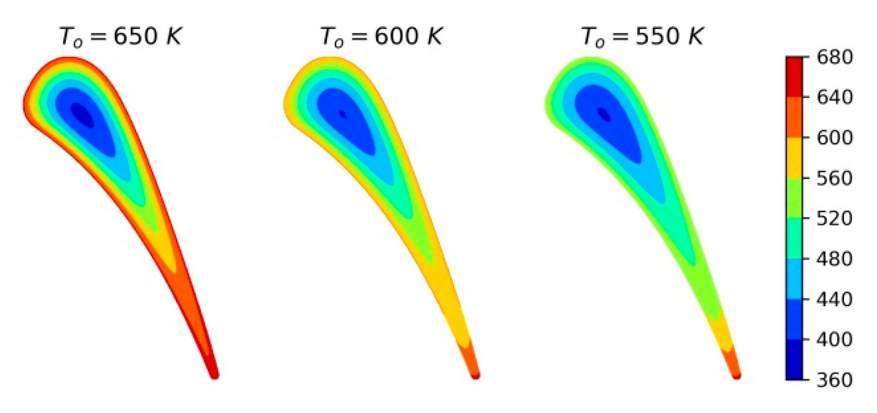
Figure 6 presents the distribution of temperature in the entire area of the blade without the protective coating. The increase of the blade’s temperature in the vicinity of the trailing edge is clearly noticeable.
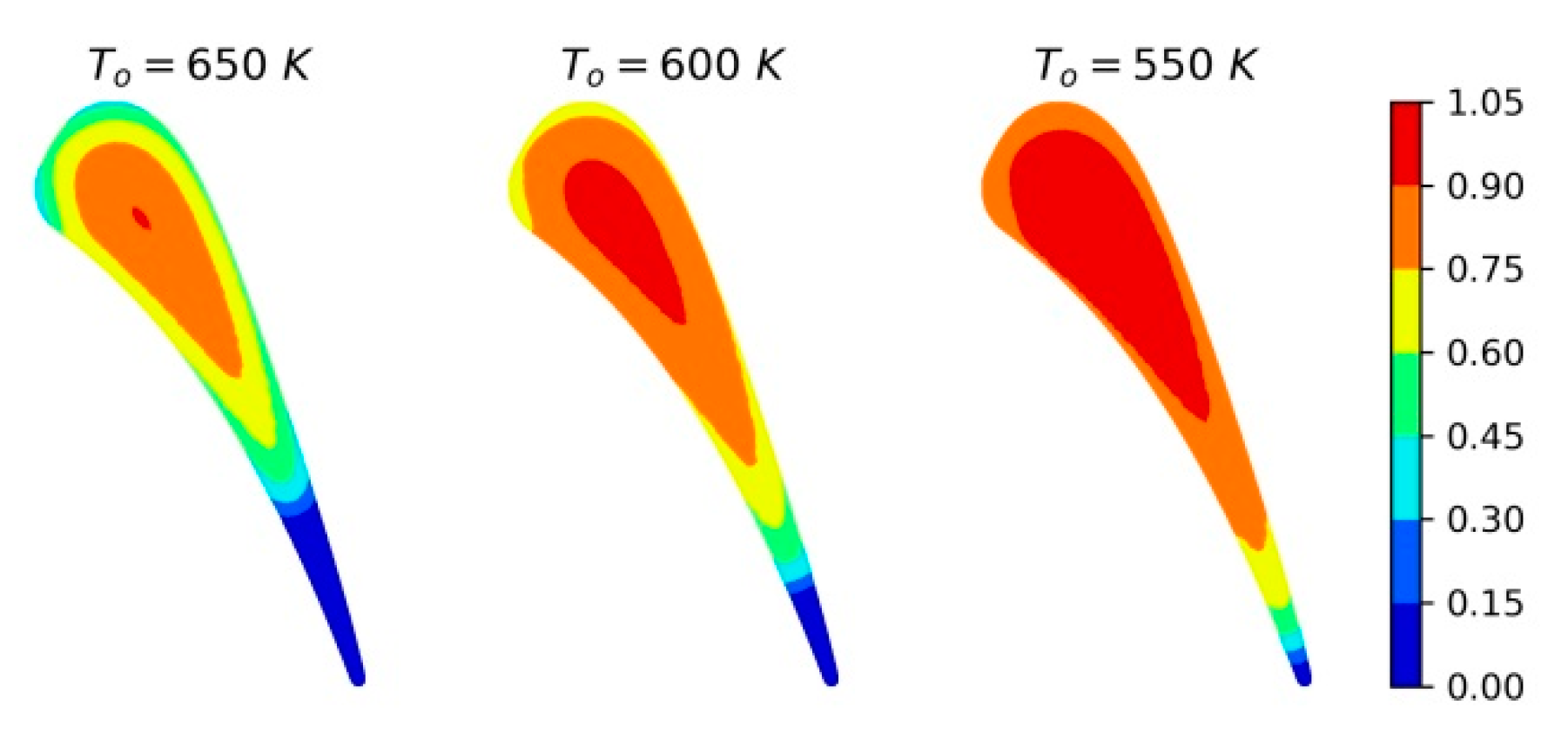
Distribution of the porous material, determined with the use of the algorithm discussed in Section 2, for the protective coating being 30 μm-thick, is shown in Figure 7. Value 1 denotes only air, and value 0 denotes only material the blade is made of. The volumetric heat transfer coefficient hV (30) increases while the porosity decreases. This is obvious, since with the increase of the air quantity in the porous material volume unit, its involvement in conducting heat through the porous material to the internal part of the channel decreases.
The formula (30) cannot, however, be extrapolated for ε = 0, since this is the borderline case when the porous material becomes the material of a continuous structure. According to the formula (30), this coefficient has the highest value, although it does not remove the accumulated heat. It is similar to the borderline case ε = 1 when the volumetric heat transfer coefficient should approach the surface heat transfer coefficient. As properties of the porous material do not behave on the boundary in such a way, minimum and maximum values of porosity of 0.05 and 0.95, respectively, were assumed for calculations.
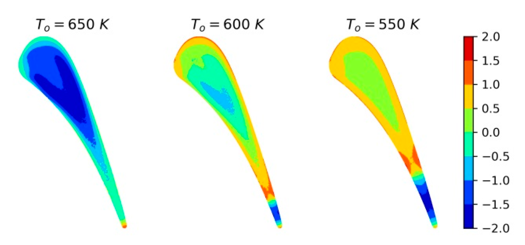
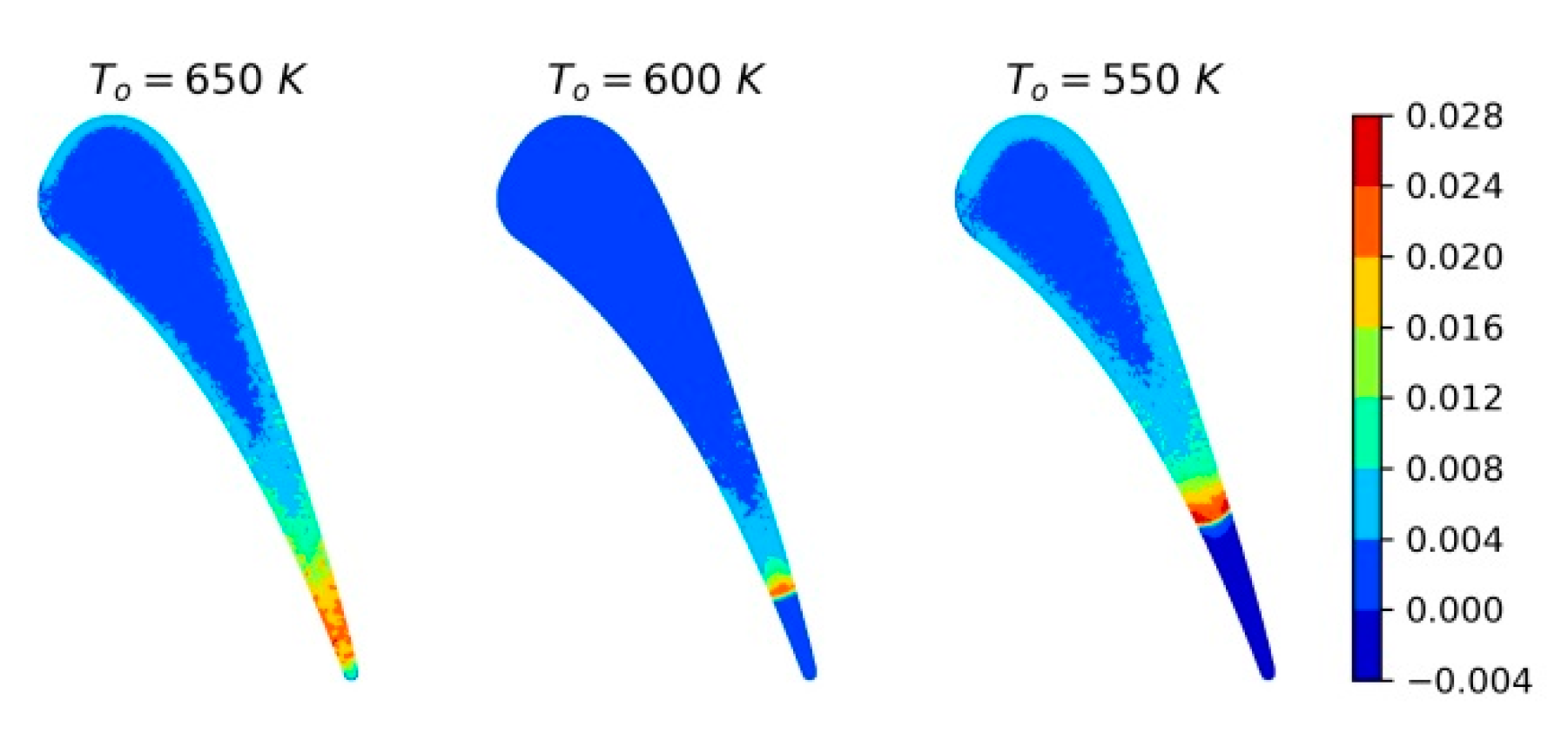
Results of calculations for the protective layer being 200 μm thick are presented in Figure 8, Figure 9 and Figure 10. Due to a great similarity between distributions of temperature and of porosity for this thickness to distributions shown in Figure 4, Figure 6 and Figure 7, these figures present the difference between distributions of temperature and of porosity for the thicker layer and distributions for the protective layer being 30 μm thick.
The distribution of the temperature difference on the contact surface between the protective layer and the blade is the greatest in the vicinity of the trailing edge, and it coincides with the region where the greatest difference of the temperature calculated by the algorithm relative to the temperature To occurs.
This difference is more visible in Figure 9 for the temperature distribution and in Figure 10 for the porosity distribution in the entire blade.
The increase of the protective layer thickness did not significantly improve conditions of heat exchange in the vicinity of the blade’s trailing edge. This can be interpreted as follows: the protective layer allows for limiting the heat flow into the blade’s interior to enable removing heat by convection and by conduction through the porous material placed inside the cooling channel. Due to the thickness of the same blade in the region close to the trailing edge, it is impossible to transfer such an amount of heat to the porous material to achieve a temperature approximately equal to. Only for To = 650 K this was possible.
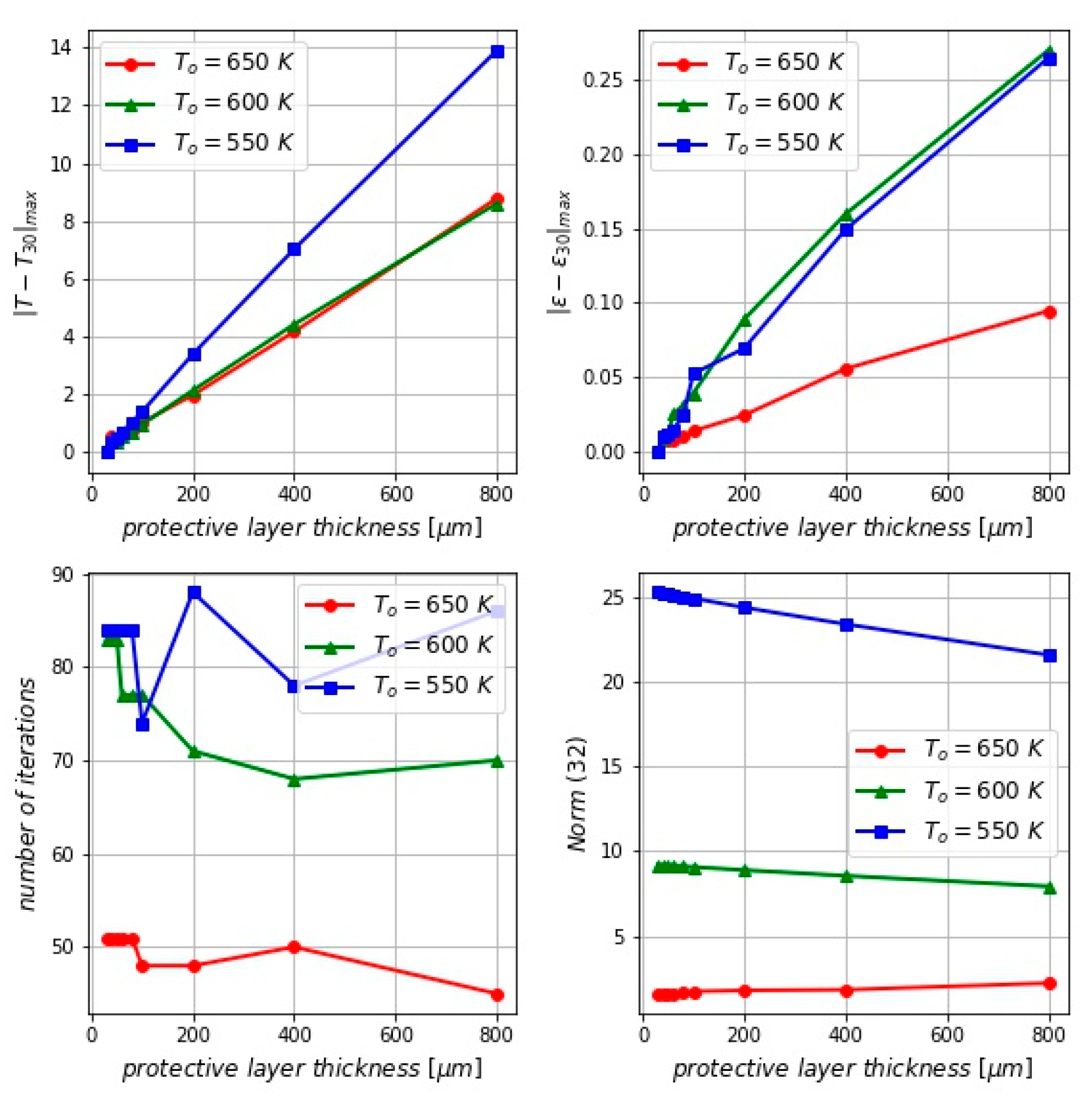
The synthetic presentation of selected quantities in the function of the protective layer thickness given in Table 1 is shown in Figure 11.
For various thicknesses of the protective layer, similar distributions of temperature in the blade were obtained. The maximum temperature difference did not exceed 14 K, Figure 11 (top, left). Significant differences, reaching 25% of maximum porosity value, were observed for the porosity distribution, Figure 11 (top, right). The region of the blade where the highest differences occurred was at the place where the blade’s throat begun towards the trailing edge, Figure 10. The number of iterations needed to perform calculations is shown in Figure 11 (bottom, left). An increase of the coating layer thickness does not impact significantly on the temperature distribution on the contact area between the protective surface and the blade, Figure 11 (bottom, right).
5. Conclusions
The performed calculations indicate that it is possible to effectively remove heat from the interior of the blade due to the application of the protective layer on the blade’s surface. Calculations were performed with the use of the algorithm allowing for such determining the porosity distribution that the given temperature To is achieved at the contact area between the external surface of the blade and the protective layer. Results of calculations and their interpretation are presented in the previous section.
Research tests prove that the efficiency of the blade’s protection against high-temperature impact and the satisfaction of the optimization criterion demand synchronization of both protection methods, that is, the application of a protective layer with cooling the blade using the porous material. However, even this is not enough to achieve a rather stable value of temperature on the contact surface between the protective layer and the material the blade is made of. This is caused by the difficulty of removing heat from the region close to the trailing edge.
Performed calculations also indicate that the increase of the blade’s protective layer thickness does not improve the conditions of heat exchange.
Calculations were made for a chosen blade profile. However, the algorithm presented in this paper is not limited to such a choice and can be used for calculations performed in three dimensions.
Author Contributions
Conceptualization, A.F.; methodology, A.F. and A.O.; software, A.F.; validation, A.W. and M.C.; formal analysis, A.F. and. M.C.; investigation, A.W.; resources, A.O.; data curation, A.F. and. A.W.; writing—original draft preparation, A.F. and. A.W.; writing—review and editing, M.C.; visualization, A.W.; supervision, A.F. and. A.O. All authors have read and agreed to the published version of the manuscript.
Funding
This research was funded by Politechnika Poznańska.
Institutional Review Board Statement
Not applicable.
Informed Consent Statement
Not applicable.
Data Availability Statement
Data sharing not applicable.
Conflicts of Interest
The authors declare no conflict of interest.
References
- Lakshminarayana, B. Fluid Dynamics and Heat Transfer of Turbomachinery; John Wiley & Sons: Hoboken, NJ, USA, 1996. [Google Scholar]
- Bunker, R.S. Gas Turbine Heat Transfer. 10 Remaining Hot Gas Path Challenges. J. Turbomach. 2007, 129, 193–201. [Google Scholar] [CrossRef]
- Brenberg, J. Turbulence Modelling for Internal Cooling of Gas-Turbine Blades. Ph.D. Thesis, Department of Thermo and Fluid Dynamics, Chalmers University of Technology, Goeteborg, Sweden, 2002. [Google Scholar]
- Beck, T.; Klopf, J. Verfahren zur Herstellung einer innengekühlten Turbinenschaufel und Gasturbine mit einer so hergestellten Turbinenschaufel. European Patent EP 2418354A1, 21 November 2001. [Google Scholar]
- Aubert, J.-P.; Tirol, J. Process for the manufacture of turbine blades cooled and product obtained by the process. United States Patent 4 400 834, 3 April 1984. [Google Scholar]
- Frąckowiak, A.; von Wolfersdorf, J.; Ciałkowski, M. Optimization of cooling of gas turbine blades with channels filled with porous material. Int. J. Therm. Sci. 2019, 136, 370–378. [Google Scholar] [CrossRef]
- Hadamard, J. Sur les problèmes aux dérivéespartielles et leur signification physique. Princet. Univ. Bull. 1902, 13, 49–52. [Google Scholar]
- Alifanov, O.M. Inverse Heat Transfer Problems; Springer: Berlin, Germany, 1994. [Google Scholar]
- Beck, J.V.; Blackwell, B.; Clair, C.R. Inverse Heat Conduction: Ill-Posed Problems; John Wiley and Sons, Inc.: New York, NY, USA, 1985. [Google Scholar]
- Louis, A.K. Inverse und Schlecht Gestellte Probleme; Teubner Studienbücher Mathematik: Stuttgart, Germany, 1989. [Google Scholar]
- Dulikravich, G.S.; Martin, T.J.; Dennis, B.H. Multidisciplinary inverse problems. In Proceedings of the 3rd International Conference on Inverse Problems in Engineering (3icipe): Theory and Practice, Port Ludlow, WA, USA, 13–18 June 1999. [Google Scholar]
- Alves, C.J.S.; Colaço, M.J.; Leitão, V.M.A.; Martins, N.F.M.; Orlande, H.R.B.; Roberty, N.C. Recovering the source term in a linear diffusion problem by the method of fundamental solutions. Inverse Probl. Sci. Eng. 2010, 16, 1005–1021. [Google Scholar] [CrossRef]
- Frąckowiak, A.; Botkin, N.D.; Ciałkowski, M.; Hoffmann, K.-H. Iterative algorithm for solving the inverse heat conduction problems with the unknown source function. Inverse Probl. Sci. Eng. 2015, 23, 1056–1071. [Google Scholar] [CrossRef]
- Mierzwiczak, M.; Kołodziej, J.A. The determination of heat sources in two dimensional inverse steady heat problems by means of the method of fundamental solutions. Inverse Probl. Sci. Eng. 2011, 19, 777–792. [Google Scholar] [CrossRef]
- Yan, L.; Fu, C.-L.; Yang, F.-L. The method of fundamental solutions for the inverse heat source problem. Eng. Anal. Boundary Elem. 2008, 32, 216–222. [Google Scholar] [CrossRef]
- Johansson, T.; Lesnic, D. A variational method for identifying a spacewise-dependent heat source. IMA J. Appl. Math. 2007, 72, 748–760. [Google Scholar] [CrossRef]
- Geng, F.; Lin, Y. Application of the variational iteration method to inverse heat source problems. Comp. Math. Appl. 2009, 58, 2098–2102. [Google Scholar] [CrossRef] [Green Version]
- Ling, L.; Yamamoto, M.; Hon, Y.C.; Takeuchi, T. Identification of source locations in two-dimensional heat equations. Inverse Probl. 2006, 22, 1289–1305. [Google Scholar] [CrossRef]
- Yang, C.-Y. The determination of two heat source in an inverse heat conduction problem. Int. J. Heat Mass Transf. 1999, 42, 345–356. [Google Scholar] [CrossRef]
- Frąckowiak, A.; von Wolfersdorf, J.; Ciałkowski, M. An iterative algorithm for the stable solution of inverse heat conduction problems in multiply-connected domains. Int. J. Therm. Sci. 2015, 96, 268–276. [Google Scholar] [CrossRef]
- Joachimiak, M.; Ciałkowski, M.; Frąckowiak, A. Stable method for solving the Cauchy problem with the use of Chebyshev polynomials. Int. J. Numer. Methods Heat Fluid Flow 2019, 30, 1441–1456. [Google Scholar] [CrossRef]
- Ciałkowski, M.; Olejnik, A.; Frąckowiak, A.; Lewandowska, N.; Mosiężny, J. Cauchy type inverse problem in a two-layer area in the blades of gas turbine. Energy 2020, 212, 118751. [Google Scholar] [CrossRef]
- Grysa, K.; Maciag, A.; Pawińska, A. Solving nonlinear direct and inverse problems of stationary heat transfer by using Trefftz functions. Int. J. Heat Mass Transf. 2012, 55, 7336–7340. [Google Scholar] [CrossRef]
- Maciąg, A. The usage of the Trefftz method to determine the Biot number. J. Appl. Math. Comput. Mech. 2017, 16, 47–55. [Google Scholar] [CrossRef] [Green Version]
- Fuller, A.J.; Kim, T.; Hodson, H.P.; Lu, T.J. Measurement and interpretation of the heat transfer coefficients of metal foams. Proc. Inst. Mech. Eng. Part C J. Mech. Eng. Sci. 2005, 219, 183–191. [Google Scholar] [CrossRef]
- Hylton, L.D.; Mihelc, M.S.; Turner, E.R.; Nealy, D.A.; York, R.E. Analytical and Experimental Evaluation of the Heat Transfer Distribution over the Surfaces of Turbine Vanes; Final Report Detroit Diesel Allison, Tech. Rep.; NASA: Washington, DC, USA, 1983.
- Hecht, F. FreeFem++. Available online: http://www.freefem.org/ff++ (accessed on 1 May 2014).
Figure 1.
Domain Ω surrounded by the external layer of the protective coating Ωc, filled inside with the porous material Ωp.
Figure 1.
Domain Ω surrounded by the external layer of the protective coating Ωc, filled inside with the porous material Ωp.

Figure 2.
Blade C3x of the gas turbine with ten cooling channels (left) and the blade coated with the protective layer on the external surface (right).
Figure 2.
Blade C3x of the gas turbine with ten cooling channels (left) and the blade coated with the protective layer on the external surface (right).

Figure 3.
Distribution of the heat transfer coefficient on the blade’s external boundary.

Figure 4.
Distributions of temperature on the boundary between the protective layer and the material the blade is made of for the protective coating thickness of 30 μm.
Figure 4.
Distributions of temperature on the boundary between the protective layer and the material the blade is made of for the protective coating thickness of 30 μm.

Figure 5.
The course of the functional J [ε] (6) in subsequent iterations of the algorithm (left); the course of the maximum change in porosity distribution (right) in subsequent iterations of the algorithm, protective coating thickness g = 30 μm.
Figure 5.
The course of the functional J [ε] (6) in subsequent iterations of the algorithm (left); the course of the maximum change in porosity distribution (right) in subsequent iterations of the algorithm, protective coating thickness g = 30 μm.

Figure 6.
Distribution of temperature inside the blade; protective coating thickness g = 30 μm.

Figure 7.
Distribution of porosity ε in the porous material; protective coating thickness g = 30 μm.
Figure 7.
Distribution of porosity ε in the porous material; protective coating thickness g = 30 μm.

Figure 8.
Distributions of the difference between temperatures on the boundary between the protective layer and the material the blade is made of for g = 200 μm and g = 30 μm.
Figure 8.
Distributions of the difference between temperatures on the boundary between the protective layer and the material the blade is made of for g = 200 μm and g = 30 μm.

Figure 9.
Distributions of temperature difference for g = 200 μm and g = 30 μm.

Figure 10.
Distributions of porosity ε difference for g = 200 μm and g = 30 μm.

Figure 11.
Distributions of selected quantities in the function of the protective coating thickness.
Figure 11.
Distributions of selected quantities in the function of the protective coating thickness.


Table 1.
Thickness of the protective layer (μm).
| g | 30 | 40 | 50 | 60 | 80 | 100 | 200 | 400 | 800 |
Table 2.
Numerical values for the coefficients in Equation (30), [25].
Table 2.
Numerical values for the coefficients in Equation (30), [25].
| C (-) | U (m/s) | dp (mm) | x (-) | y (-) | z (-) |
|---|---|---|---|---|---|
| 356,300 | 5 | 2 | 0.954 | 0.51 | 0.46 |
Publisher’s Note: MDPI stays neutral with regard to jurisdictional claims in published maps and institutional affiliations. |
© 2020 by the authors. Licensee MDPI, Basel, Switzerland. This article is an open access article distributed under the terms and conditions of the Creative Commons Attribution (CC BY) license (http://creativecommons.org/licenses/by/4.0/).
Share and Cite
MDPI and ACS Style
Frąckowiak, A.; Olejnik, A.; Wróblewska, A.; Ciałkowski, M. Application of the Protective Coating for Blade’s Thermal Protection. Energies 2021, 14, 50. https://doi.org/10.3390/en14010050
AMA Style
Frąckowiak A, Olejnik A, Wróblewska A, Ciałkowski M. Application of the Protective Coating for Blade’s Thermal Protection. Energies. 2021; 14(1):50. https://doi.org/10.3390/en14010050
Chicago/Turabian StyleFrąckowiak, Andrzej, Aleksander Olejnik, Agnieszka Wróblewska, and Michał Ciałkowski. 2021. "Application of the Protective Coating for Blade’s Thermal Protection" Energies 14, no. 1: 50. https://doi.org/10.3390/en14010050
Note that from the first issue of 2016, this journal uses article numbers instead of page numbers. See further details here.