Development of Simulation Tool for Ground Source Heat Pump Systems Influenced by Ground Surface


1
Faculty of Engineering, Hokkaido University, N13-W8, Kita-ku, Sapporo 060-8628, Japan
2
Graduate School of Engineering, Hokkaido University, N13-W8, Kita-ku, Sapporo 060-8628, Japan
*
Author to whom correspondence should be addressed.
Energies 2020, 13(17), 4491; https://doi.org/10.3390/en13174491
Submission received: 25 May 2020
/
Revised: 9 August 2020
/
Accepted: 21 August 2020
/
Published: 31 August 2020
(This article belongs to the Special Issue Ground Source Heat Pumps as Efficient and Sustainable Systems in Buildings)
Abstract
:The authors developed a ground heat exchanger (GHE) calculation model influenced by the ground surface by applying the superposition theorem. Furthermore, a simulation tool for ground source heat pump (GSHP) systems affected by ground surface was developed by combining the GHE calculation model with the simulation tool for GSHP systems that the authors previously developed. In this paper, the outlines of GHE calculation model is explained. Next, in order to validate the calculation precision of the tool, a thermal response test (TRT) was carried out using a borehole GHE with a length of 30 m and the outlet temperature of the GHE calculated using the tool was compared to the measured one. The relative error between the temperatures of the heat carrier fluid in the GHE obtained by measurement and calculation was 3.3% and this result indicated that the tool can reproduce the measurement with acceptable precision. In addition, the authors assumed that the GSHP system was installed in residential houses and predicted the performances of GSHP systems using the GHEs with different lengths and numbers, but the same total length. The result showed that the average surface temperature of GHE with a length of 10 m becomes approximately 2 °C higher than the average surface temperature of a GHE with a length of 100 m in August.
1. Introduction
In the recent years, global warming due to increase of CO2 emission has become a worldwide environmental issue. Therefore, ground source heat pump (GSHP) systems, which use the underground thermal energy as a heat sink/source and supply cooling, heating, and/or hot water with high efficiency, have attracted widespread attention. Several million units have been installed in the world [1]. However, the number of GSHP system installed in Japan is still low although it is gradually increasing. The main reason is that the installation cost of ground heat exchangers (GHEs) is expensive due to the complex underground formations. The utilization of shallow underground thermal energy such as short GHEs, energy piles and horizontal GHEs is effective to reduce the installation cost especially for the small building.
Recently, several research reports related to the use of short GHEs have been provided. A short vertical ground heat exchanger with a borehole length of 3 m and a helical shaped pipe was evaluated by means of a network of interconnected thermal resistance and capacitance [2]. Zarrella et al. analyzed short helical and double U-tube borehole heat exchangers and concluded that the helical heat exchanger had better performance than the double U-tube [3]. The operation modes of GSHP systems with short helical GHEs were also investigated [4]. Furthermore, there are several research reports on the use of piles. Hamada et al. evaluated the performance of energy piles installed in a building [5]. The authors have reported heating tests of GSHP systems using steel pipe foundation piles as GHEs in cold regions [6] and the effectiveness of using foundation piles in residential houses in moderate climate regions using simulations [6]. Furthermore, a simulation of a GSHP system using energy piles with short lengths and a large diameter was introduced [7]. With regard to research on horizontal GHEs, Fujii et al. developed a numerical model for slinky-coil horizontal GHEs and evaluated the performance [8,9]. Li et al. developed a simulation model for horizontal slinky GHEs by applying the analytical solution of ring source [10,11]. Xiong et al. developed a response function (g-function) for horizontal slinky GHEs [12].
Regarding the utilization of shallow ground thermal energy, the performance of GHEs may decrease due to the influence of the ambient air temperature and solar radiation. In a heating test using steel pipe foundation piles as a GHE actually performed in the cold district mentioned above [6], no building was constructed above the GHE, and the ground surface was in contact directly with the ambient air. As a result, the decrease of ground temperature become larger than the decrease calculated using the simulation. From this, it is necessary to predict the performance of GHEs affected by the ambient air temperature and the solar radiation on the ground surface. The ground temperature considering the influence of the ambient air temperature and solar radiation can be obtained by applying a numerical analysis [13] or an analytical solution of semi-infinite solid, surface temperature periodic with time [14]. For the latter (applying the analytical solution of semi-infinite solid), it is possible to superpose it with the ground temperature variation caused by the heat injection/extraction via GHEs, which is calculated by applying the analytical solution of line source or cylindrical heat source. Bandos et al. calculated the ground temperature variation in a thermal response test considering the influence of ground surface temperature by superposing the analytical solutions of finite line source and semi-infinite solid, surface temperature periodic with time [15].
In this study, the authors applied the superposition theorem and considered the influence of the ground surface on the GHE calculation model, which can be applied for a short GHE and a horizontal GHE. Then, a simulation tool for a GSHP system influenced by the ground surface was developed by combining the GHE calculation model with the simulation tool that the authors developed [6,7,16,17]. The outlines of the calculation model for a short GHE is firstly explained (the calculation model for a horizontal GHE will be introduced in the future). Next, a thermal response test (TRT) was carried out using a borehole GHE with a length of 30 m, and the outlet temperature of the GHE was calculated using the developed tool and compared with the measured one. In addition, the authors assumed that a GSHP systems using GHEs of different numbers and different lengths, but the same total length, was installed in residential houses and evaluated the performance using a simulation tool.
2. Calculation Model for Ground Source Heat Pump Systems Influenced by Ground Surface
2.1. Overview of Ground Temperature Calculation
Soil is treated as an infinite isotonic constant solid, and the ground surface is considered as a flat solid surface without water evaporation and condensation. Then, the heat transfer in the ground surrounding the GHE can be treated as an axisymmetric three-dimensional unsteady heat transfer problem in a cylindrical coordinate system, and it is expressed as Equation (1).
Here, the initial condition is set as , and the boundary condition is set as . By applying the superposition theorem, the temperature variation in the ground surrounding the GHE caused by the influence of the ground surface and the heat injection/extraction via the GHEs can be calculated as in Equation (2) [15].
Here, the gradient of ground temperature is not considered because the authors targeting GHEs up to about 100 m in depth. However, if the deep boreholes with several hundred meters are targeted, it is required to consider the gradient of ground temperature [18]. This challenge will be addressed in the future. Where, the first term on the right side is the initial temperature. The second term is the temperature variation caused by the heat injection/extraction via the GHEs, and the initial condition is set as and the boundary condition is set as . If the heat injection rate via the GHE is constant, can be calculated by using the analytical solution of finite line source. The equation can be expressed as the following [19].
Here,
The third term is the temperature variation affected by the influence of the ground surface, and the initial condition is set as and the boundary condition is set as . Here, is the equivalent ambient air temperature and is calculated using Equation (4) [20].
Here, the first term on the right side is the ambient temperature, the second term and the third term are temperature variations affected by the solar radiation and the effective radiation, respectively. The effective radiation is obtained as the difference between the downward atmospheric radiation to the ground surface and the upward ground surface radiation to the atmosphere. In order to calculate the underground temperature distribution, the equivalent ambient air temperature is approximated to a periodic function by harmonic analysis of monthly temperature and solar radiation at an arbitrary point [20]. The monthly temperature and solar radiation can be obtained from the extended AMeDAS weather data [21]. Then, the underground temperature considering the influence of ground surface can be calculated using Equation (5) [20].
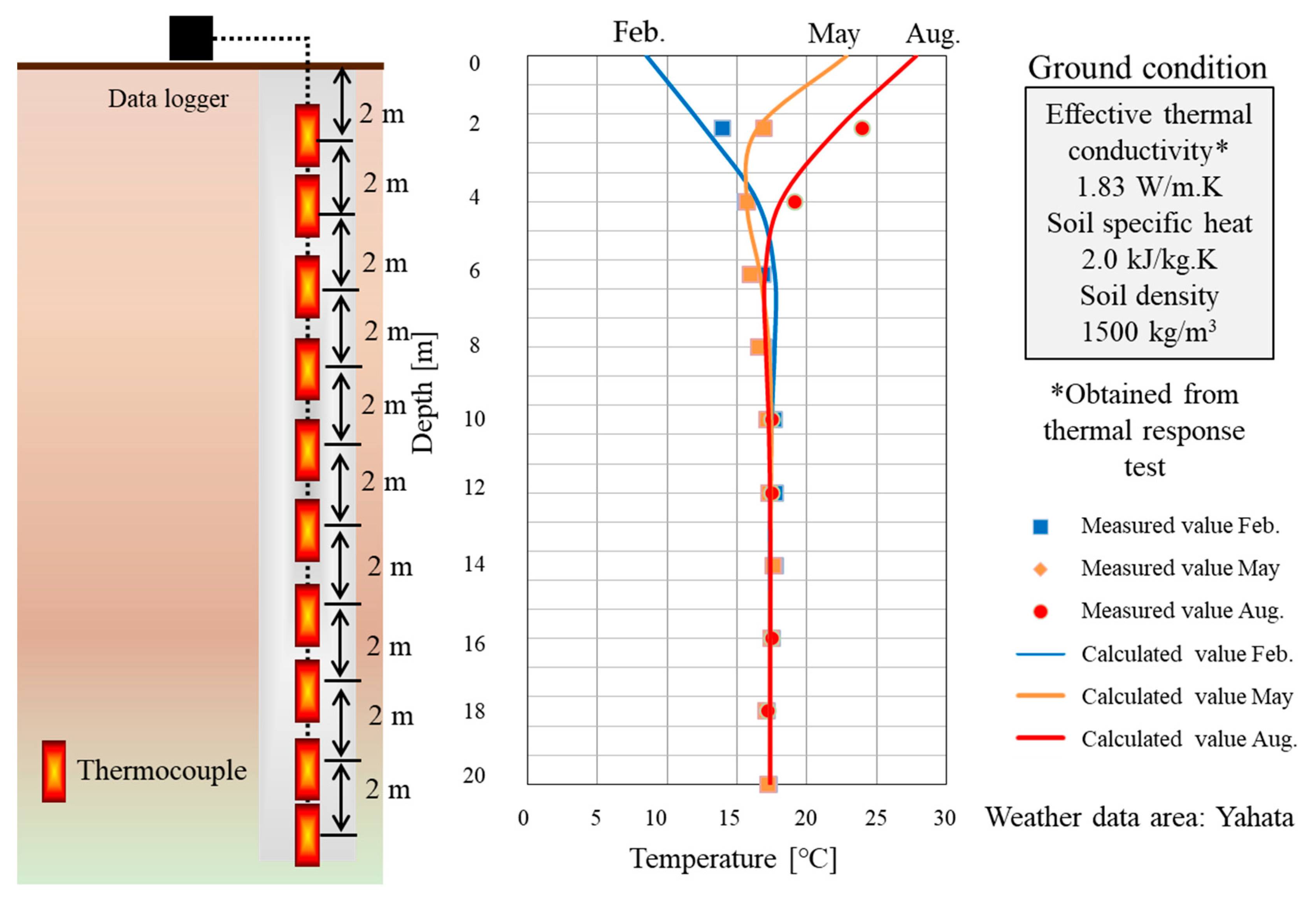
where is the ground temperature affected by the ambient air temperature variation, is the temperature variation affected by the solar radiation and is the temperature affected by the effective radiation. For example, according to the extended AMeDAS weather data of Yahata (Kitakyushu), the outdoor temperature and solar radiation values for a standard year can be obtained, therefore, and can be approximated to Equations (6) and (7).
The calculated results are compared with the measured data. The 20 m borehole used in this experiment is installed on the campus of The University of Kitakyushu (Kitakyushu city, Japan). The schematic diagram and comparison results are shown in Figure 1. Here, is given as [19]. Figure 1 compares the temperature distributions in different months (February, May and August) and at different depths. The calculation result shows the acceptable precision. Therefore, it can be determined that is used for simulation.
2.2. Overview of Ground Temperature Calculation in Simulation Tool
The average surface temperature of the GHE, , can be obtained using Equation (8).
The second term on the right side is a temperature variation affected by the heat injection/extraction via GHEs. Here, the initial condition is and the boundary condition is . The average surface temperature variation can be obtained using Equation (9), which can consider multiple GHEs [7].
where the subscript indicates the GHE under consideration, indicates a neighboring GHE, and . Thus, the first term on the right side means the average temperature variation due to the heat injection/extraction via the GHE under consideration and the second term is the average temperature variation due to the heat injection/extraction via the neighboring GHEs. Applying the superposition in the time of the ICS solution is the most suitable to calculate the surface temperature variation due to the heat injection/extraction via the considered GHE [22,23]. Then, the average surface temperature variation due to the heat injection/extraction via the considered GHE is expressed as the following equation [7].
In addition, the average surface temperature variation due to the heat injection/extraction via the neighboring GHE, , can be obtained as the following equation [7].
The average temperature, , can be obtained by modifying the temperature response, , which can be obtained using the solution of infinite line source. The equation is expressed by the following [7].
Here,
The average temperature, , can also be evaluated by substituting in Equation (12). The reason is that the temperature response , which can be calculated by the solution of infinite cylindrical source, is almost equal to for large values of [7]. In addition, the modification coefficient, C, on the constant temperature condition on the ground surface can be expressed by the following equations [7].
The third term on the right side of Equation (8) is the average temperature variation caused by the ground surface distribution described in Section 2.1. This temperature variation is calculated as the difference between the initial ground temperature and the underground temperature at each depth affected by the ground surface, as shown in Equation (14).
2.3. Calculation Method for Ground Source Heat Pump System
The operation of the GSHP system was simulated by using the method for calculating the heat carrier fluid and underground temperature described in the previous section. The GSHP system mainly comprises three parts, namely, the indoor unit, the GSHP unit and the GHE [16,24]. The calculation formulas used for each element are shown below. It is assumed that there is no heat loss in the piping connecting the various parts.
- (1)
- Indoor unit
In the indoor unit, it is supposed that hot water with the temperature is sent to the generated heat load (heating load) to process the load. It is further assumed that only those air conditioners capable of processing the load by the supply of hot water at the temperature are being used.
- (2)
- GSHP unit
Assuming that the coefficient of performance (COP) of the GSHP unit is determined by the primary inlet temperature, , and the secondary outlet temperature, , it can be expressed as follows.
Furthermore, the power consumption, , of the heat pump can be obtained from the following equation.
Next, the heat extraction quantity (heat exchange quantity), , in the primary side evaporator of the GSHP unit can be calculated by the following equation, using and .
Then, the outlet temperature, , in the primary side of the GSHP unit can be calculated using the following equation.
- (3)
- GHE
If is given as the inlet temperature of the GHE , the fluid temperature in the GHE, , can be calculated using Equation (19).
Then, the outlet temperature of the GHE, , is evaluated as .
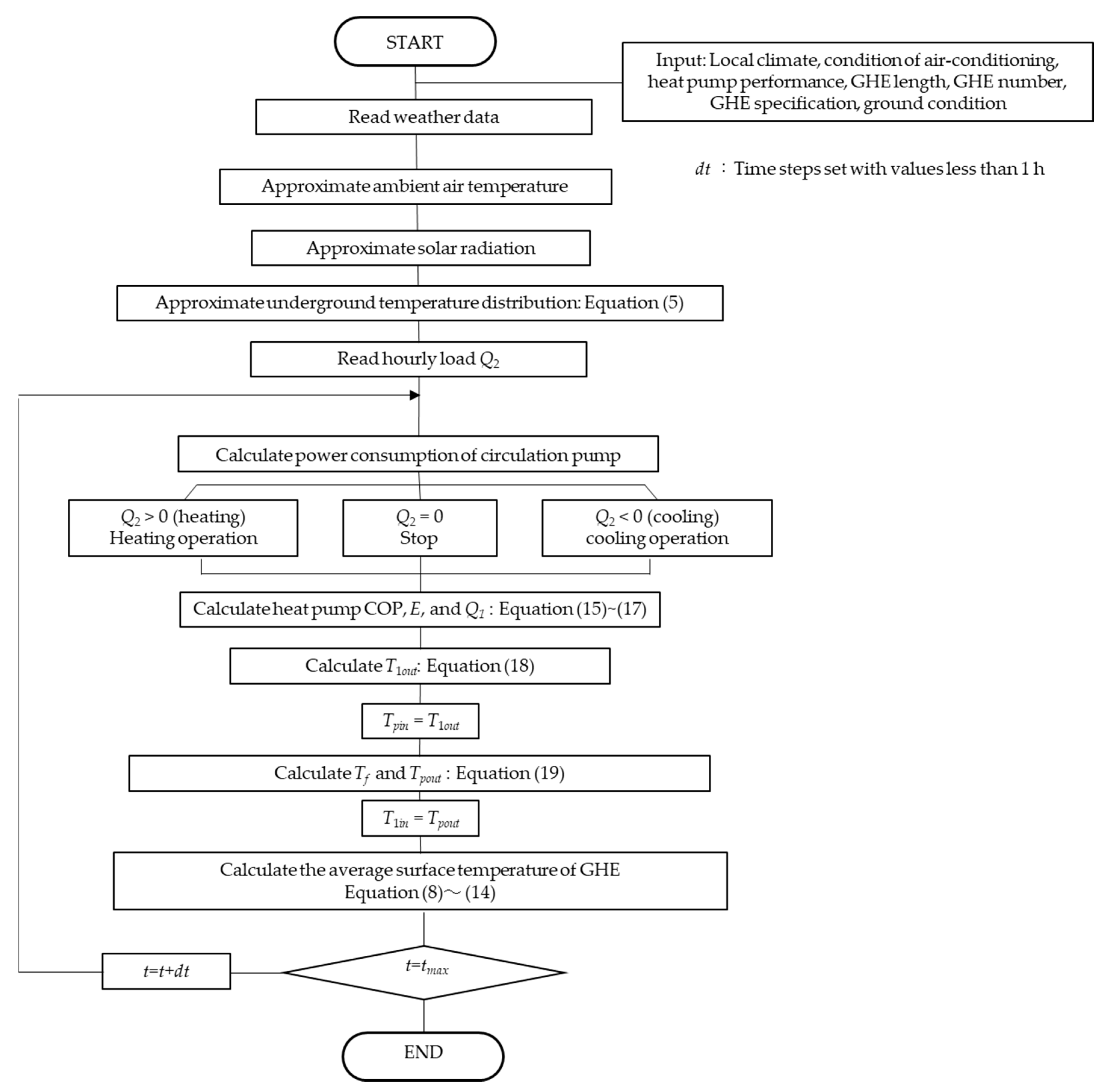
If these calculations are carried out repeatedly, the hourly temperature variation can be obtained. Figure 2 shows a calculation flow of the simulation tool. This tool calculates the approximate expression of the ground temperature distribution from the weather data before simulating the performance of the GSHP system and calculates the average temperature variation caused by the underground temperature distribution from the approximate expression. Consequently, this simulation tool can consider the influence of ground surface.
3. Thermal Response Test to Validate Calculation Result
3.1. Thermal Response Test
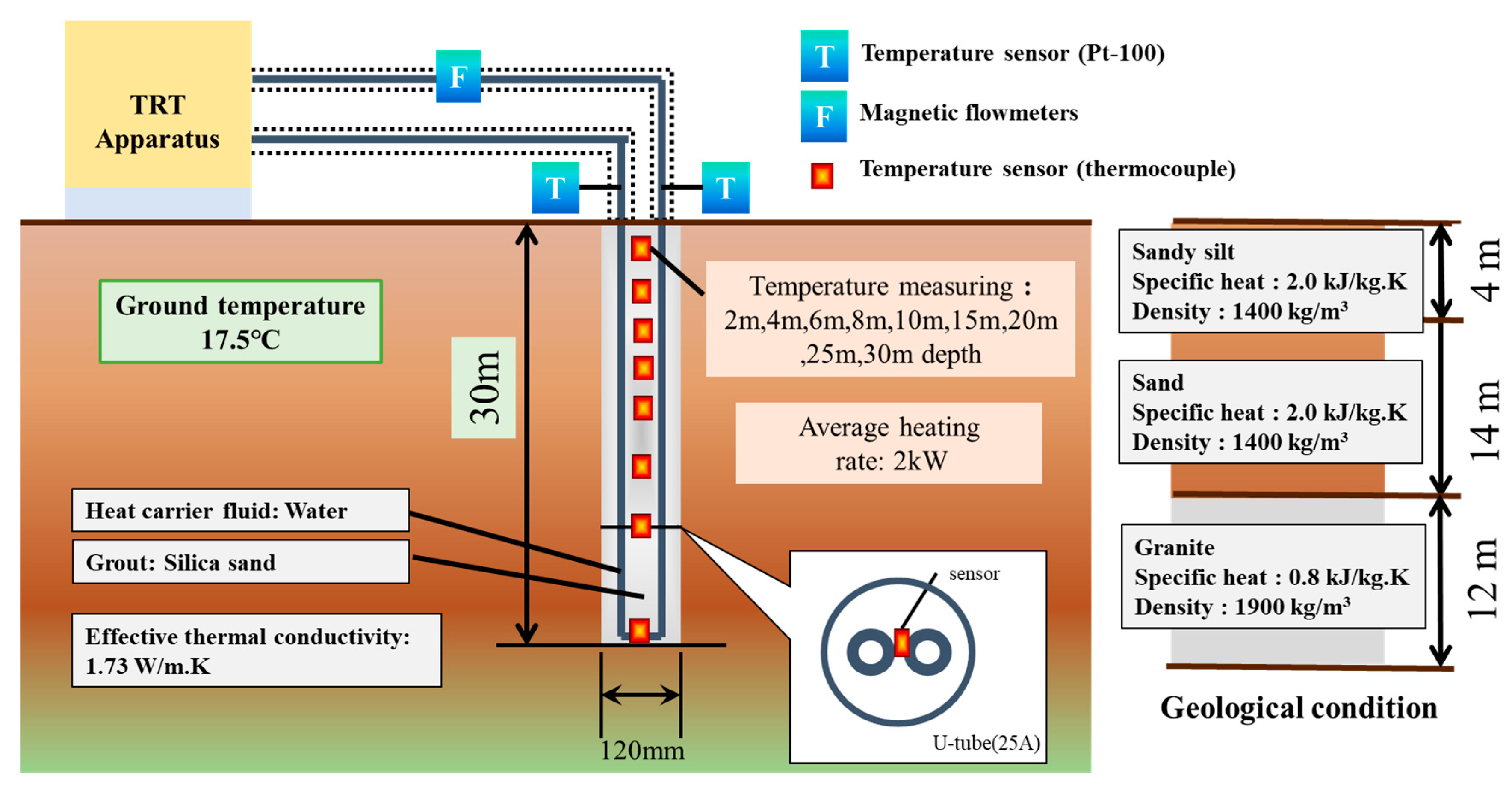
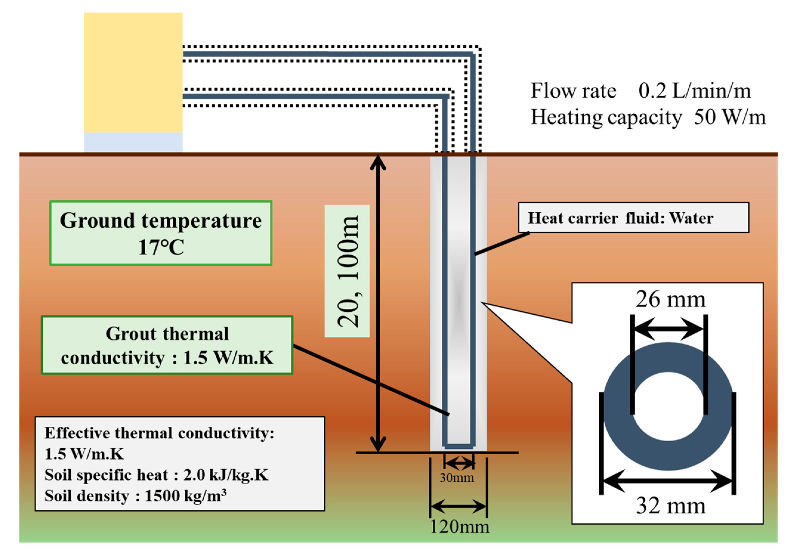
To validate the accuracy of the simulation tool, a thermal response test (TRT) was performed as shown in Figure 3. The test was conducted at a private company’s field in Karatsu City, Saga Prefecture, for two days from March 11 to 13, 2013. Using an electric boiler and a circulating pump, water was circulated at a constant flow rate and heating rate (average 2 kW) to inject heat into the ground. The temperatures of the U-tube surface inside the borehole GHE were measured using thermocouples at 9 depths: 2 m, 4 m, 6 m, 8 m, 10 m, 15 m, 20 m, 25 m and 30 m. In addition, the inlet and outlet temperature of the GHE were measured using Pt-100 temperature sensors and the flow rate was measured using an electromagnetic flowmeter.
3.2. Calculation Conditions
Table 1 shows the calculation conditions. The conditions of the GHE and soil were set so as to be the same as the measurement. The underground geology is sandy silt up to a depth of 4 m, sand from 4 m to 18 m and weathered granite from 18 m to 30 m. The values of soil density and specific heat were estimated for these geological conditions as shown in Figure 4, and the weighted average was calculated based on the thickness. The value of effective thermal conductivity from a previously performed TRT was given. Silica sand was used as grouting material. As a condition for the simulation, the grout (silica sand) thermal conductivity is considered to be about 1.8 W/m.K. However, there is a possibility that convection may occur, thus in consideration of the effect, the value was doubled to 3.6 W/m.K. In the simulation, the measured values of the heating rate and the flow rate were given hourly, and the temperature of the heat carrier fluid in the GHE and the temperature of the GHE at a depth of 2 m, 6 m and 10 m were calculated.
In addition, the weather data at Esashiki (Saga Prefecture), which is the closest to the test site, was used to calculate the underground temperature distribution. When comparing the borehole inside temperatures, the borehole surface temperature was calculated in the simulation, while the U-tube surface temperature were measured by placing the temperature sensor in the middle of the inlet and the outlet pipe in the TRT, as shown in Figure 4. Therefore, the surface temperature was calculated using Equation (20) to compare and validate.
Here, is the heat injection rate (negative value of the heat extraction rate), is the overall heat transfer coefficient from the borehole surface to the U-tube surface, and is the surface area of the borehole. was obtained using the boundary element method shown in the previous research [16].
3.3. Result and Discussion
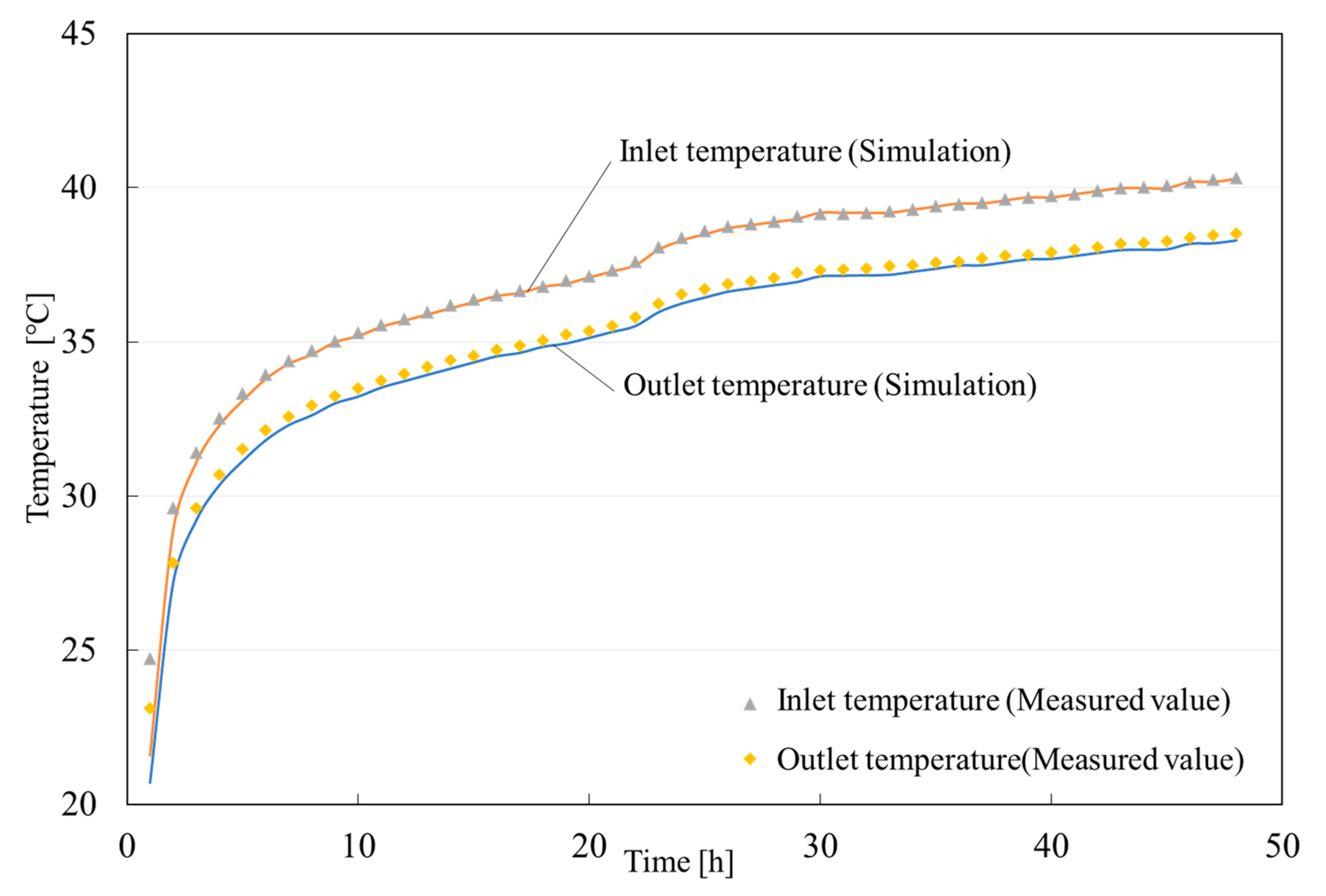
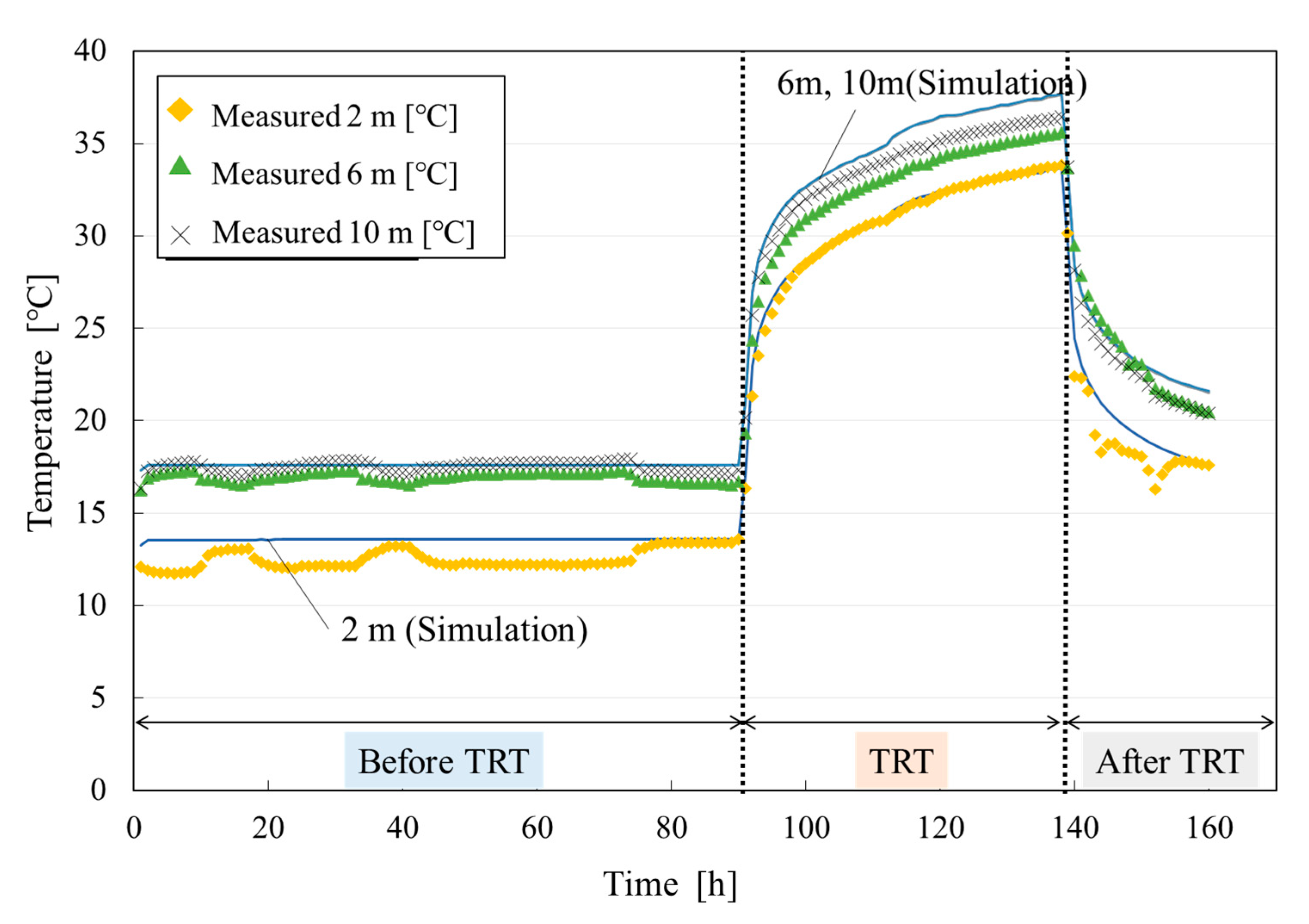
The temperatures of heat carrier fluid at inlet and outlet of the GHE in the TRT were measured and calculated, and they were compared as shown in Figure 4. In addition, the variations of U-tube surface temperature at different depths obtained using the measurement and calculation are shown in Figure 5.
According to the results, the average relative error of the temperatures of the heat carrier fluid between the measurement and calculation is 3.3%. This value shows acceptable precision. When comparing the U-tube surface temperature during the TRT, the difference between the temperatures was hardly observed at a depth of 2 m. The differences between the temperatures at the depth of 6 m and 10 m are approximately 1~2 °C. Therefore, this simulation tool can reproduce the measurement within an allowable range.
In addition, it is considered that the calculated value of the temperature variation after the TRT well reproduces the practically measured value.
4. Evaluation on Influence of Surface Temperature during Thermal Response Test
4.1. Calculation Conditions
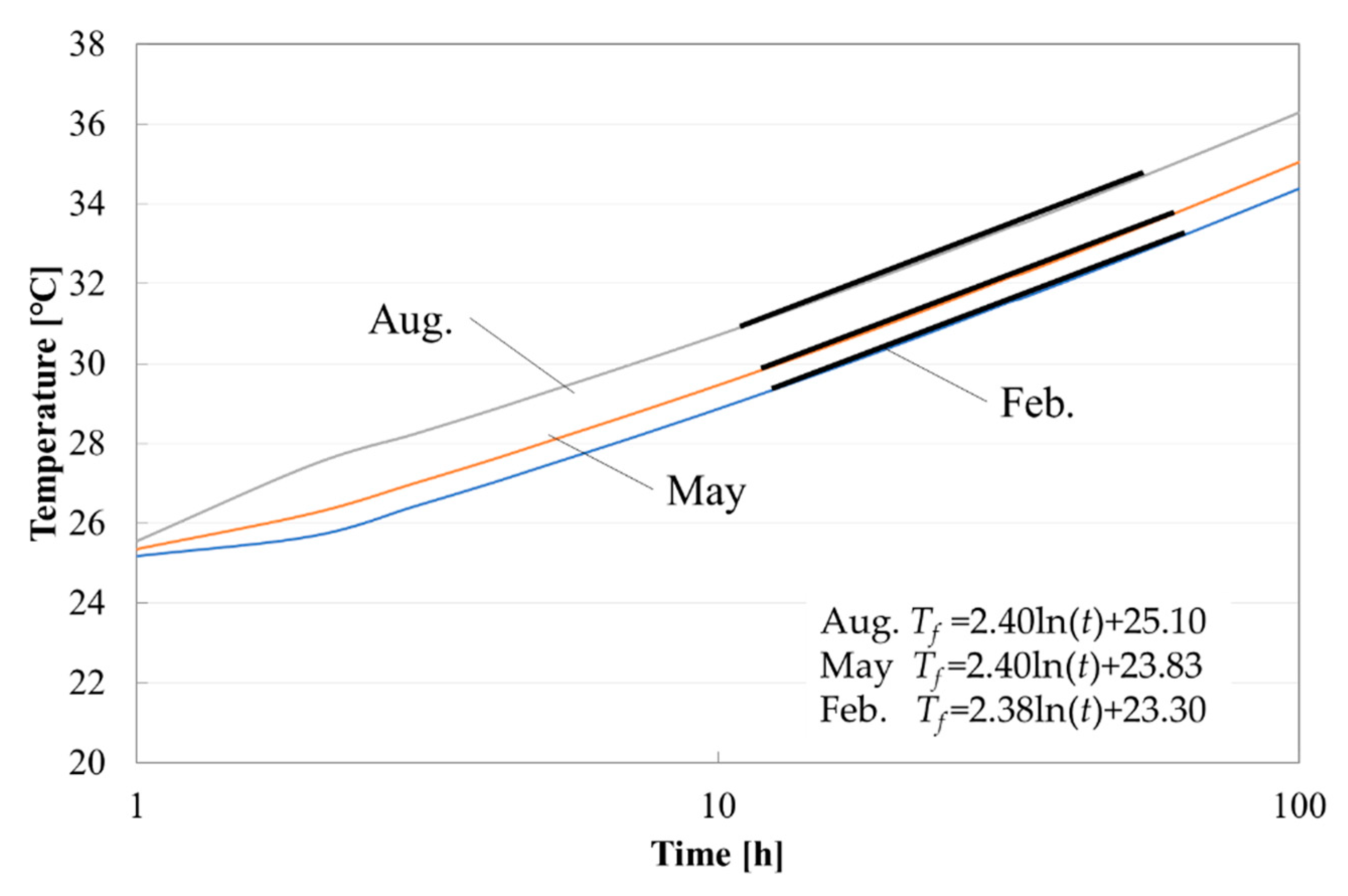
The influence of the ground surface on the temperature variation during the TRT, as shown in Figure 6, was evaluated using the developed tool. GHEs with borehole lengths of 20 m and 100 m were used and three meteorological conditions for February, May, and August were set. The temperature variations of the heat carrier fluid in the GHE were calculated and the results were compared. Table 2 shows the calculation conditions. As other calculation conditions, a constant flow rate of 0.2 L/min/m (4 L/min for GHE with 20 m long and 20 L/min for GHE with 100 m long) and a heating rate of 50 W/m (1 kW for GHE with 20 m long and 5 kW for GHE with 100 m long) were given. The values of the GHE and soil were assumed to be general values in Japan. The calculation period was 100 h. Yahata (Kitakyushu) was selected as the area to give the weather data.
4.2. Result and Discussion
Figure 7 and Figure 8 show the variations of the heat carrier fluid in the GHE with the different borehole lengths. When the borehole length of the GHE was set to 20 m, there was a temperature difference of approximately 2 °C between winter and summer, and a difference in the temperature gradient for the first several hours was observed due to the influence of the ground surface. However, when the gradients of logarithmic approximation obtained from the temperature variations were compared, it was found that there was no significant difference. In addition, when the borehole length of the GHE was set to 100 m, a difference in the temperature variation was hardly observed. As a result, it is confirmed that the influence of the ground surface on the TRT results such as the effective thermal conductivity is small even when a GHE with a borehole length of 20 m is used.
5. Evaluation on Influence of Ground Surface on GSHP System Performance
5.1. Calculation Conditions
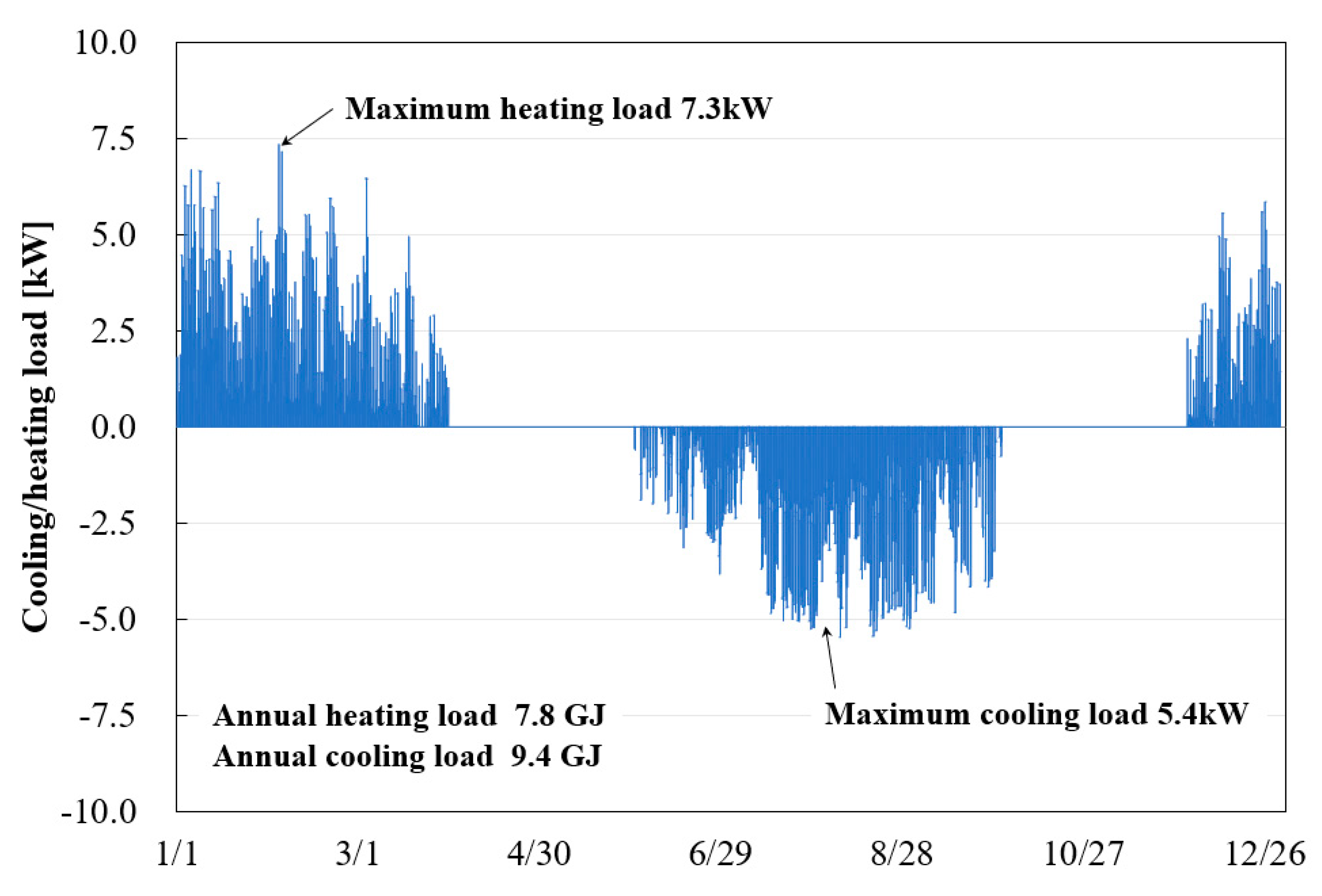
Assuming that the GSHP system is installed in a residential house in a moderate climate area, the effect of the short GHE on the system performance is investigated. Table 3 shows the calculation conditions. The building is a standard house set by the Japan Architectural Association. The air-conditioning section is set to the temperature and humidity shown in Table 3. The heating and cooling load under this condition is calculated using the building energy simulation tool BEST [25].
Figure 9 shows the time-dependent fluctuation of the heating and cooling load of the building. The heat source equipment used in this house is assumed to be a small-capacity water-cooled package air-conditioning heat pump. The total borehole length of the GHE was set to be 100 m, and the calculation was performed under four conditions of 100 m × 1 borehole, 50 m × 2 boreholes, 20 m × 5 boreholes and 10 m × 10 boreholes. In the case of multiple GHEs, the GHEs are arranged in a horizontal row at intervals of 5 m and connected in series to each other. Single U-tube was used, and general values were given for soil conditions. Two types of soil effective thermal conductivity, 1.0 W/m.K for considering unsaturated soil and 1.5 W/m.K for considering saturated soil, are given. Yahata (Kitakyushu) was selected as the area to give the weather data. The calculation period is two years. After changing the length condition as described above, the monthly ground temperature variation, power consumption, etc. in the second year were calculated and compared.
5.2. Result and Discussion
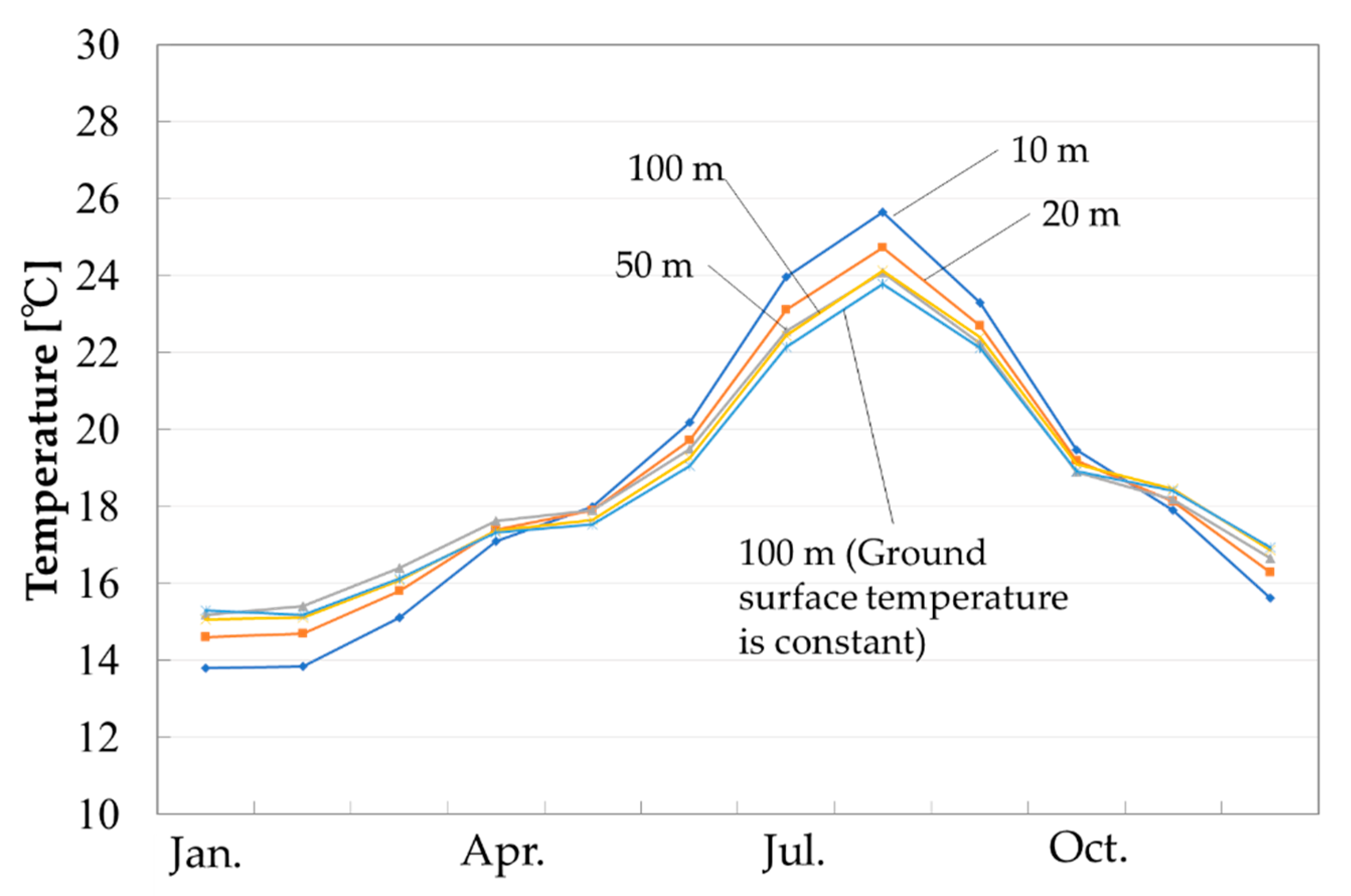
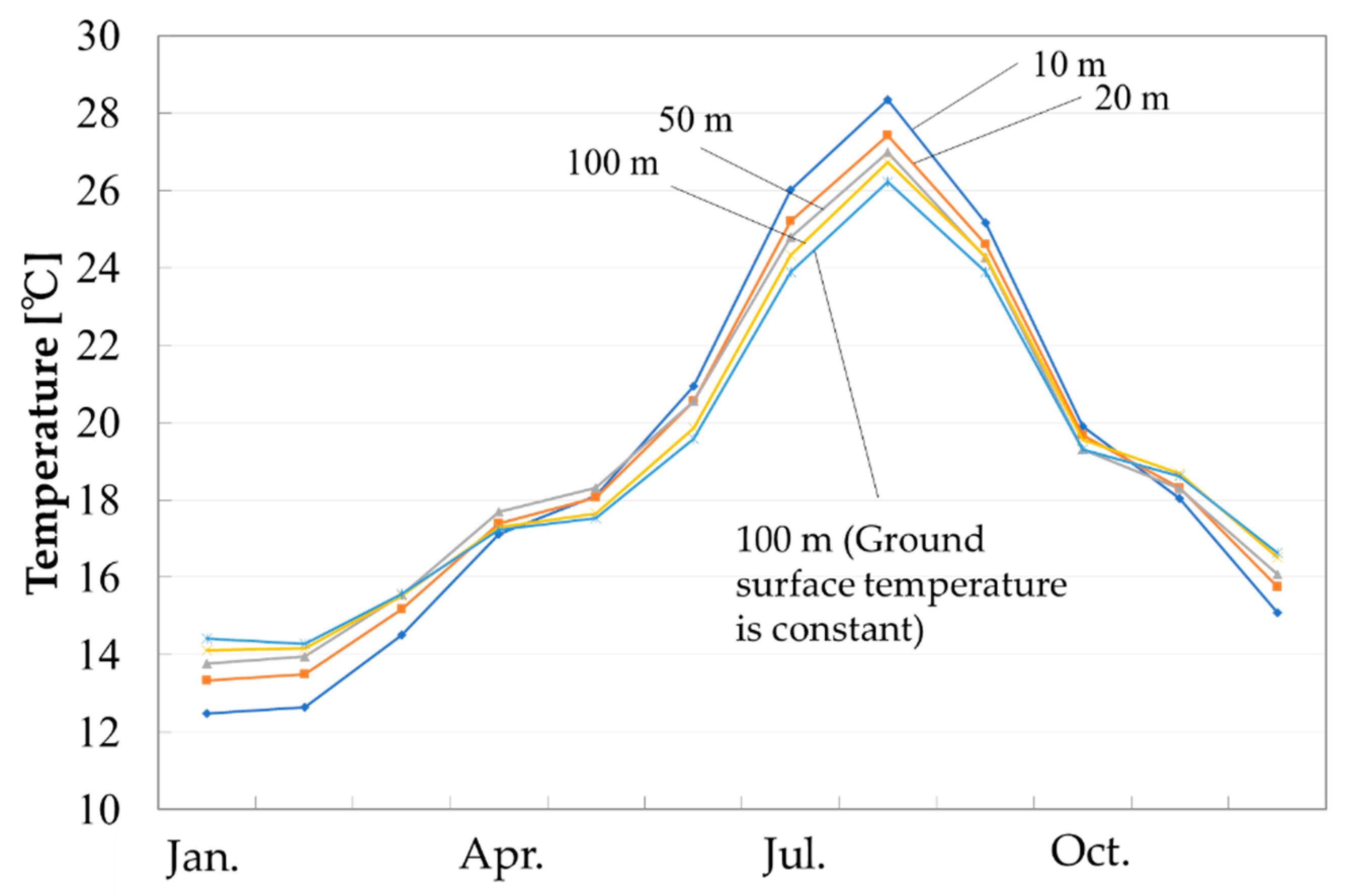
Figure 10 and Figure 11 show the monthly variations of the average surface temperature of the GHE with different borehole lengths. The effective thermal conductivity of soil is set to 1.5 W/m.K in Figure 10 and 1.0 W/m.K in Figure 11. Figure 10 and Figure 11 also show the monthly variation of the average surface temperature of the GHE when the boundary condition of the ground surface is set as the constant temperature condition (17.8 °C). When the soil effective thermal conductivity is lower (1.0 W/m.K), the average surface temperature of the GHE during the cooling season is approximately from 2 to 4 °C higher compared to a temperature for the condition of soil effective thermal conductivity of 1.5 W/m.K. In addition, the average surface temperature of the GHE during the heating season is approximately 1 °C lower.
Under the condition that the borehole length and number of the GHE are 100 m and 1 borehole (with or without considering the temperature variation of the ground surface), the results show that the temperatures in the two cases have a difference of from 0.3 to 0.5 °C during cooling and from 0.2 to 0.3 °C during heating, respectively.
The comparison of temperature variations with the different borehole length conditions shows that the GHE with the shorter borehole length and the larger number yields larger temperature variation. If the influence of ground surface (temperature variation on the ground surface) is considered, the average surface temperature of the GHE with the borehole length of 10 m becomes approximately 2 °C higher than the average surface temperature of the GHE with the borehole length of 100 m in August, regardless of the effective thermal conductivity. In January, the average surface temperature of the GHE with the borehole length of 10 m decreases 2 °C more, while the influence of ground surface on the condition of borehole length of 20 m is less than the case of 10 m.
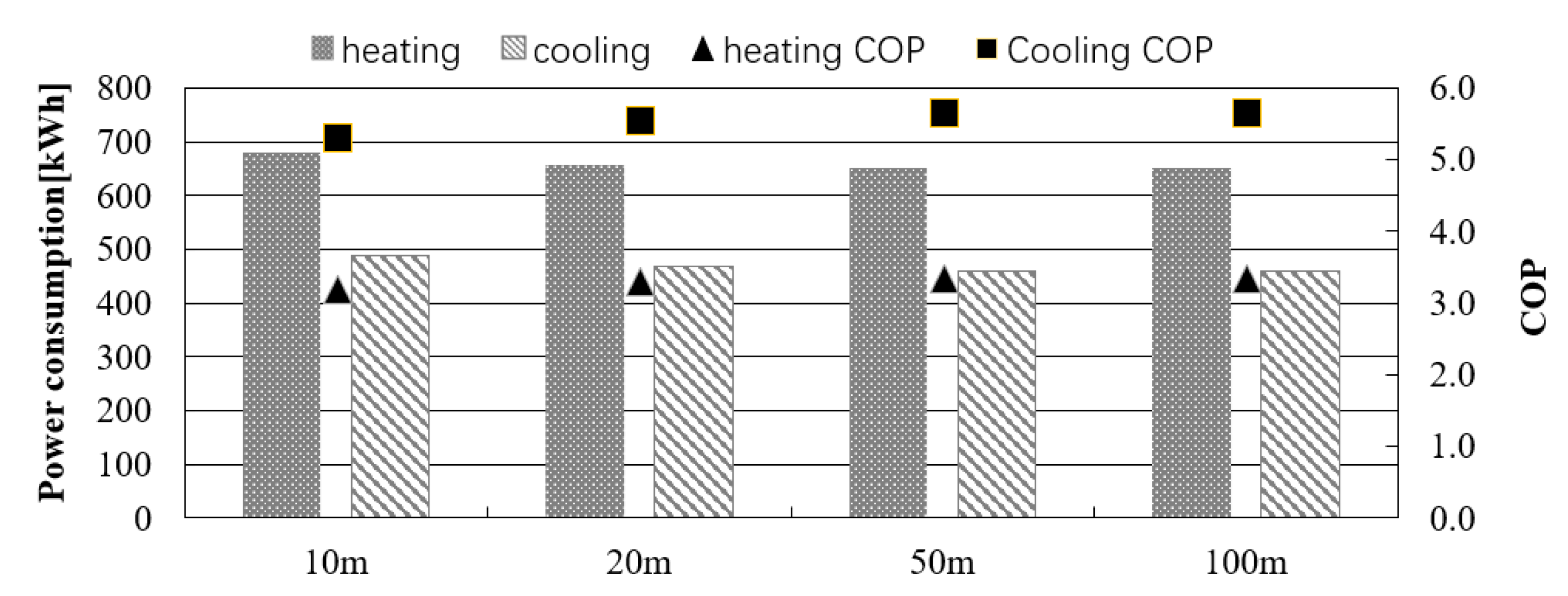
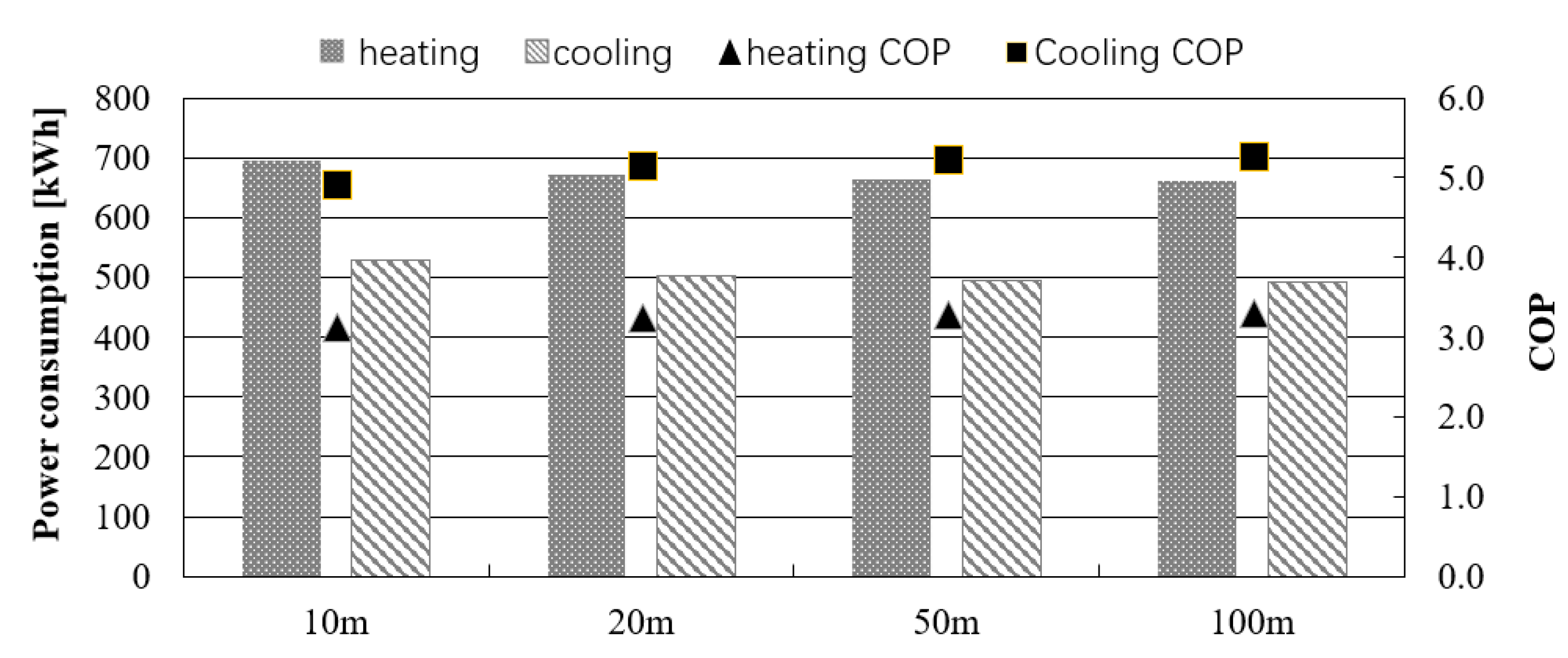
Figure 12 and Figure 13 show the electric power consumption of the heat pump unit and the average COPs in season for the conditions of different borehole length. Figure 13 shows the results for a soil thermal conductivity of 1.5 W/m.K, and Figure 14 shows the results for 1.0 W/m.K. When the electric power consumption for the conditions of borehole length of 10 m (×10 boreholes) and 100 m (×1 borehole) are compared, the electric power consumption for the condition of borehole length of 10 m increases 8.1% in the cooling season. Similarly, the electric power consumption for the condition of borehole length of 10 m increases 2.4% in the heating season. When the COPs are compared, it was found that the COP in the case of a 10 m borehole length decreases by 0.5 during the cooling season compared to the COP in the case of a 100 m borehole length.
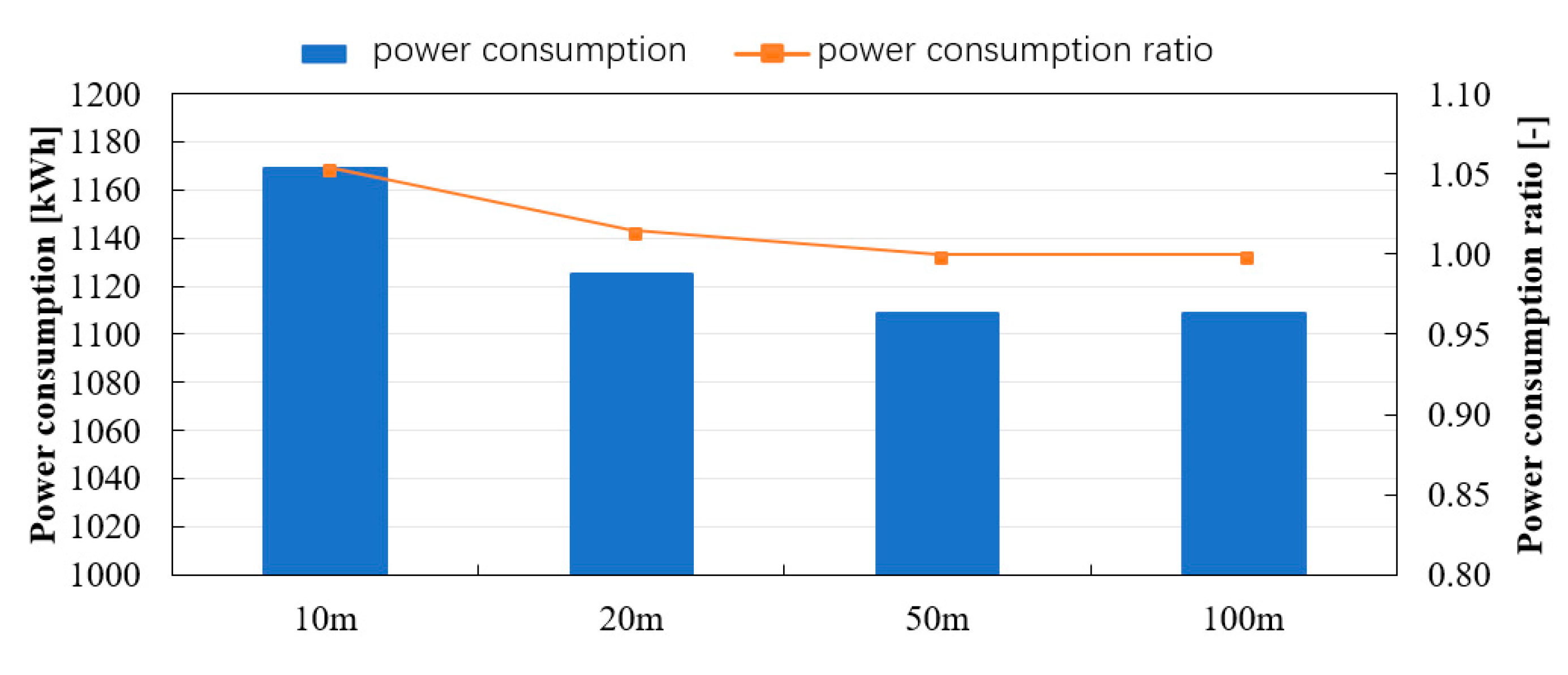
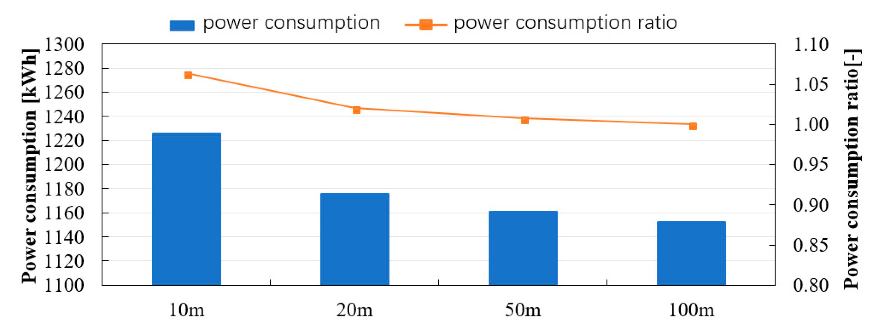
Finally, Figure 14 and Figure 15 show the annual energy consumption for the different borehole lengths and the ratios when 100 m × 1 borehole is set to 1. Annual energy consumption increased by 5 to 6% for 10 m GHEs compared to a 100 m GHE, however, it increased only approximately 2% for 20 m GHEs. From this, it was confirmed that the performance of the GSHP system using GHEs with the borehole length of 20 m was not significantly decreased compared with the GSHP system using a GHE with a borehole length of 100 m.
6. Conclusions
- (1)
- By applying the superposition theorem, the authors developed a GHE calculation model considering the influence of the ground surface. In addition, the GHE calculation model was combined with a simulation tool for a GSHP system. The outlines of the calculation model for a short GHE were explained.
- (2)
- A TRT was carried out using a GHE with a borehole length of 30 m, and the heat carrier fluid temperature in the GHE and the underground temperature were obtained using measurements. The results were then compared with the results from the simulation. The relative error of the temperature of the heat carrier fluid was 3.3%. This result indicated that the tool can reproduce the measurements with acceptable precision.
- (3)
- The influence of the ground surface on the TRT result was investigated using the developed tool. The result showed that the difference of the effective thermal conductivities obtained from TRTs for different seasons is small even when a GHE with a borehole length of 20 m is used.
- (4)
- It was assumed that the GSHP system is installed in a residential house to discuss the influence of the ground surface temperature on the temperature variation of heat carrier fluid in GHEs and the performance of the GSHP system. Comparing the calculation results of GHEs with borehole lengths of 10 m and 100 m under the same total length of GHEs and the same effective thermal conductivity, it was found that the average surface temperature of a GHE with a borehole length of 10 m becomes approximately 2 °C higher than the average surface temperature of a GHE with a borehole length of 100 m in August. Comparing the annual power consumption, a GSHP system using 10 GHEs with the borehole length of 10 m increases the consumption by 5 to 6% compared to a GSHP system using one GHE with the borehole length of 100 m. In the case of the GHE with a borehole length of 20 m, it was found that the increase of annual power consumption was only about 2%.
Author Contributions
Conceptualization, T.K.; data curation, T.K. and L.D.; investigation, T.K.; project administration, T.K.; supervision, Y.S. and K.N.; validation, T.K.; writing—original draft, T.K. and L.D. All authors have read and agreed to the published version of the manuscript.
Funding
This research was funded by NEDO grant number P14017.
Acknowledgments
This study is based on results obtained from the project “Renewable energy heat utilization technology development,” commissioned by the Japan national agency New Energy and Industrial Technology Development Organization (NEDO). In addition, the authors would like to express appreciation to Motohiro Hirata for supporting this research.
Conflicts of Interest
The authors declare no conflict of interest.
Nomenclature
| A | Area [m2] |
| a | Solar radiation absorption rate [-] |
| C | Correction coefficient [-] |
| c | Specific heat [kJ/kg.K] |
| cp | Specific heat at constant pressure [kJ/kg.K] |
| E | Electric power consumption of heat pump unit [W] |
| G | Flow rate [m3/s] |
| I | Total solar radiation [W/m2] |
| J | Effective radiation [W/m2] |
| K | Overall heat transfer coefficient [W/m2.K] |
| L | Length [m] |
| l | Parameter relating to length [m] |
| N | Number of time step [-] |
| Q | Heating load [W] |
| q | Heat extraction rate [W/m] |
| r | Radius [m] |
| r* | Non-dimensional distance (=r/rp) [-] |
| T | Temperature [°C] |
| T* | Non-dimensional temperature (=λΔT/r/q) [-] |
| t | Time [s] |
| tc | Time starting from July 1 [h] |
| t* | Fourier number (=at/r2) [-] |
| V | Volume [m3] |
| Z | Depth [m] |
| α | Total heat transfer coefficient [W/m2.K] |
| β | Characteristic value [-] |
| ε | Emissivity [-] |
| 𝜆 | Thermal conductivity [W/m.K] |
| 𝜌 | Density [kg/m3] |
| 𝜓 | Equivalent outside air temperature on the ground surface [°C] |
| 𝜔 | Angular velocity (=2π/8760) [-] |
| Subscripts | |
| 1 | Heat pump primary side |
| 1f | Heat carrier fluid in the primary side |
| 1in | Inlet in the primary side |
| 1out | Outlet in the primary side |
| 2 | Heat pump secondary side |
| a | Ambient air |
| C | Temperature response of cylindrical heat sources |
| d | Distance |
| f | Heat carrier fluid (water or antifreeze liquid) |
| I | Solar radiation |
| J | Effective radiation |
| L | Temperature response of line heat source |
| p | Ground heat exchanger |
| pin | Inlet of ground heat exchanger |
| pout | Outlet of ground heat exchanger |
| p-in | Inside of ground heat exchanger |
| p-out | Outside of ground heat exchanger |
| s | Soil |
| s0 | Soil initial |
| s1 | Soil affected by the heat injection/extraction via GHEs |
| s2 | Soil affected by the underground temperature distribution |
| t | Affected by ambient air temperature |
| U-out | U-tube outside |
| -ave | Average |
References
- John, W.L.; Derek, H.F.; Tonya, L.B. Direct Utilization of Geothermal Energy 2010 Worldwide Review. Geothermics 2010, 40, 159–180. [Google Scholar]
- Zarrella, A.; De Carli, M. Heat transfer analysis of short helical borehole heat exchangers. Appl. Energy 2013, 102, 1477–1491. [Google Scholar] [CrossRef]
- Zarrella, A.; Capozza, A.; De Carli, M. Analysis of short helical and double U-tube borehole heat exchangers: A simulation-based comparison. Appl. Energy 2013, 112, 358–370. [Google Scholar] [CrossRef]
- Zarrella, A.; Emmi, G.; De Carli, M. Analysis of operating modes of a ground source heat pump with short helical heat exchangers. Energy Convers. Manag. 2015, 97, 351–361. [Google Scholar] [CrossRef]
- Hamada, Y.; Saitoh, H.; Nakamura, M.; Kubota, H.; Ochifuji, K. Field performance of an energy pile system for space heating. Energy Build. 2007, 39, 517–524. [Google Scholar] [CrossRef]
- Katsura, T.; Nagano, K.; Narita, S.; Takeda, S.; Nakamura, Y.; Okamoto, A. Calculation Algorithm of the Temperatures for Pipe Arrangement of Multiple Ground Heat Exchangers. Appl. Therm. Eng. 2009, 29, 906–919. [Google Scholar] [CrossRef]
- Katsura, T.; Nagano, K.; Sakata, Y.; Wakayama, H. A design and simulation tool for ground source heat pump system using energy piles with large diameter. Int. J. Energy Res. 2019, 43, 1505–1520. [Google Scholar] [CrossRef]
- Fujii, H.; Nishi, K.; Komaniwa, Y.; Chou, N. Numerical modeling of slinky-coil horizontal ground heat exchangers. Geothermics 2012, 41, 55–62. [Google Scholar] [CrossRef]
- Fujii, H.; Yamasaki, S.; Maehara, T.; Ishikami, T.; Chou, N. Numerical simulation and sensitivity study of double-layer Slinky-coil horizontal ground heat exchangers. Geothermics 2013, 47, 61–68. [Google Scholar] [CrossRef]
- Li, H.; Nagano, K.; Lai, Y. A New Model and Solutions for a Spiral Heat Exchanger and Its Experimental Validation. Int. J. Heat Mass Transf. 2012, 55, 4404–4414. [Google Scholar] [CrossRef]
- Li, H.; Nagano, K.; Lai, Y. Heat transfer of a horizontal spiral heat exchanger under groundwater advection. Int. J. Heat Mass Transf. 2012, 55, 6819–6831. [Google Scholar] [CrossRef]
- Xiong, Z.; Fisher, D.E.; Spitler, J.D. Development and validation of a Slinky ground heat exchanger model. Appl. Energy 2015, 141, 57–69. [Google Scholar] [CrossRef]
- Hamada, Y.; Nakamura, M.; Yokoyama, S.; Nagano, K.; Nagasaka, S.; Ochifuji, K. Study on Prediction of Underground Temperature for Utilizing Underground Heat in Snowy Area. Trans. Soc. Heat. Air Condit. Sanit. Eng. Jpn. 1998, 23, 91–100. [Google Scholar]
- Eckert, E.R.G.; Drake, R.M. Analysis of Heat and Mass Transfer; McGraw-Hill Kogakusha. Ltd.: Tokyo, Japan, 1972; pp. 208–214. [Google Scholar]
- Bandos, T.V.; Montero, A.; Fernandez, E.; Santander, J.L.G.; Isidro, J.M.; Pérez, J.; De Córdoba, P.J.F.; Urchueguía, J.F. Finite Line-source Model for Borehole Heat Exchangers Effect of Vertical Temperature Variations. Geothermics 2009, 38, 263–270. [Google Scholar] [CrossRef]
- Nagano, K.; Katsura, T.; Takeda, S. Development of a Design and Performance Prediction Tool for the Ground Source Heat Pump System. Appl. Therm. Eng. 2006, 26, 1578–1592. [Google Scholar] [CrossRef]
- Katsura, T.; Nagano, K.; Takeda, S. Method of Calculation of the Ground Temperature for Multiple Ground Heat Exchangers. Appl. Therm. Eng. 2008, 28, 1995–2004. [Google Scholar] [CrossRef]
- Morchio, S.; Fossa, M. On the ground thermal conductivity estimation with coaxial borehole heat exchangers according to different undisturbed ground temperature profiles. Appl. Therm. Eng. 2020, 173, 115198. [Google Scholar] [CrossRef]
- Nagasaka, S.; Ochifuji, K.; Nagano, K.; Yokoyama, S.; Nakamura, M.; Hamada, Y. An Estimate of the Surface Temperature at a Vertical Ground Pipe by Line Source Theory. Trans. Soc. Heat. Air Condit. Sanit. Eng. Jpn. 1995, 20, 143–152. [Google Scholar]
- Ochifuji, K.; Suzuki, M.; Nakamura, M. Study on Characteristics of Long-Term Underground Heat Storage of Solar Vertical Tube System and Its Application to Heating (1st Report). Trans. Soc. Heat. Air Condit. Sanit. Eng. Jpn. 1985, 10, 95–106. [Google Scholar]
- Architectural Institute of Japan. Extended AMeDAS Meteorological Data 1981–2000; Architectural Institute of Japan: Tokyo, Japan, 2005. [Google Scholar]
- ASHRAE. Ground Source Heat Pumps Design of Geothermal System for Commercial and Institutional Buildings; American Society of Heating, Refrigerating and Air-Conditioning Engineers: Atlanta, GA, USA, 1997. [Google Scholar]
- Fossa, M. Correct design of vertical borehole heat exchanger systems through the improvement of the ASHRAE method. Sci. Technol. Built. Eng. 2017, 23, 1080–1089. [Google Scholar] [CrossRef]
- Katsura, T.; Higashitani, T.; Fang, Y.; Sakata, Y.; Nagano, K.; Akai, H.; Oe, M. A New Simulation Model for Vertical Spiral Ground Heat Exchangers Combining Cylindrical Source Model and Capacity Resistance Model. Energies 2020, 13, 1339. [Google Scholar] [CrossRef] [Green Version]
- BEST-P Building Operation Manual. Available online: http://www.ibec.or.jp/best/program/manual/ (accessed on 20 May 2020).
Figure 1.
Schematic diagram of measuring underground temperature (left) and comparison between calculated and measured temperature (right).
Figure 1.
Schematic diagram of measuring underground temperature (left) and comparison between calculated and measured temperature (right).

Figure 2.
Performance prediction tool calculation flow considering influence of ground surface.

Figure 3.
Diagram of thermal response test.

Figure 4.
Comparison of temperature variations of GHE inlet/outlet.

Figure 5.
Comparison of U-tube surface temperatures at each depth.

Figure 6.
Schematic diagram of the TRT.

Figure 7.
Comparison of temperature variations of heat carrier fluid for each season (20 m).

Figure 8.
Comparison of temperature variations of heat carrier fluid for each season (100 m).

Figure 9.
Total heating and cooling load of a residential house.

Figure 10.
Monthly variations of the average surface temperature of GHE. (Effective thermal conductivity 1.5 W/m.K).
Figure 10.
Monthly variations of the average surface temperature of GHE. (Effective thermal conductivity 1.5 W/m.K).

Figure 11.
Monthly variations of the average surface temperature of GHE. (Effective thermal conductivity 1.0 W/m.K).
Figure 11.
Monthly variations of the average surface temperature of GHE. (Effective thermal conductivity 1.0 W/m.K).

Figure 12.
Electric power consumption and average COPs for different length of GHE. (Effective thermal conductivity 1.5 W/m.K).
Figure 12.
Electric power consumption and average COPs for different length of GHE. (Effective thermal conductivity 1.5 W/m.K).

Figure 13.
P Electric power consumption and average COPs for different length of GHE. (Effective thermal conductivity 1.0 W/m.K).
Figure 13.
P Electric power consumption and average COPs for different length of GHE. (Effective thermal conductivity 1.0 W/m.K).

Figure 14.
Total energy consumption for different length of GHE. (Effective thermal conductivity 1.5 W/m.K).
Figure 14.
Total energy consumption for different length of GHE. (Effective thermal conductivity 1.5 W/m.K).

Figure 15.
Total energy consumption for different length of GHE. (Effective thermal conductivity 1.0 W/m.K).
Figure 15.
Total energy consumption for different length of GHE. (Effective thermal conductivity 1.0 W/m.K).


Table 1.
Calculation conditions.
| GHEX | specification | Borehole U-tube |
| Boundary condition of ground surface | Temperature boundary condition | |
| Number of U-tube | 1 | |
| U-tube interval | 0.03 m | |
| Borehole length and number | 1 × 30 m | |
| Borehole diameter | 0.12 m | |
| U-tube outside diameter | 0.032 m | |
| U-tube inside diameter | 0.026 m | |
| Grout thermal conductivity | 3.6 W/m.K | |
| Soil | Density of soil | 1600 kg/m3 |
| Undisturbed temperature | 17.5 °C | |
| Specific heat capacity | 1.5 kJ/kg.K | |
| Effective thermal conductivity | 1.73 W/m.K | |
| Heat carrier fluid | Type | Water |
| Density | 1000 kg/m3 | |
| Specific heat at constant pressure | 4.187 kJ/kg.K |
Table 2.
Calculation condition.
| GHE | Specification | Borehole U-tube |
| Boundary condition of ground surface | Temperature boundary condition | |
| Number of U-tube | 1 | |
| U-tube interval | 0.03 m | |
| Borehole length and number | 20 m or 100 m × 1 | |
| Borehole diameter | 0.12 m | |
| U-tube outside diameter | 0.032 m | |
| U-tube inside diameter | 0.026 m | |
| Grout thermal conductivity | 1.5 W/m.K | |
| Density of soil | 1500 kg/m3 | |
| Soil | Undisturbed temperature | 17.0 °C |
| Specific heat capacity | 2.0 kJ/kg.K | |
| Effective thermal conductivity | 1.5 W/m.K | |
| Heat carrier fluid | Type | Water |
| Density | 1000 kg/m3 | |
| Specific heat at constant pressure | 4.187 kJ/kg.K |
Table 3.
Calculation condition.
| Building | Wooden house | |
| Area | 120 m2 | |
| City | Yahata (Kitakyushu) | |
| Heat loss coefficient (Q-value) | 2.7 W/m2.K | |
| Ventilation | 0.5 times/h | |
| Air conditioning area | 55% | |
| Preset temperature and humidity | Cooling 27 °C, 60% Heating 20 °C, 50% | |
| Heat pump | Water-cooled package air-conditioning heat pump | |
| Rated heating output | 12.5 kW | |
| Rated power consumption for heating | 3.2 kW | |
| Rated cooling output | 11.2 kW | |
| Rated power consumption for cooling | 3.1 kW | |
| Flow rate of circulation pump | 25 L/min | |
| Power consumption of circulation pump | 0.1 kW | |
| GHE | Specification | Borehole U-tube |
| Boundary condition of ground surface | Temperature boundary condition | |
| Number of U-tube | 1 | |
| U-tube interval | 0.03 m | |
| Borehole length | 10 m, 20 m, 50 m, 100 m | |
| Diameter of borehole | 0.12 m | |
| U-tube outside diameter | 0.032 m | |
| U-tube inside diameter | 0.026 m | |
| Grout thermal conductivity | 1.8 W/m.K | |
| Soil | Density of soil | 1600 kg/m3 |
| Undisturbed temperature | 17.8 °C | |
| Specific heat capacity | 1.5 kJ/kg.K | |
| Effective thermal conductivity | 1.5 W/m.K 1.0 W/m.K | |
| Heat carrier fluid | Type | Water |
| Density | 1000 kg/m3 | |
| Specific heat at constant pressure | 4.187 kJ/kg.K | |
© 2020 by the authors. Licensee MDPI, Basel, Switzerland. This article is an open access article distributed under the terms and conditions of the Creative Commons Attribution (CC BY) license (http://creativecommons.org/licenses/by/4.0/).
Share and Cite
MDPI and ACS Style
Katsura, T.; Sakata, Y.; Ding, L.; Nagano, K. Development of Simulation Tool for Ground Source Heat Pump Systems Influenced by Ground Surface. Energies 2020, 13, 4491. https://doi.org/10.3390/en13174491
AMA Style
Katsura T, Sakata Y, Ding L, Nagano K. Development of Simulation Tool for Ground Source Heat Pump Systems Influenced by Ground Surface. Energies. 2020; 13(17):4491. https://doi.org/10.3390/en13174491
Chicago/Turabian StyleKatsura, Takao, Yoshitaka Sakata, Lan Ding, and Katsunori Nagano. 2020. "Development of Simulation Tool for Ground Source Heat Pump Systems Influenced by Ground Surface" Energies 13, no. 17: 4491. https://doi.org/10.3390/en13174491
Note that from the first issue of 2016, this journal uses article numbers instead of page numbers. See further details here.