Multiphysics CFD Simulation for Design and Analysis of Thermoelectric Power Generation


Department of Chemistry and Chemical Engineering, Chalmers University of Technology, SE-41296 Gothenburg, Sweden
*
Author to whom correspondence should be addressed.
Energies 2020, 13(17), 4344; https://doi.org/10.3390/en13174344
Submission received: 30 July 2020
/
Revised: 18 August 2020
/
Accepted: 20 August 2020
/
Published: 22 August 2020
(This article belongs to the Special Issue Engineering Fluid Dynamics 2019-2020)
Abstract
:The multiphysics simulation methodology presented in this paper permits extension of computational fluid dynamics (CFD) simulations to account for electric power generation and its effect on the energy transport, the Seebeck voltage, the electrical currents in thermoelectric systems. The energy transport through Fourier, Peltier, Thomson and Joule mechanisms as a function of temperature and electrical current, and the electrical connection between thermoelectric modules, is modeled using subgrid CFD models which make the approach computational efficient and generic. This also provides a solution to the scale separation problem that arise in CFD analysis of thermoelectric heat exchangers and allows the thermoelectric models to be fully coupled with the energy transport in the CFD analysis. Model validation includes measurement of the relevant fluid dynamic properties (pressure and temperature distribution) and electric properties (current and voltage) for a turbulent flow inside a thermoelectric heat exchanger designed for automotive applications. Predictions of pressure and temperature drop in the system are accurate and the error in predicted current and voltage is less than 1.5% at all exhaust gas flow rates and temperatures studied which is considered very good. Simulation results confirm high computational efficiency and stable simulations with low increase in computational time compared to standard CFD heat-transfer simulations. Analysis of the results also reveals that even at the lowest heat transfer rate studied it is required to use a full two way coupling in the energy transport to accurately predict the electric power generation.
1. Introduction
Over the last few decades there has been a growing interest in using thermoelectric technology to increase the energy efficiency of various heat recovery systems. The applications range from stationary systems e.g., heat recovery from solar [1,2,3], geothermal [4,5], to heat recovery from mobile heat sources such as automotive applications [6,7,8,9,10] and from nuclear sources for space exploration purposes [11]. Research is also directed towards cooling strategies and optimization methods to increase the conversion efficiency in the thermoelectric systems [12]. The emission legislations in the automotive industry together with the energy prices makes it more profitable—and in some cases necessary with energy recuperation. Inside the exhaust gas recirculation (EGR) cooler in a diesel combustion engine a large amount of energy is removed from the exhaust gases in order to lower both the gas temperature and oxygen content. Thereby, the EGR system allows significant reduction of nitrogen oxides (NOx) in the combustion process but it also produces waste energy. Part of this waste energy can be converted to useful electric energy using thermoelectric modules. Recently, several experimental studies on thermoelectric systems for heat recuperation in automotive applications has been studied and presented in the literature [13,14,15,16,17,18,19,20]. Although the theoretical basis for modeling fluid dynamics and thermoelectricity is well established, first principle simulations cannot be conducted for the foreseeable future. This is due to the complexity of the problem and inherent problem with separation of scales, e.g., electrical and thermal contact resistances on the smallest scales, geometric shape of connectors and semiconducting material on the intermediate scale (millimeter), up to the size of heat exchanger (meter scale). Only for very small systems it is possible to do detailed multiphysics simulation where fluid dynamics is combined with a model of the thermoelectric generator (TEG) based on first principle simulations, i.e., solving the thermoelectric constitutive equations inside the TE modules [21,22].
On the contrary, systems studied in the literature often relate to energy recovery applications that may consist of tens to hundreds of thousands interior parts with scales separated several orders of magnitudes preventing first principle simulations, even on the largest computer clusters. First principles thermoelectric calculations require full resolution of the temperature field, solution of the electric charge continuity equation, and that the thermoelectric constitutive equations are solved for ten to hundreds of thousands interior parts. Similarly, first principles computational fluid dynamics (CFD) simulations require solution of the Navier–Stokes equation, but for turbulent flow simulation this is too costly at high Reynolds numbers. Instead turbulence models are introduced, and this filtering operation means that the Reynolds-averaged Navier–Stokes equation is solved instead. Therefore, the models of the thermoelectric performance in heat recovery systems has been more or less simplified, thereby to certain extent sacrificing physics. Weng and Huang developed models for studying heat exchangers attached with thermoelectric modules for waste heat recovery [23]. In their analysis, only open-circuit systems were simulated. Thereby the effect of electric current on the heat transport e.g., Joule, Peltier and Thomson effects was excluded from the analysis [23]. Martinez and co-workers used CFD simulations to design heat exchangers and to calculate the pressure drop in TEG heat exchanger [24]. The authors have analyzed heat transfer resistances in the heat exchangers and in thermoelectric modules to identify rate limiting steps that affect TEG efficiency [7]. Tang et al. developed a model to simulate the flow field and temperature distribution inside a heat exchanger for an automotive thermoelectric generator [25]. For this purpose, CFD simulations was used, but the thermoelectric power generation was not integrated in the analysis. Consequently, the electrical current and its effect on the heat flow and temperature distribution could not be determined. Su et al. reduced the complexity and analyzed system efficiency with respect to heat transfer without coupling the CFD model to the thermoelectric power generation [26]. Wang et al. designed and optimized a heat exchanger for TEG application using CFD analysis also without describing effects of Joule, Peltier and Thomson effects [27]. There are also examples of studies where the complexity is reduced by neglecting the fluid dynamics simulation thereby simplifying the analysis significantly. In these studies the computational effort is rather directed towards predicting the thermoelectric power generation as in the work by Deng [28]. Similar simplification is found in the work on understanding the transients and startup of TEGs by Yu [29], who studied the heat flow caused by thermoelectric effects including Peltier, Joule and Thomson heat, but without doing simultaneous CFD analysis. The need for a physical and at the same time computational efficient model is apparent, as it will facilitate design and detailed analysis of energy recover systems in the future.
Development of a generic multiphysics model that allows the coupling between fluid dynamics simulations and thermoelectricity to be predicted is therefore addressed in the current study. For this purpose, the authors extend a modeling framework proposed for energy flow in large networks of thermoelectric modules [30] and couple these models with state-of the-art CFD simulations for turbulent flow heat-transfer. The objective of developing the present multiphysics model is therefor to allow state of the art fluid dynamics modeling to be done in conjunction with thermoelectric modeling by accounting for the two-way coupling of energy in the governing equations. Additionally, the objective of the present work is to validate the new model with experiments under conditions relevant to energy recovery applications and to evaluate its accuracy.
2. Experimental Methodology
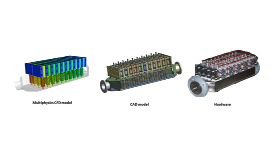
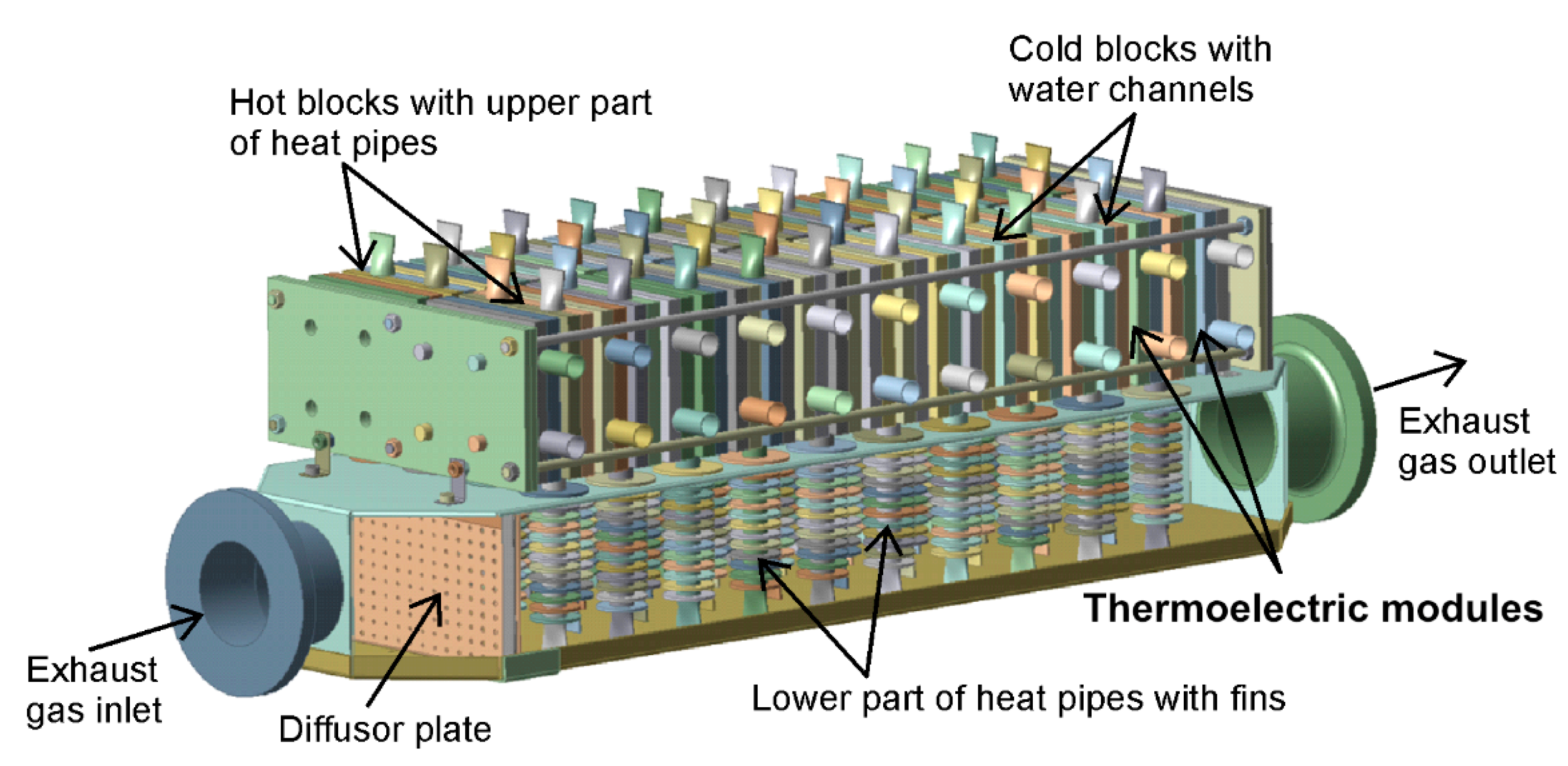
The TEG heat exchanger developed within this work is primarily intended for validation of the new simulation methodology. It consists mainly of two parts as shown in Figure 1. The lower part includes the gas channel where the energy in the hot gas is transported to the upper part—which also includes the thermoelectric modules by use of heat pipes.
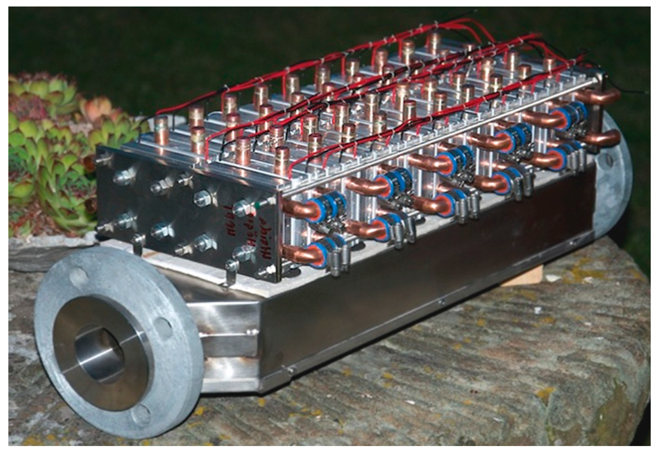
In order to provide a minimum of heat transfer resistance, the heat pipes were made of copper which has excellent thermal conductivity compared to other metals. A corresponding photo of the hardware is shown in Figure 2. For the purpose of achieving a useful voltage level, the 40 modules were connected electrically in five groups in series, each containing 8 modules and the groups were connected together in parallel. In this work, 40 commercial Bi2Te3 modules TEPH1-12680-0.15 from Thermonamics Electronics Co., Ltd. are installed in the TEG heat exchanger. Information about the module efficiency, structure and the electric and thermal properties of the material as function of temperature is provided in the paper by Högblom and Andersson [31] The diffusor plate was designed with increasing size of the holes towards the sides of the plate to partly counteract flow separation and provide uniform heat transfer to the pipes. For the same reason, the heat pipes were design with an increasing number of fins downstream the heat exchanger to provide a uniform heat transfer in the stream wise direction since the gas enthalpy decrease.
The measurements were done in the engine bench laboratory using the exhaust gas from a one cylinder, 2.1-liter diesel engine. Besides engine speed and torque the exhaust gas temperature and flow rate are affected by fuel injection parameters. Three different load points were measured where engine speed and torque were varied resulting in different gas temperatures, mass flow rates and thereby different electrical power generation. During all the experiments the gas temperature, mass flow rate and pressure drop was measured together with the total voltage and current from the TEG unit after sufficiently long time, when steady state conditions was reached. In the following text and figures the three load points are referred to as the low, moderate and high load cases, due to the difference in electrical power generation as shown in the last column in Table 1. The thermoelectric system was connected to an electronic load (Amrel, PLA 1.5K-60-600) where the current and voltage were measured at the different engine load point with an accuracy of 0.05%. Temperatures measurements in thermoelectric heat exchanger were accomplished with a temperature module (National Instruments, CT-120), having a measurements accuracy of 0.05%. Load resistance was chosen to maximize the electrical power output, i.e., load resistance equals the total resistance of the system.
3. Simulation Methodology
The requirements for the multiphysics model developed in this work include models to predicting the rate of turbulent heat transfer and models to predict the thermoelectric power generation and at the same time allow full coupling between the different phenomena. In Figure 1 the front wall of the heat exchanger is removed revealing the interior parts. As shown here the heat transfer from the gas is enhanced by using heat pipes covered by fins. Since the performance of a TEG system is strongly dependent on the temperature difference over the thermoelectric material all thermal resistance from the heat source to the heat sink must be minimized. This can be accomplished by heat pipes, which are sealed tubes containing a gas-liquid mixture that allow large amounts of energy to be transferred with minimal temperature drop by the process of evaporation and condensation. For this purpose, heat pipes have been used together with TEGs applications both at the hot and the cold side [1,20,32,33,34]. Kim et al. and Jang et al. built and analyzed TEG systems containing heat pipes for automotive applications [20,33]. The present heat exchanger contains a total of 22 cold blocks, 20 hot blocks and 40 thermoelectric modules, thereby 2 modules are installed between each cold and hot block. Each hot block is connected to two heat pipes and two thermoelectric modules as shown in Figure 1.
Accurate description of the heat transfer process from the hot gas to the fins in the heat exchanger requires a turbulence model that allows high resolution close to the fins where the thermal boundary layers develops. This means that turbulence models such as the k-ε model with wall functions are not appropriate to use due to the fact that the flow is confined between narrow fins influenced by viscous forces which prevents the use of wall functions as they can only be used when the first grid point is located in the inertial sublayer, i.e., y+ ≥ 30 [35].
For the propose of resolving the turbulent boundary layers and the heat flux correctly the SST k-ω is used. This model is usable all the way through the buffer and viscous sublayers without introducing any turbulence damping function, which is required if a k-ε models should be used in the near wall region [36]. Since the SST k-ω model allows calculation throughout the near wall region including the viscous sublayer, it can resolve regions of different wall stresses thereby allowing the thin thermal boundary layers to be resolved correctly in all parts of the heat exchanger, as long the discretization is dense enough in the wall region. In these simulations the fluid can safely be treated as incompressible gas, using the ideal gas law since the Mach number is approximately 0.1, and the effects due to intramolecular interactions between the molecules are negligible at all temperature and pressure conditions inside the system. The time-filtered continuity equation reads
and the conservation equation for momentum transport, the Reynolds averaged Navier–Stokes equation, is given by
Here the Reynolds stress term, , is closed by the Boussinesq approximation [35], using information about the local turbulent properties, i.e., local length and velocity scales of turbulence, determined by the SST k-ω turbulence model. The SST k-ω model is a two equation turbulence model which allows the advantages of the classical k-ω model (good performance in the near wall region) and k-ε model (for the free stream) to be retained in one and the same model. This makes the SST k-ω model accurate and computationally efficient [36]. In the SST k-ω model, the transport equation for turbulent kinetic energy, k, is given by
and the transport equation for the specific rate of energy dissipation, ω, is given by
Here is the effective diffusivity, P is the production, D is the dissipation of the corresponding variables and is the cross-diffusion term. There are some differences between the classical k-ω model and the SST k-ω, for example in calculation of the production term [36]. The terms describing the production and dissipation of ω as well as the cross-diffusion term also contains a blending function that allows a smooth transition between the k-ω model performance in the near wall regions and the k-ε model performance in the bulk flow. This blending function is determined as a function of the distance to the nearest surface as described by Menter [36]. The energy transport is modeled by
where and the heat diffusivity and is the turbulent Prandtl number. Heat transfer at the boundaries are negligible due to insulation and imposed using zero heat flux boundary conditions in the model, except for boundaries in contact with the thermoelectric modules. Radiative heat transfer between surfaces of different temperature inside the heat exchanger is include in the model. In this work, the discrete ordinates (DO) radiation method is used to solve the radiative transfer equation (RTE) numerically [37] and a transport equation is solved for the radiation intensity in the spatial coordinates,
Here the radiation absorption coefficient for the gas is calculated used weighted-sum-of-gray-gases (WSGG) model [37].
Besides Fourier heat conduction to the thermoelectric modules, the effect of Peltier, Thomson and Joule heating in the semiconducting material needs to be accounted for in the CFD model. The complexity of this modelling is twofold. Firstly, it is largely affected by the current in the semiconducting material which implies that it is also affected by the electrical circuit i.e., electric connections between the different thermoelectric modules in the system. Secondly the Peltier, Thomson and Joule heating effects the local temperature and the heat flux in the system causing effects on heat transfer over the entire system that should be handled by the CFD model, expect in the case for open circuit but that is of no interest for heat recovery systems. Consequently, the problem requires two way coupling between the CFD and thermoelectric models allowing the effect of current and heat transfer over the entire heat exchanger to be included in the analysis. The generic formulation of the thermoelectric models consists of three sub models. This includes electrical and thermal models for the individual modules and one model for the circuit of the connected system. Derivation, discussion and validation of these models, over a wide range of operating conditions, even when some of the modules in the network work with reversed current, is found in [30]. The electrical model contains modification to the electrical model proposed by Montecuccu et al. [38], which for individual modules in the network is given by
In Equation (7) the Seebeck voltage and the internal resistivity is accounted for, the latter is affected by both the electrical contact resistances in material junctions and the materials resistivity. In Equation (7), U and I is the voltage over and current through the module, respectively, and are the average temperature in the semiconducting material and the temperature difference between the hot and the cold blocks adjacent to the module. Here coefficients are regression parameters determined for the module using the method described in [30]. Furthermore, the heat flow on the cold side of the for individual modules are given by
The total heat flow in Equation (8), is described by Fourier heat conduction along with the Peltier and Thomson effect and the Joule heating. In contrast the heat flow on the hot side of the modules also contains an additional term for the heat that is converted to electrical energy
As a result, the difference between the heat flow to the module surface on the hot side and from the module surface on the cold side corresponds to the net electric power generated by the thermoelectric modules. A general circuit model for the connected system based on Ohms law and Kirchhoff’s current law is presented in [30]. In this case the thermoelectric generator used for validation has 40 modules (8×5) and the equations becomes
and
where index, i, represent the 5 different serial connected groups and index, j, represent the each of the 8 modules within the groups. By solving of Equations (1)–(11) a two-way coupled energy transport is made possible by using the thermoelectric models as subgrid models in CFD analysis and by assigning heat flow boundary conditions on the thermoelectric module surfaces in the CFD model.
A block diagram describing the coupling and how the thermoelectric models are implemented in the CFD analysis is shown in Figure 3. As shown here the temperature distribution over the different modules effect the electrical performance. This is in turn affected by the module current which is predicted by the circuit model. Knowledge of the current distribution allows Peltier, Thomson and Joule effects to be quantified when passing back information on the heat flow to the CFD solver. Hence, the circuit model allows local variations in driving force to be sensed throughout the entire system of thermoelectric modules. The flow of hot gases and the turbulent heat transfer were modeled using commercial CFD solver—Ansys Fluent 19—and the three thermoelectric models are implemented in the CFD analysis as subgrid programs written in C. Every iteration, the temperature inside the hot and cold blocks adjacent to all the modules are calculated by the program and the Seebeck voltages and internal resistances are calculated in the electrical model. Together with the load resistance and the electrical connections the currents through all modules are determined in an iterative manner in the circuit model and the electrical model pass on information allowing the thermal effects to be calculated by the thermal model, Equations (7) and (8). This information is passed back to the CFD solver to be used as heat flux boundary condition in the next iteration as shown in Figure 3. Thereby the effect of current on the heat flow in the CFD analysis is accounted for throughout the entire heat exchanger, providing a full two-way coupling through energy conservation.
In other words, by allowing the flow field and temperature fields to be solved simultaneously with the thermoelectric power generation—and by accounting for the Peltier, Thomson and Joule effects—the multiphysics model presented here provides an efficient and correct modeling approach to handle an arbitrary number of thermoelectric modules in CFD analysis in a physical and robust way.
3.1. Mesh Structure, Numeric Methods and Sensitivity Analysis
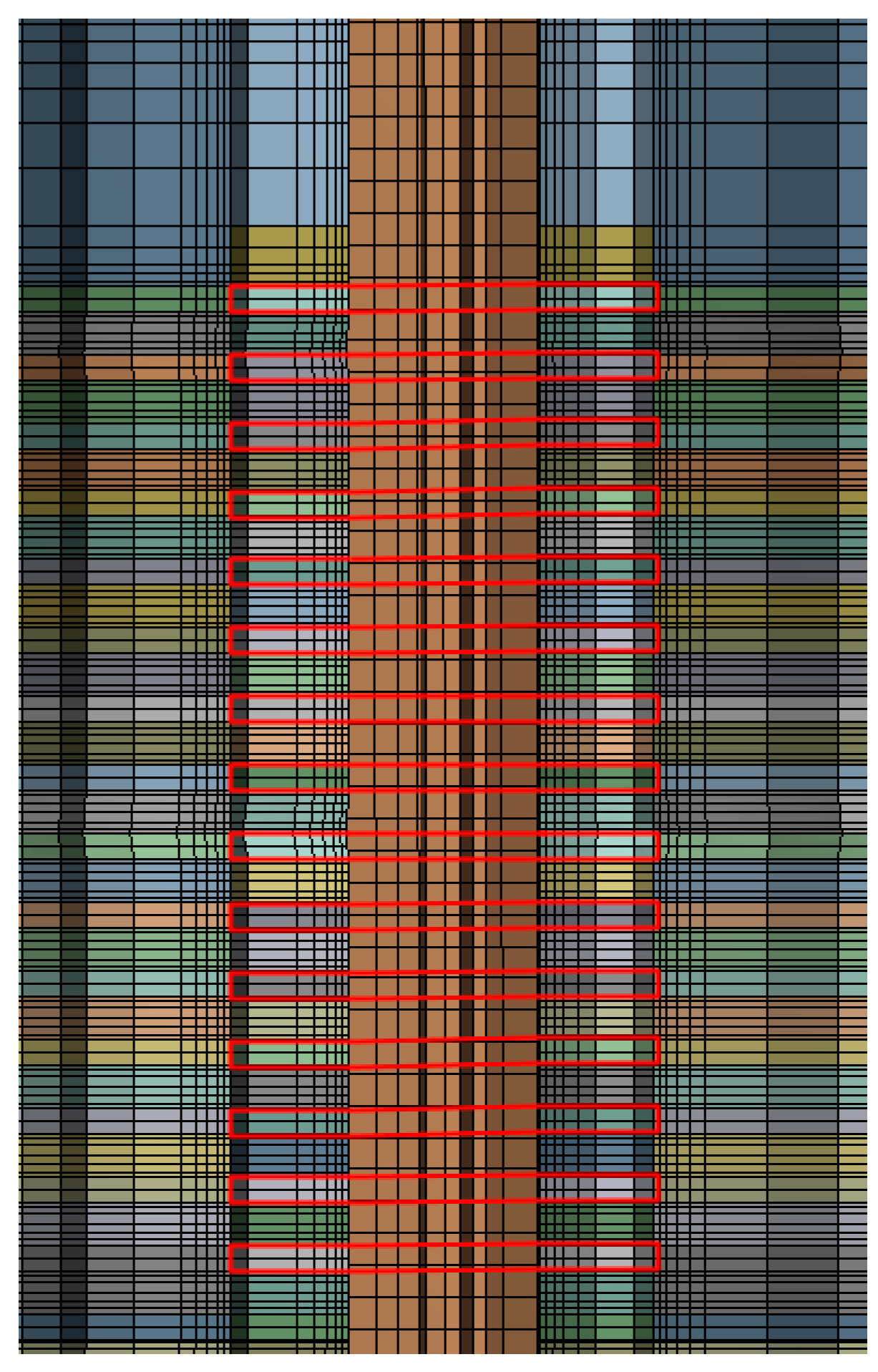
High quality heat-transfer simulations require good mesh quality and suitable numeric schemes to control numeric errors. For this purpose, prism layers were introduced in all boundary layers and second–order discretization schemes were used to minimize numeric errors. Since the geometry of the computational domain is complex, the geometry was divided into different zones allowing generation of a swept mesh and high-quality hexahedral cells as depicted in Figure 4.
Mesh independence was confirmed by evaluating the solution variables using models with different mesh resolution. The mesh adaption was done by refining mesh zones with large gradients of the solution variables. Both turbulent kinetic energy and the thermal field have the largest gradients in the near wall regions which is consistent with the main heat transfer resistance being in the gas film close to the surfaces. Evaluation of mesh independence showed that mesh independent results were obtained with a model containing 4.2 million cells. This mesh was therefore used for all the simulations in this study. Simulations were done on a computer cluster using up to 128 cores.
Furthermore, a sensitivity analysis with respect to the turbulence model was done. The SST k-ω turbulence model is judged the best model in this case, due to the reasons discussed earlier, but turbulence simulations using dedicated low Reynolds k-ε models can also give good results. Similar to the SST k-ω this model also allows integration throughout the near wall region. This is achieved by using turbulence dampening functions that are active in the buffer and viscous sublayers. In this case the Launder-Sharma low Reynolds k-ε model was used [39]. For both SST k-ω and Launder-Sharma models the y+ -value were sufficiently low on all interior walls. It was found the difference between the turbulence models is not critical since the difference was very small, lower than 1% for the predicted pressure drop and heat transfer rates. Finally, a sensitivity analysis was made with respect to the turbulence boundary conditions as discussed in the section below.
3.2. Boundary Conditions and Material Data
The boundary condition given in Table 1, are specified according to the mass flow rates obtained at the different engine load cases. Turbulence boundary conditions at the inlet were given as turbulent intensity and the turbulent length scale. These properties were determined based on best practice guidelines, i.e., turbulence intensity was estimated as and the length scale as 7% of the hydraulic diameter [35]. A sensitivity analysis of the turbulence boundary conditions was done by changing these values by 10%. It was found the boundary conditions had no significant effect on the final results (<0.1%). These results can be understood better by analyzing the rate of turbulence dissipation and turbulence production. The analysis revealed turbulence in the inlet does not survive long enough to have any impact after the diffusor plate, shown in Figure 1. At the diffusor plate new turbulence is continuously generated which dominate the rate of momentum and heat transfer downstream in the system, thereby making the simulations less sensitive to the turbulent boundary conditions applied at the inlet. At the exhaust gas outlet, a constant pressure boundary condition was implemented. The walls of the well-insulated heat exchanger were treated adiabatically using a zero heat flux boundary condition.
The temperature dependency of the specific heat, viscosity and thermal conductivity of the gas were given by NIST data. Analysis of the heat transfer rate through the heat pipes shows that this is not a limiting factor for the overall heat transfer rate from the exhaust gas bulk to the surface of the hot block, instead the main heat transfer resistance lies in the gas film. This allows, the heat transfer in the heat pipes to be simulated using an effective heat conductivity. The same modeling strategy for heat pipes has been presented in the literature and shown to give accurate results [40]. This was also validated by measurements of heat flow in heat pipes for the temperatures relevant for the system, which shows all conditions are far from being controlled by the internal heat transfer rate inside the heat pipes. To finally close the model, there are thermal contact resistances present between the heat pipes and the hot aluminum blocks and between the heat pipes and the fins, which are accounted for in these simulations. The contact resistances specified in these simulations were determined in a previous study for similar material contacts [31], which is consistent with values reported in the literature [41].
4. Results and Discussion
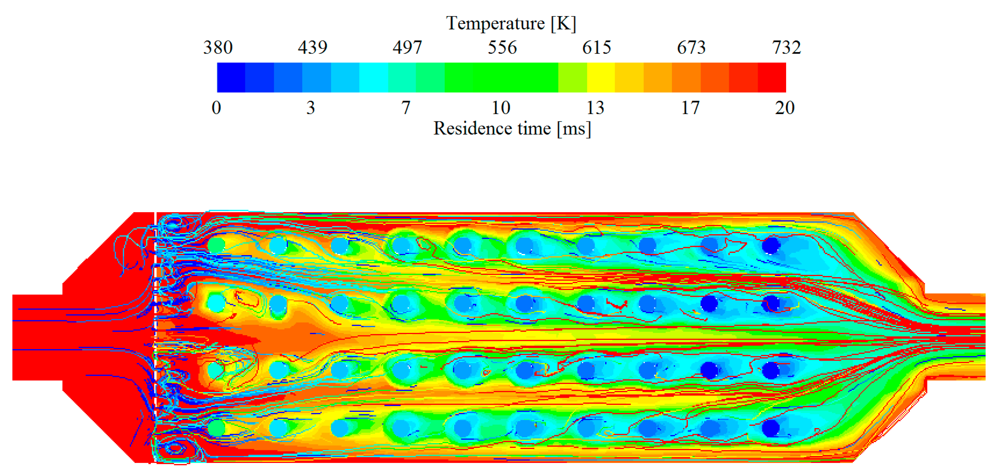
The results presented here are based on mesh independent simulations using the SST k-ω model for the three engine load points introduced earlier. Validation of the simulation model includes both the fluid dynamics and the thermoelectric performance obtained by solving Equations (1)–(11). The simulations were run on a computer cluster until convergence of all solution variables and by ensuring mass and energy conservation at the end of the iterations. Figure 5 shows the temperature field inside the heat exchanger in a horizontal plane in the middle section overlaid with streamlines colored by the residence time. The heat transfer to the heat pipes and the thermoelectric modules causes the temperature to decrease in the exhaust gas flow, mainly in the center whereas the flow along the outermost streamlines are less affected. Due to insulation at the walls the gas temperature in the wall region only decrease as a result of turbulent mixing with the bulk fluid that has lower temperature. When analyzing the temperature distribution at the outlet in Figure 5, it becomes clear that the gas is not fully mixed, i.e., hot gas flows along the pipe walls and cold gas in the center. Therefore, temperature measurements at this location can be sensitive to the location of the sensor. Contrary, pressure measurements would not be sensitive since radial variations in pressure is not significant. From an energy balance point of view approximately one third of the enthalpy is transferred to the modules. Out of this energy a fraction is converted to electric energy in the thermoelectric modules.
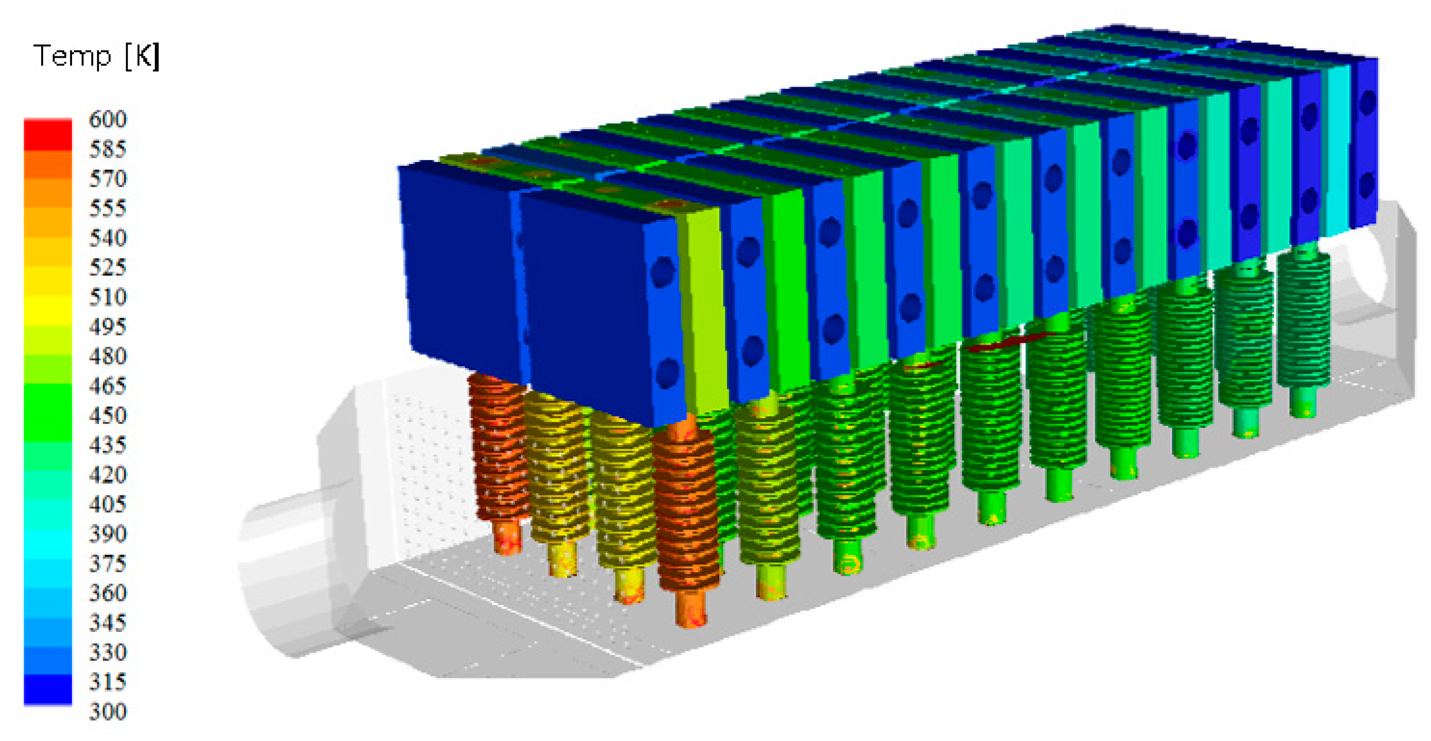
The temperature distribution also results in differences in local heat transfer rates and thereby a distribution of surface temperatures between the hot aluminum blocks. Figure 6 displays the temperature distribution on the heat pipe surfaces and the temperature of the hot and cold aluminum blocks, respectively. Here the effect of the inlet diffuser plate on heat transfer is clearly visible. The temperature difference between the first and second row of heat pipes is much larger compared to the following rows. This is explained by that the turbulent jets formed by the diffuser plate does not penetrate long enough to have significant effect beyond the second row of heat pipes. It is also noticeable how the diffuser plate, which is designed with smaller holes in the middle part and larger holes at the sides actually provides higher heat transfer rate to the outermost heat pipes, which are 40 °C warmer compared to the two heat pipes in the center. However, this difference is not fully sensed by the thermoelectric modules, since the metal blocks to which modules are attached, have high thermal diffusivity that allows lateral heat flow which minimize the temperature distribution over the module surfaces. To counteract the problem with low heat transfer rate in gases and simultaneously provide more homogenous thermal load on the thermoelectric modules, the heat pipes are designed with gradually increasing number of fins. As shown in Figure 6, the first three rows of heat pipes at the inlet have 13 fins each, the next three rows have 16 fins and the last four rows are designed with 20 fins each to compensate for the temperature drop in the stream wise direction. The simulations reveal that the present design does not entirely compensate for this and the model provide detailed enough information to allow optimization of the design.
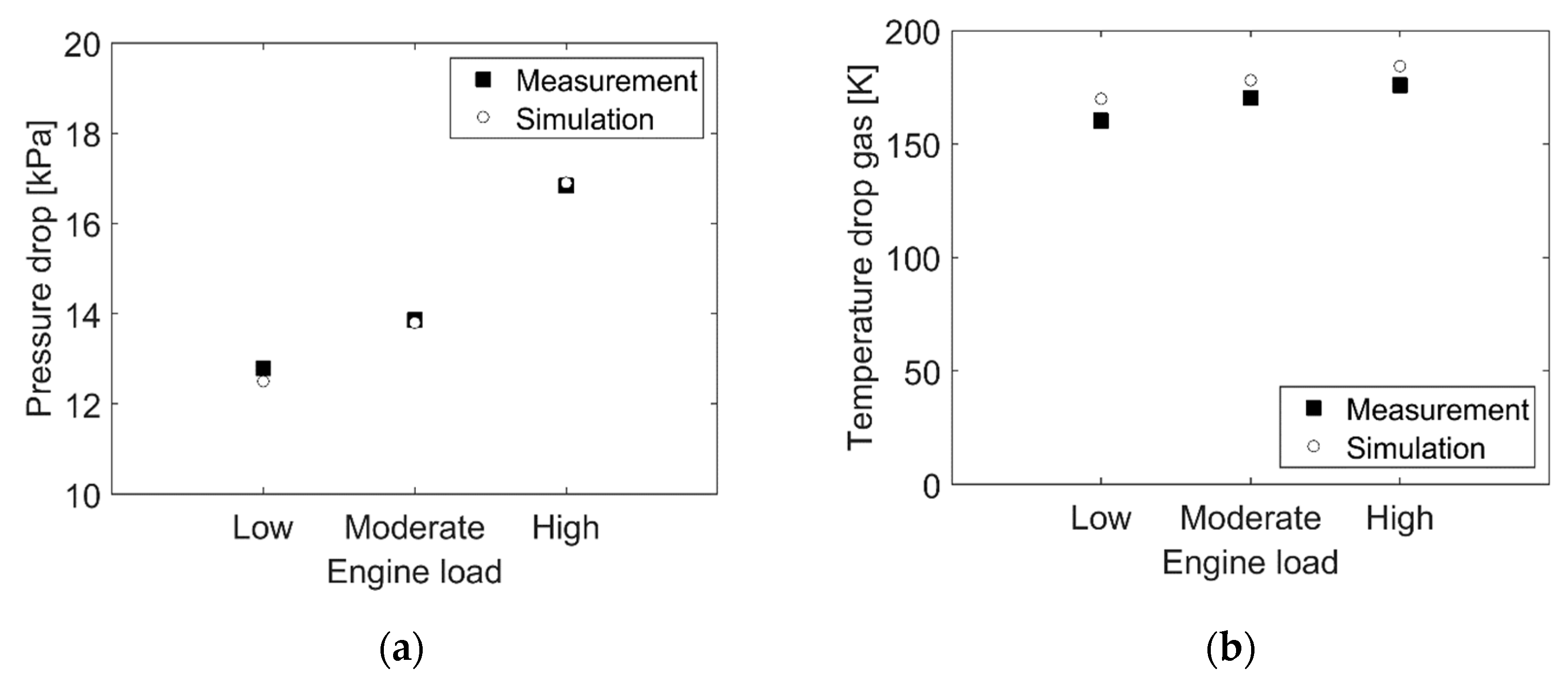
Validation of pressure drop and temperature drop for the three engine load points at steady state engine bench conditions is summarized in Figure 7. Overall, the simulation results agree very well at the three engine loads points. Considering the calculated pressure drop over the thermoelectric heat exchanger the error is only 2.3%, 0.4% and 0.4% for the different engine loads, as shown in Figure 7a. Figure 7b shows the temperature drop, defined as the difference between the inlet and outlet exhaust gas temperature. Predictions of the temperature drop is considered good, but slightly larger, 6.0%, 4.6% and 4.8% in the three cases. Considering the complexity of the geometry and that the flow contains bot turbulence and regions affected by viscous forces including turbulent jets at the diffusor plate this is considered as very good results. As shown Figure 7b, there is small and systematic deviation that can be due to that a thermocouple installed in the gas flow may register a slightly too high gas temperature since the sensor is influenced by radiation from the hot surrounding wall. The sensor is installed in the center of the pipe where the temperature is lower compared to the surrounding wall. If a slightly too high temperature is measured by the sensor at the outlet it follows that the temperature drop over the system gets too small. Consequently, measurement points, in Figure 7b, will be lower than they should. Calculation accounting for both convective heat transfer and radiative heat transfer to the thermocouple indicates that half the difference seen in Figure 7b can be explained by this effect. In other words, half the difference shown in Figure 7b can be explained by this phenomenon. The accuracy of the predications is therefore closer to 3% rather than 6% as seen at first. The use of radiation shielded thermocouples, can solve this problem or an approach using the two-thermocouple method can be used to minimize the difference [42].
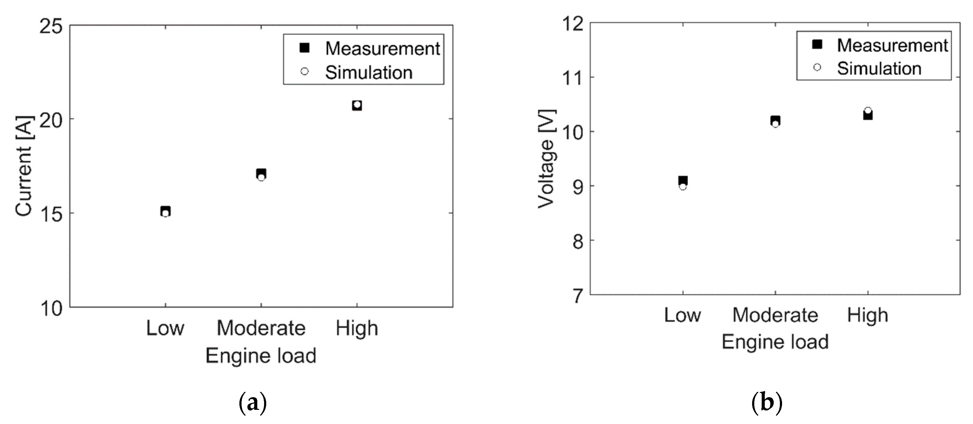
In order to evaluate the accuracy of the predicted electric power generation, the current and voltage are compared with measurements at the three load points. Figure 8a,b summarizes the results for the thermoelectric power generation and shows that the predicted current and voltage agrees very well with the measurements for all engine loads. The error is less than 1.5% for all experimental conditions and no systematic error exists.
Overall, the agreement between the simulation results and measurements is good. This leads to the conclusion that the multiphysics CFD model accounts correctly for both fluid dynamics, including pressure drop and heat transfer and the thermoelectric power generation. At the same time, it means that multiphysics model allows the importance of two way coupling to be analyzed and understood particularly since the thermoelectric modules operate at different temperature while being electrically connected. The temperature distribution obtained in these simulations were therefore used to analyze a case where all modules are allowed to operate individually at the current maximizing their power output to assess the impact on the electrical power output of the TEG system. This gives an estimate of the highest power output achievable at these thermal conditions and provides a direct measure of the magnitude of the non-ideal effect caused by the electrical connection and consequently also the error that is introduced if the two way coupling is neglected in evaluation of the TEG performance. Considering the three engine load cases such simulation approach leads to overprediction of the power output corresponding to 5.4%, 5.2% and 4.6%, respectively. These are significant deviations compared to the accuracy achieved with the proposed model which gives less than 1.5% difference.
The error introduced by simplistic analysis could obviously be much larger when the temperature distribution is more significant which is expected from systems working at higher heat recovery levels. An improved heat exchanger design that allows more energy to be transfer from the gas results in a larger temperature difference among the thermoelectric modules and thereby also larger difference in heat flow and Seebeck voltage in the different modules. Consequently, the non-ideal effects would increase substantially. In order to understand this effect better at higher heat recovery level the system was simulated with increased heat transfer. The results are summarized below in Table 2.
As shown in Table 2, the difference between the optimal (fictious) power and the real power generation increase rapidly in a system of connected modules with increasing heat recovery level. This is due to the electrical connection between the modules inside the thermoelectric generator and increasing temperature differences in the system. A simplistic modeling approach would therefor lead to unnecessary large simulation error which highlights the importance of using a coupled approach in simulating the heat transfer and thermoelectric power generation. Considering that the methodology presented here is computational efficient and generic it may allow accurate prediction of power generation in other systems and concepts by accounting for effect of the current on the heat flow throughout the systems.
5. Conclusions
A multiphysics simulation methodology was developed and validated that permits the extension of computational fluid dynamics (CFD) simulations to account for electric power generation and its effect on the energy transport, the Seebeck voltage, the electrical currents in thermoelectric systems. The energy transport through Fourier, Peltier, Thomson and Joule mechanisms as function of temperature and electrical current—and the electrical connection between thermoelectric modules—was integrated in the CFD analysis by subgrid models. Thereby the effect of current on the heat flow in the CFD analysis is accounted for throughout the entire heat exchanger, providing a full two-way coupling through energy conservation. The accuracy was evaluated for a thermoelectric generator containing 40 connected thermoelectric modules in engine bench laboratory and showed that the fluid dynamics and the thermoelectric performance were predicted very well. Comparison with simulation results showed the predicted pressure drop has an error of 2.3%, while the temperature drop over system has an error of 3.0%, at all experimental conditions studied, when accounting for the radiative effects on the thermocouple. The thermoelectric power generation was predicted with high accuracy and the error in voltage and current was less than 1.5% at the exhaust gas flow rates and temperatures studied. Simulation results confirm computational efficiency and stable simulations with low increase in computational time compared to standard CFD heat-transfer simulations. Furthermore, the importance of two way coupling of energy transport was analyzed. Evidence was found that even at the lowest heat transfer rate studied it is required to use a full two way coupling in the energy transport to accurately predict the electric power generation.
Author Contributions
Methodology O.H., R.A.; simulations O.H.; validation, O.H., R.A; writing, O.H., R.A.; project administration R.A.; funding acquisition, R.A. All authors have read and agreed to the published version of the manuscript.
Funding
This work was supported by the Swedish Foundation for Strategic Environmental Research.
Acknowledgments
The financial support from the Swedish Foundation for Strategic Environmental Research is gratefully acknowledged. The authors would like to thank Termo-Gen AB building the prototype and Volvo Technology AB for doing the engine bench measurements. The multiphysics simulations were done using the high-performance computer cluster at Chalmers University of Technology, supported by the Swedish National Infrastructure for Computing, SNIC.
Conflicts of Interest
The authors declare no conflict of interest.
Nomenclature
| Seebeck coefficient, V K−1 | |
| cp | Heat capacity, J kg−1 K−1 |
| ε | Dissipation rate of turbulent kinetic energy, m2 s−3 |
| Current, A | |
| I | Radiation intensity, J m−2 s−1 |
| k | Turbulent kinetic energy, m2 s−2 |
| λ | Heat conductivity, W m−1 K−1 |
| µ | Dynamic viscosity, Pa s |
| ν | Kinematic viscosity, m2 s−1 |
| Peltier coefficient, V | |
| Combined Peltier and Thomson coefficients, V | |
| P | Pressure, Pa |
| Q | Source term, W m−3 |
| Heat flow, W | |
| ρ | Density, kg m−3 |
| Resistance, Ω | |
| Temperature, K | |
| Thomson coefficient, V K−1 | |
| Voltage, V | |
| Velocity, m s−1 | |
| ω | Specific dissipation rate of turbulent kinetic energy, s−1 |
| y+ | Dimensionless wall distance, - |
Subscripts
| Average between hot and cold side | |
| Cold side | |
| Hot side | |
| Internal | |
| L | Load |
| Si | Seebeck where i = 1, 2 |
| Ri | Internal resistance |
| Fi | Fourier conduction |
| PTi | Peltier & Thomson |
| T | Turbulent |
References
- He, W.; Su, Y.; Riffat, S.; Hou, J.; Ji, J. Parametrical analysis of the design and performance of a solar heat pipe thermoelectric generator unit. Appl. Energy 2011, 88, 5083–5089. [Google Scholar] [CrossRef]
- Ji, J.; Lu, J.-P.; Chow, T.-T.; He, W.; Pei, G. A sensitivity study of a hybrid photovoltaic/thermal water-heating system with natural circulation. Appl. Energy 2007, 84, 222–237. [Google Scholar] [CrossRef]
- Zhang, M.; Miao, L.; Kang, Y.P.; Tanemura, S.; Fisher, C.A.J.; Xu, G.; Li, C.X.; Fan, G.Z. Efficient, low-cost solar thermoelectric cogenerators comprising evacuated tubular solar collectors and thermoelectric modules. Appl. Energy 2013, 109, 51–59. [Google Scholar] [CrossRef]
- Suter, C.; Jovanovic, Z.R.; Steinfeld, A. 1 kWe thermoelectric stack for geothermal power generation—Modeling and geometrical optimization. Appl. Energy 2012, 99, 379–385. [Google Scholar] [CrossRef]
- Whalen, S.A.; Dykhuizen, R.C. Thermoelectric energy harvesting from diurnal heat flow in the upper soil layer. Energy Convers. Manag. 2012, 64, 397–402. [Google Scholar] [CrossRef]
- Espinosa, N.; Lazard, M.; Aixala, L.; Scherrer, H. Modeling a Thermoelectric Generator Applied to Diesel Automotive Heat Recovery. J. Electron. Mater. 2010, 39, 1446–1455. [Google Scholar] [CrossRef]
- Högblom, O.; Andersson, R. CFD Modeling of Thermoelectric Generators in Automotive EGR-coolers American Institute of Physics. Conf. Ser. 2011, 1449, 497–500. [Google Scholar]
- Wang, Y.; Dai, C.; Wang, S. Theoretical analysis of a thermoelectric generator using exhaust gas of vehicles as heat source. Appl. Energy 2013, 112, 1171–1180. [Google Scholar] [CrossRef]
- Li, B.; Huang, K.; Yan, Y.; Li, Y.; Twaha, S.; Zhu, J. Heat transfer enhancement of a modularised thermoelectric power generator for passenger vehicles. Appl. Energy 2017, 205, 868–879. [Google Scholar] [CrossRef]
- Nonthakarn, P.; Ekpanyapong, M.; Nontakaew, U.; Bohez, E.L.J. Design and Optimization of an Integrated Turbo-Generator and Thermoelectric Generator for Vehicle Exhaust Electrical Energy Recovery. Energies 2019, 12, 3134. [Google Scholar] [CrossRef] [Green Version]
- El-Genk, M.S.; Saber, H.H. Performance analysis of cascaded thermoelectric converters for advanced radioisotope power systems. Energy Convers. Manag. 2005, 46, 1083–1105. [Google Scholar] [CrossRef]
- Cho, Y.H.; Park, J.; Chang, N.; Kim, J. Comparison of Cooling Methods for a Thermoelectric Generator with Forced Convection. Energies 2020, 13, 3185. [Google Scholar] [CrossRef]
- In, B.D.; Lee, K.H. A study of a thermoelectric generator applied to a diesel engine. Proc. Inst. Mech. Eng. Part. D J. Automob. Eng. 2015, 230, 133–143. [Google Scholar] [CrossRef] [Green Version]
- Liu, X.; Deng, Y.; Li, Z.; Su, C. Performance analysis of a waste heat recovery thermoelectric generation system for automotive application. Energy Convers. Manag. 2015, 90, 121–127. [Google Scholar] [CrossRef]
- Liu, X.; Li, C.; Deng, Y.; Su, C. An energy-harvesting system using thermoelectric power generation for automotive application. Int. J. Electr. Power Energy Syst. 2015, 67, 510–516. [Google Scholar] [CrossRef]
- Tang, Z.B.; Deng, Y.D.; Su, C.Q.; Shuai, W.W.; Xie, C.J. A research on thermoelectric generator’s electrical performance under temperature mismatch conditions for automotive waste heat recovery system. Case Stud. Therm. Eng. 2015, 5, 143–150. [Google Scholar] [CrossRef] [Green Version]
- Thacher, E.F.; Helenbrook, B.T.; Karri, M.A.; Richter, C.J. Testing of an automobile exhaust thermoelectric generator in a light truck. Proc. Inst. Mech. Eng. Part. D J. Automob. Eng. 2007, 221, 95–107. [Google Scholar] [CrossRef]
- Hsu, C.-T.; Huang, G.-Y.; Chu, H.-S.; Yu, B.; Yao, D.-J. Experiments and simulations on low-temperature waste heat harvesting system by thermoelectric power generators. Appl. Energy 2011, 88, 1291–1297. [Google Scholar] [CrossRef]
- Hsu, C.-T.; Yao, D.-J.; Ye, K.-J.; Yu, B. Renewable energy of waste heat recovery system for automobiles. J. Renew. Sustain. Energy 2010, 2, 13105. [Google Scholar] [CrossRef]
- Kim, S.-K.; Won, B.-C.; Rhi, S.-H.; Kim, S.-H.; Yoo, J.-H.; Jang, J.-C. Thermoelectric Power Generation System for Future Hybrid Vehicles Using Hot Exhaust Gas. J. Electron. Mater. 2011, 40, 778–783. [Google Scholar] [CrossRef]
- Antonova, E.; Looman, D. Finite elements for thermoelectric device analysis in ANSYS. In Proceedings of the ICT 2005 24th International Conference on Thermoelectrics, Institute of Electrical and Electronics Engineers (IEEE), Clemson, SC, USA, 19–23 June 2005; pp. 215–218. [Google Scholar]
- Rezaniakolaie, A.; Rosendahl, L. A comparison of micro-structured flat-plate and cross-cut heat sinks for thermoelectric generation application. Energy Convers. Manag. 2015, 101, 730–737. [Google Scholar] [CrossRef]
- Weng, C.-C.; Huang, M.-J. A simulation study of automotive waste heat recovery using a thermoelectric power generator. Int. J. Therm. Sci. 2013, 71, 302–309. [Google Scholar] [CrossRef]
- Martinez, A.; Vián, J.G.; Astrain, D.; Rodriguez, A.; Berrio, I. Optimization of the Heat Exchangers of a Thermoelectric Generation System. J. Electron. Mater. 2010, 39, 1463–1468. [Google Scholar] [CrossRef]
- Tang, Z.B.; Deng, Y.D.; Su, C.Q.; Yuan, X.H. Fluid Analysis and Improved Structure of an ATEG Heat Exchanger Based on Computational Fluid Dynamics. J. Electron. Mater. 2014, 44, 1554–1561. [Google Scholar] [CrossRef]
- Su, C.Q.; Xu, M.; Wang, W.S.; Deng, Y.D.; Liu, X.; Tang, Z.B. Optimization of Cooling Unit Design for Automotive Exhaust-Based Thermoelectric Generators. J. Electron. Mater. 2015, 44, 1876–1883. [Google Scholar] [CrossRef]
- Wang, Y.; Wu, C.; Tang, Z.-B.; Yang, X.; Deng, Y.; Su, C. Optimization of Fin Distribution to Improve the Temperature Uniformity of a Heat Exchanger in a Thermoelectric Generator. J. Electron. Mater. 2014, 44, 1724–1732. [Google Scholar] [CrossRef]
- Deng, Y.D.; Zhang, Y.; Su, C.Q. Modular Analysis of Automobile Exhaust Thermoelectric Power Generation System. J. Electron. Mater. 2014, 44, 1491–1497. [Google Scholar] [CrossRef]
- Yu, S.; Du, Q.; Diao, H.; Shu, G.; Jiao, K. Start-up modes of thermoelectric generator based on vehicle exhaust waste heat recovery. Appl. Energy 2015, 138, 276–290. [Google Scholar] [CrossRef]
- Högblom, O.; Andersson, R. A simulation framework for prediction of thermoelectric generator system performance. Appl. Energy 2016, 180, 472–482. [Google Scholar] [CrossRef]
- Högblom, O.; Andersson, R. Analysis of Thermoelectric Generator Performance by Use of Simulations and Experiments. J. Electron. Mater. 2014, 43, 2247–2254. [Google Scholar] [CrossRef] [Green Version]
- Aranguren, P.; Astrain, D.; Rodriguez, A.; Martinez, A. Experimental investigation of the applicability of a thermoelectric generator to recover waste heat from a combustion chamber. Appl. Energy 2015, 152, 121–130. [Google Scholar] [CrossRef] [Green Version]
- Jang, J.-C.; Chi, R.-G.; Rhi, S.-H.; Lee, K.-B.; Hwang, H.-C.; Lee, J.-S.; Lee, W.-H. Heat Pipe-Assisted Thermoelectric Power Generation Technology for Waste Heat Recovery. J. Electron. Mater. 2015, 44, 2039–2047. [Google Scholar] [CrossRef]
- He, W.; Su, Y.; Wang, Y.; Riffat, S.; Ji, J. A study on incorporation of thermoelectric modules with evacuated-tube heat-pipe solar collectors. Renew. Energy 2012, 37, 142–149. [Google Scholar] [CrossRef]
- Andersson, B.; Andersson, R.; Håkansson, L.; Mortensen, M.; Sudiyo, R.; van Wachem, B.G.M. Computational Fluid Dynamics for Engineers; Cambridge University Press: Cambridge, UK, 2011. [Google Scholar]
- Menter, F.R. Two-equation eddy-viscosity turbulence models for engineering applications. AIAA J. 1994, 32, 1598–1605. [Google Scholar] [CrossRef] [Green Version]
- Modest, M.F. Radiative Heat Transfer; Elsevier BV: Amsterdam, The Netherlands, 2003. [Google Scholar]
- Montecucco, A.; Siviter, J.; Knox, A.R. The effect of temperature mismatch on thermoelectric generators electrically connected in series and parallel. Appl. Energy 2014, 123, 47–54. [Google Scholar] [CrossRef] [Green Version]
- Launder, B.E.; Sharma, B.I. Application of the energy-dissipation model of turbulence to the calculation of flow near a spinning disc. Lett. Heat Mass Transf. 1974, 1, 131–137. [Google Scholar] [CrossRef]
- Thayer, J. Analysis of a heat pipe assisted heat sink. In Proceedings of the 9th International FLOTHERM Users Conference, Orlando, FL, USA, 18–19 October 2000. [Google Scholar]
- Chung, D. Materials for thermal conduction. Appl. Therm. Eng. 2001, 21, 1593–1605. [Google Scholar] [CrossRef]
- Brohez, S.; Delvosalle, C.; Marlair, G. A two-thermocouples probe for radiation corrections of measured temperatures in compartment fires. Fire Saf. J. 2004, 39, 399–411. [Google Scholar] [CrossRef]
Figure 1.
Design of the thermoelectric generator (TEG) heat exchanger.

Figure 2.
Photo of the TEG heat exchanger hardware.

Figure 3.
Schematic of program structure and calculation procedure.

Figure 4.
Cross section of the computational mesh through one of the heat pipes.

Figure 5.
Streamlines and temperature distribution in a horizontal plane at moderate engine load.

Figure 6.
Temperature distribution on heat pipe surfaces and aluminum blocks, high-engine-load case.
Figure 6.
Temperature distribution on heat pipe surfaces and aluminum blocks, high-engine-load case.

Figure 7.
Comparison between experiments and simulation results. (a) Pressure drop; (b) temperature drop.
Figure 7.
Comparison between experiments and simulation results. (a) Pressure drop; (b) temperature drop.

Figure 8.
Comparison between experiments and simulation results. (a) Current; (b) voltage.


Table 1.
Engine bench load points used for model validation.
| Load Point | Mass Flow (g/s) | Gas Temp., Inlet (C) | Electric Power (W) |
|---|---|---|---|
| Low | 78.56 | 423.1 | 137.1 |
| Moderate | 79.99 | 459.2 | 174.7 |
| High | 88.01 | 489.4 | 212.6 |
Table 2.
Electrical power output as function of heat recovery level.
| Transferred Energy (%) | Real Power (W) | Optimal Power (W) | Difference (%) |
|---|---|---|---|
| 34.0% | 136.2 | 142.5 | 4.6 |
| 56.0% | 335.8 | 379.6 | 13.0 |
© 2020 by the authors. Licensee MDPI, Basel, Switzerland. This article is an open access article distributed under the terms and conditions of the Creative Commons Attribution (CC BY) license (http://creativecommons.org/licenses/by/4.0/).
Share and Cite
MDPI and ACS Style
Högblom, O.; Andersson, R. Multiphysics CFD Simulation for Design and Analysis of Thermoelectric Power Generation. Energies 2020, 13, 4344. https://doi.org/10.3390/en13174344
AMA Style
Högblom O, Andersson R. Multiphysics CFD Simulation for Design and Analysis of Thermoelectric Power Generation. Energies. 2020; 13(17):4344. https://doi.org/10.3390/en13174344
Chicago/Turabian StyleHögblom, Olle, and Ronnie Andersson. 2020. "Multiphysics CFD Simulation for Design and Analysis of Thermoelectric Power Generation" Energies 13, no. 17: 4344. https://doi.org/10.3390/en13174344
Note that from the first issue of 2016, this journal uses article numbers instead of page numbers. See further details here.