Location and Sizing of Micro-Grids to Improve Continuity of Supply in Radial Distribution Networks


Institute for Research in Technology (IIT), Comillas Pontifical University, 28015 Madrid, Spain
*
Author to whom correspondence should be addressed.
Energies 2020, 13(13), 3495; https://doi.org/10.3390/en13133495
Submission received: 19 May 2020
/
Revised: 18 June 2020
/
Accepted: 1 July 2020
/
Published: 6 July 2020
(This article belongs to the Special Issue Integration of Renewable and Distributed Energy Resources in Power Systems)
Abstract
:The steady decline in the prices of distributed energy resources (DERs), such as distributed renewable generation and storage systems, together with more sophisticated monitoring and control strategies allow power distribution companies to enhance the performance of the distribution network, for instance improving voltage control, congestion management, or reliability. The latter will be the subject of this paper. This paper addresses the improvement of continuity of supply in radial distribution grids in rural areas, where traditional reinforcements cannot be carried out because they are located in secluded areas or in naturally protected zones, where the permits to build new lines are difficult to obtain. When a contingency occurs in such a feeder, protection systems isolate it, and all downstream users suffer an interruption until the service is restored. This paper proposes a novel methodology to determine the optimal location and size of micro-grid systems (MGs) used to reduce non-served energy, considering reliability and investment costs. The proposed model additionally determines the most suitable combination of DER technologies. The resulting set of MGs would be used to supply consumers located in the isolated area while the upstream fault is being repaired. The proposed methodology is validated through its application to a case study of an actual rural feeder which suffers from reliability issues due to the difficulties in obtaining the necessary permissions to undertake conventional grid reinforcements.
1. Introduction
The digitalization of the energy industry represents a turning point in the sector development [1]. In the case of electricity network planning [2], until the end of the 20th century, networks were mainly composed of a set of passive assets governed by electromechanical protection elements. With the sector digitalization, a wide range of possibilities enabling an increase in global social welfare has been opened. Regarding system planning and operation, these possibilities are translated into new management strategies that allow optimizing the performance of the system.
Nowadays, the levels of monitoring and control of transmission grids are fairly high; however, transmission only accounts for 3% of the total length of the European electricity network [3]. The remaining 97% corresponds to the distribution system [4], whose monitoring levels are significantly lower, especially in the case of rural networks [5]. These grids are mostly radial. Consequently, a failure in any of the network elements usually implies the loss of supply for all customers located downstream of the nearest circuit-breaking device [6]. Moreover, in many cases, orography hampers fast fault detection and repair, leading to long restoration times and deterioration in quality of service.
It is worth stressing that in more than half of the European countries [4], Distribution System Operators (DSOs) are exposed to incentive-penalty schemes associated with the power quality and continuity of supply indexes in their networks [7]. Increasing grid reliability has conventionally been achieved through traditional network reinforcements, such as the installation of switching and control equipment throughout feeders, the construction of new parallel power feeders, or meshing existing feeders to allow network reconfiguration [8]. However, these solutions are not always possible, since rural networks are sometimes placed in secluded and/or protected areas where permits to build this type of infrastructures are very hard to obtain. To overcome these difficulties, DSOs may consider alternative solutions based on micro-grids (MGs) in order to improve quality of supply without causing a major environmental impact.
MGs can be defined as network subsets with a high degree of automation and distributed energy resources (DERs) that can be operated in an islanded manner [9]. As several international experiences show [10], MGs are not a futuristic solution, but current solutions for which new policies and regulations are already being developed [11]. This is mainly due to the sharp reduction in the costs of DERs in recent years [12].
According to the existing literature, MGs can be classified according to different criteria. In [13], two types of MGs are defined from a regulatory perspective: customer microgrids (or true microgrids) which are located downstream of an end-user meter, and utility microgrids (or milligrids) that involve a segment of the common distribution network. While milligrids are not technologically different from customer microgrids, they are radically different from a regulatory viewpoint, largely because milligrids integrate the conventional utility network as in this case. However, other categorizations can be made as indicated in [14], where a taxonomy is presented based on their use, with the main categories being: remote, utility distribution, community, institutional, military, and commercial. Islanded operation of MGs also imposes new technological requirements on the operation and control of DER. If only inverter-connected DER is available, at least one of the DER units must operate in grid-following or voltage-source-based grid-supporting mode [15].
Regarding distribution networks, MGs are able to increase the number of control variables (e.g., islanded operation), and enable new management strategies [16] that can be applied in order to achieve diverse objectives depending on the network needs [17]. Previous research has already addressed several of these applications, including: decreasing technical losses [18], helping voltage control [19], increasing PV hosting capacity [20], rural electrification [21], increasing global efficiency [22], or market services [23]. Nevertheless, one of the most relevant advantages of these solutions comes from the opportunity of improving continuity of supply in the case of network failures. To this end, some publications have developed methodologies for locating generators [24,25] and reclosers [26] in distribution networks.
Nonetheless, as far as we know, to date, no reference in the literature has addressed the same problem tackled in this paper. This paper proposes a novel methodology that allows obtaining optimal MG designs that enable supplying all those consumers that, after a contingency, could not be supplied from the original source (normally the upstream substation). In this paper, the location, the type (storage, PV systems, and diesel groups) and the size of the DER technologies in charge of feeding the MG are chosen according to a multicriteria optimization, in which both the investment in these new technologies and the increase of reliability obtained with them are evaluated.
The remainder of this paper is structured as follows. Section 2 defines the problem addressed and poses the type of solutions that can be obtained. Section 3 presents the nomenclature used in this paper. Section 4 digs into the methodology applied to optimize the location and size of MGs. Section 5 applies the previously developed methodology to a synthetic realistic rural network. Finally, Section 6 outlines the main conclusions.
2. Problem Statement
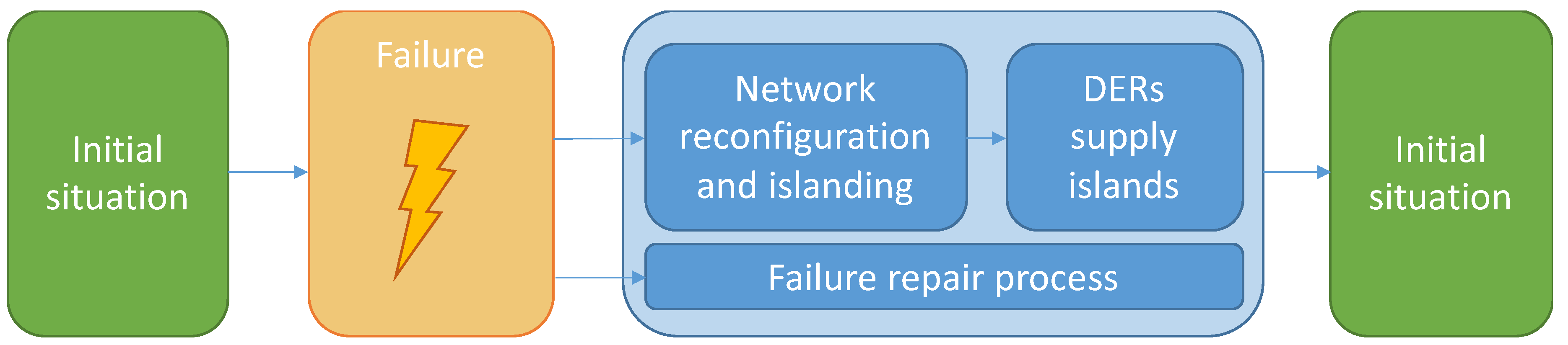
As presented in the introduction, this paper addresses the problem of improving the reliability of radial distribution networks in rural and secluded areas. Currently, when a contingency occurs in such a feeder, protection systems isolate it, and all downstream users suffer an interruption until the fault is repaired and service is restored. This paper proposes a methodology for determining the optimal size and location of a set of DERs (a combination of generators and storage), considering both reliability improvements and investment minimization. In the event of a contingency, and once the fault is isolated, the installed DERs allow to keep supplying the affected consumers while the fault is being repaired, thus minimizing the duration of the interruption times of those customers. This process is shown in Figure 1. The proposed reliability improvement application can be combined with other potential services that DERs can provide, such as voltage control or congestion management, since the islanded operation will only be used sporadically when network outages occur.
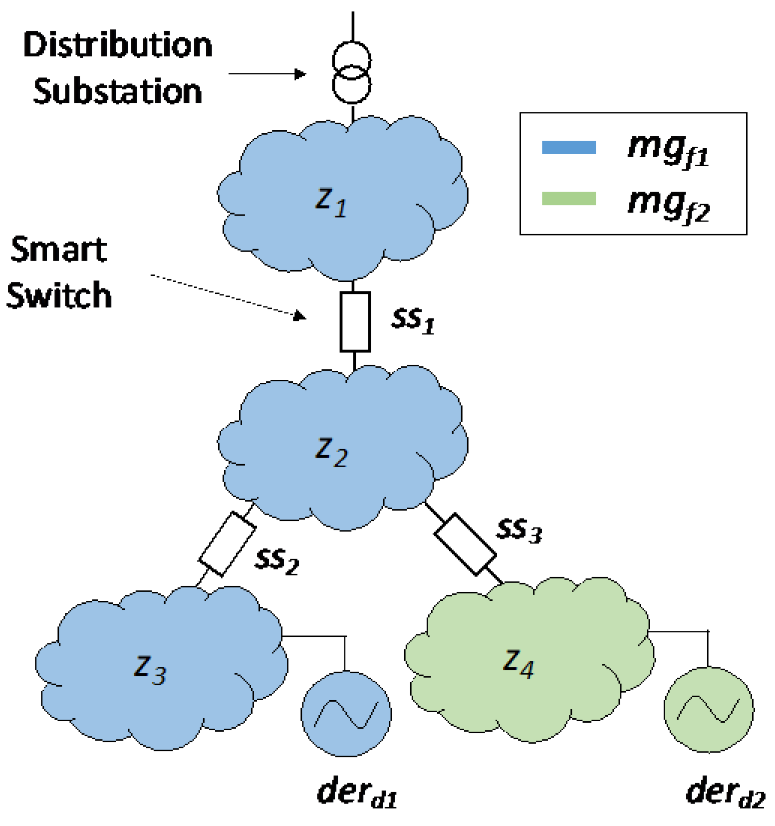
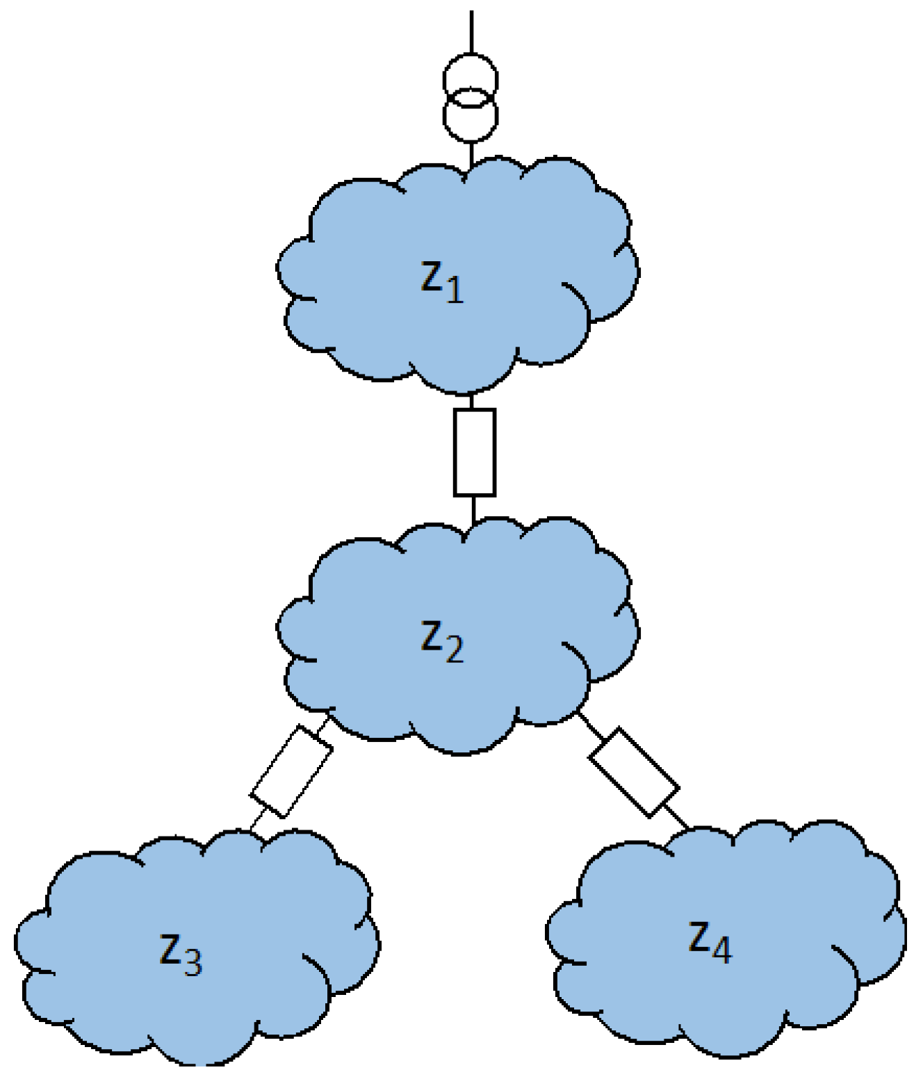
For illustrative purposes, this section provides an overview the kind of MG-based solutions that the proposed model would yield, and the main concepts used throughout the paper. However, these concepts are further detailed in Section 3. In this line, Figure 2 shows an example of a network divided into four zones (z1, z2, z3, z4). These zones are delimited by three smart switches (ss1, ss2, ss3) that enable the reconfiguration of the network when an outage occurs. This figure shows a possible solution to improve the reliability of this network. Two sets of DERs (derd1 and derd2) are installed in different zones of the system. The colors used denote that derd1 is designed to supply three zones (z1, z2, and z3), while derd2 is dimensioned to supply just z4.
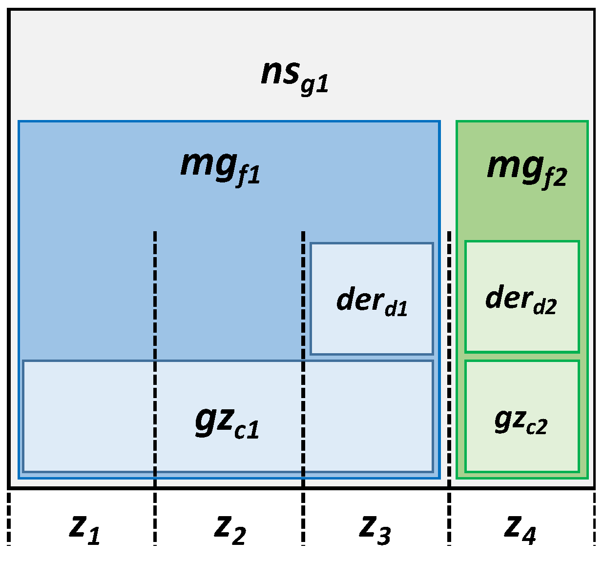
The Network Solution (nsg1) for the previous network example is described in Figure 3. The distribution network has four zones (z1, z2, z3, and z4), and two MGs (mgf1 and mgf2) designed to improve the reliability of the network. These MGs are dimensioned considering the load within two groups of zones (gzc1 and gzc2) and comprise two sets of DERs (derd1 and derd2), respectively.
Considering the same network, under a conventional scenario, when a failure takes place in z2, the nearest upstream switching element (ss1) would isolate it from the upstream grid, leaving z3 and z4 without supply, while z1 would continue being supplied from the upstream substation. However, with the Network Solution exemplified in Figure 2, the same fault in z2, would only lead to the loss of supply of the affected zone, since derd1 would supply z3, and derd2 would supply z4, while z1 would continue being supplied from the upstream substation. It should be noted that DERs would only be operated for this purpose while the failed zone is out of service, and only supplying those zones that cannot be supplied from the upstream substation due to the fault location. The rest of the time, these DERs may be used for other purposes like voltage control, energy production, or energy arbitrage in the case of batteries. It is important to note that if the contingency takes place in the same zone where the DERs are located, it is assumed that the corresponding micro-grid would lose its ability to be operated in an islanding manner. For instance, in the example of Figure 2, if the fault occurs in zone z3, the load of this zone would not be supplied, counting as non-served energy, whereas zones z1 and z2 will be supplied by the upstream substation, and derd2 would supply z4.
The methodology presented in this paper is observed from a DSO point of view. The utility can use this tool to plan the resources of its property used in case of failure, and which traditionally have consisted of diesel units. These DERs could be located in the point located further upstream of the indicated zone. In this way, the network will operate in normal conditions and congestion or voltage problems will be avoided. However, different strategies can be applied according to the wishes of the operator as described in the paper.
3. Terminology and Mathematical Formulation
The exact definitions of the concepts described in Section 2, as well as their mathematical formulation, are provided below in order to facilitate readers’ understanding of the description of the methodology in Section 4.
- Smart Switches (ssa): Tele-controlled switching devices able to isolate damaged parts of the network when a failure or contingency takes place. It is assumed that their actuation—status change to open and network reconfiguration—is fast enough to avoid worsening reliability indexes commonly counted for interruption durations longer than 3 min [27]. The set that includes all the smart switches located in the network is defined as SS, while A is the total number of elements—number of smart switches—as shown in Equation (1)
- Zone (zb): Network subset bounded by smart switches. The set that includes all the network zones is defined as Z, and B is the total number of zones. B can be obtained as the number of smart switches A plus one. The proposed notation is shown in Equation (2).
- Group of Zones (gzc): Set of adjacent network zones potentially supplied by the same generation and storage installations under islanded operation. The set that includes all the possible groups of zones is defined as GZ, and the total number is C. This value depends on the network topology and the number/location of smart switches, and it is calculated as the number of different sets of connected zones as Equation (3) shows.where:
- ○
- “P (input element)” is a function that provides the power-set of an input set, in this case, the Zones set. The power-set, in mathematics, is defined as the set of all the subsets of a set.
- ○
- “Zones (input element)” is a function that provides the set of zones of which the input element is composed.
- Distributed Energy Resources (dersd): Tuple of generation facilities and storage installations as shown in Equation (4). In this paper, different solar PV installations (pvi), diesel units (duj), and batteries (bessk) are considered. The indexes i, j, and k determines which elements of the equipment catalog are selected for each DERs design derd. The PV installations and the diesel units are defined by their rated power (kW). The storage installations are defined by their rate capacity (kWh) and their ratio power/capacity (kW/kWh). In addition, the annualized CAPEX (Capital Expenditure) and OPEX (Operating Expenditures) are considered for all the installations. The set that includes all the possible distributed energy resources combinations, according to the equipment catalog, is defined as DER, and the total number is equal to D.
Moreover, the set that includes all the optimal DERs for the group of zones gzc in terms of investment and non-served energy (reliability index) is defined as DER_OPTc as shown in Equation (5). The total number of optimal DERs for the group of zones gzc is equal to E. Thus, DER_OPTc is just the optimal subset of DER for the group of zones gzc.
- Micro-Grid (mgf): Tuple composed by a group of zones gzc, a tuple of optimal DERs der_optce feeding that group of zones, and the zone zb, where the DERs are located as shown in Equation (6).The set that includes all the possible MG designs is defined as MG, and the total number is equal to F.
- Network Solution (nsg): Subset of the micro-grids (MG) set, where all the zones are included but only once, as Equation (7) details. In other words, all the network is included in a network solution like the combination of different MGs. The set that includes all the possible network solutions is defined as NS, and the total number is equal to G.
Section 4 presents the developed methodology for obtaining the set of optimal Network Solutions to improve the continuity of supply under network contingencies while minimizing the associated investment of DER installations.
4. Methodology
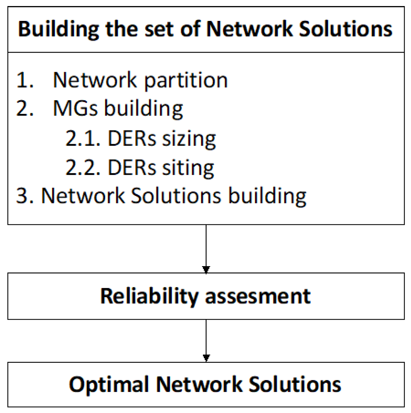
This section details the methodology developed to obtain the aforementioned Network Solutions, understood as a combination of micro-grid system designs and locations. As shown in Figure 4, the construction of the set of Network Solutions starts with a network partition based on the location of the existing smart switches. Next, based on the grid connectivity layout, all possible Groups of Zones are identified. Subsequently, the DER installations for supplying each of the Groups of Zones—and therefore the MGs—are sized and located, finding the optimal combinations of technologies for each case. This optimization is carried out attending to a double perspective: minimization of investment costs and non-supplied energy. Since this is a multicriteria optimization, the sizing step makes it possible to find several optimal DER combinations for each MG, and therefore, different Network Solutions. Finally, network reliability is assessed for each Network Solution, selecting those ones that are optimal (non-dominated solutions in the Pareto front) in terms of reliability and investment.
Broadly speaking, multicriteria optimization problems such as the one addressed herein can be tackled through two main approaches [28]. On the one hand, weights can be assigned to each of the functions to be optimized in order to obtain a single objective function which, once solved, yields a single optimal solution. This solution strongly depends on the weighting factors selected, which vary according to the planner preferences. On the other hand, a second alternative consists of evaluating all the individual objective functions separately and obtain a set of optimal, non-dominated, solutions that belong to the Pareto front. In this case, there is no longer a single solution, but a set of non-dominated ones, i.e., there is no other possible solution that performs better than these in all the separate objective functions at the same time. The methodology proposed in this paper follows this last approach.
Distribution network planning, and specifically the installation of DERs, entails important investments. Thus, it is really convenient for distribution companies to have a wide range of well-performing solutions so that they can choose the one that fits better their needs. The proposed methodology offers the advantage of obtaining all the non-dominated solutions without exploring all possible combinations. This is achieved thanks to a two-step optimization following a bottom-up approach. In the first stage, MGs are constructed sizing the DERs that minimize the MG non-served energy and investment cost. In a second step, an optimization that builds the Network Solutions with minimal non-served energy and investment is performed. Therefore, the total complexity of the whole design problem is significantly reduced. The computational burden of solving this problem is essentially determined by the number of smart switches in the feeder, as they increase the network reconfiguration possibilities. Nevertheless, the type of practical applications of the proposed planning solutions would be mostly installed in rural areas. In rural areas, the level of distribution network automation is typically low (normally between three and eight smart switches per feeder); consequently, the methodology described in this section is totally valid as demonstrated by the case study in Section 4.
In the following sub-sections, the different methodology steps, according to Figure 3, are described in depth, including the assumptions made and the developed mathematical formulation.
4.1. Network Partition
In highly automated distribution networks, as in the case addressed in this paper, when a fault occurs, a fast isolation of the faulted area and a quick network reconfiguration in MGs are essential to avoid affecting reliability indices. For this reason, the zone partition is made depending on the smart switches location. Thus, the total number of zones in which a network is divided is computed as the number of smart switches plus one. Taking as reference the example network structure represented in Figure 2 and Figure 3, the SS and Z sets are calculated, see Equations (8) and (9).
Before determining the location of DER, it is important to determine the zones they would be able to supply. For this purpose, all the possible Groups of Zones are determined. According to the definition in Equation (3), the set of all the Group of Zones GZ is determined by every group of interconnected zones that belongs to the power-set of Z. In the example, Equation (10) shows the resulting power-set of Z.
The pseudocode shown in Table 1 summarizes the process used to obtain GZ from the power-set of Z, and its total number of elements C.
Accordingly, Equation (11) presents the GZ obtained for the example network through the pseudocode in Table 1.
4.2. Micro-Grid Building
Once all the possible Groups of Zones have been obtained, the next step is MG formation. As shown in Equation (6), a MG is defined through the tuple of three elements: a Group of Zones gzc, a tuple of optimal DERs der_optce, and finally the zone za where the DER installations are located. These last two elements will be the object of study in this sub-section.
The process of obtaining the MGs is carried out in two stages. In the first one, for each Group of Zone gzc, the optimal elements of the DER set “der_optce” are determined. These are those that minimize investment costs and non-served energy. Secondly, the obtained der_optce is located in each one of all the zones za, which belongs to the considered Group of Zones gzc. This process is described as pseudocode in Table 2 however, the sizing and siting procedures will be further explained in Section 4.2.1 and Section 4.2.2 respectively.
4.2.1. DER Sizing
In this sub-section, the goal is to obtain for each one of the possible MGs, a set of optimal DERs DER_OPTc that minimizes the micro-grid non-served energy (it should be noted that the micro-grid non-served energy calculated in this section will be an upper limit, since the actual value can only be determined when the locations of the DERs and the zone where the contingency or fault occurs are established, and how each of the zones is affected by the fault (Section 4.3)) and the investment costs at the same time. Therefore, the following process is repeated for each Group of Zone gzc in order to explore all the MGs combinations.
The annualized investment (A.Inv) and operation and maintenance (O&M) cost of each DER installation are specified in an input equipment catalog (see Annex-A). Investment costs are annualized in order to compare facilities with different useful lives. The methodology used to obtain the annualized investment cost of each technology is not described since it is based on basic financial calculations and is outside the scope of the paper; however, Equation (12) aims to provide a simplified expression of the total annual DER cost calculation procedure. On the contrary, the MG non-served energy calculation associated with DER sizing and siting implies a more complex calculation and is described below.
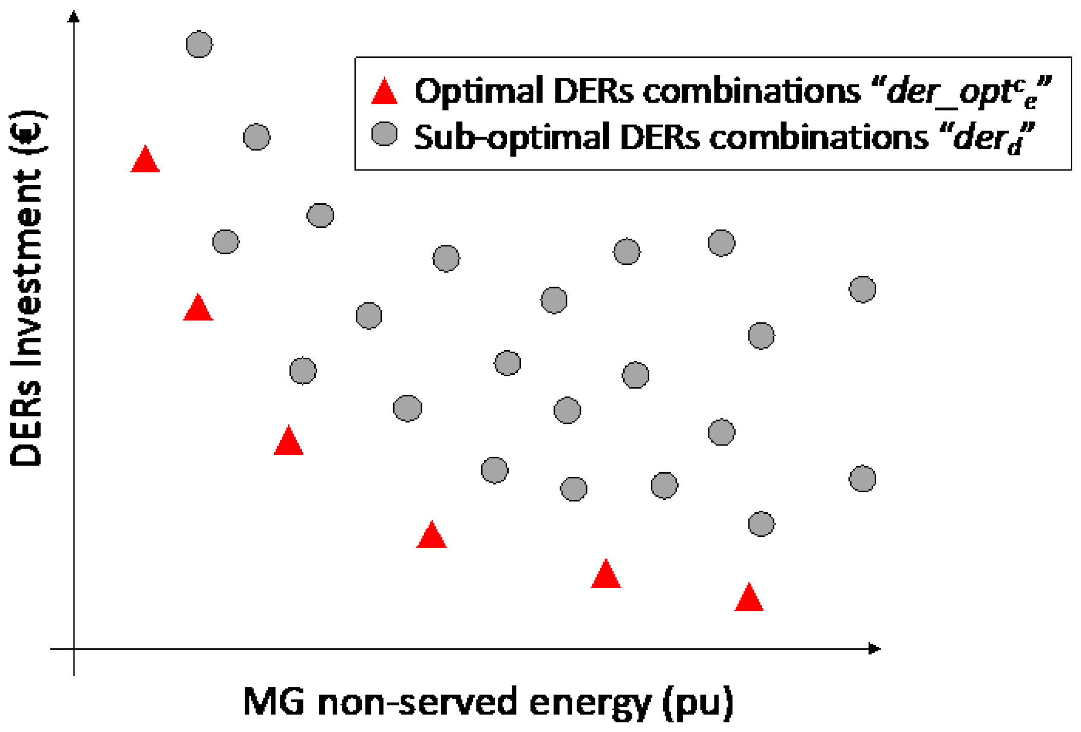
It should be noted that all selected DER technologies (solar PV, diesel units, and batteries), specified in the input catalog—DER set—are considered in each MG. Thus, those DER combinations that minimize the investment and the MG non-served energy are considered optimal and part of the DER_OPTc set, while the rest of other DER combinations are discarded. Figure 5 shows this process. The red triangles represent the optimal subset of DER for the analyzed MG—DER_OPTc—while the grey circles represent all the rest DER combinations included in the catalog—DER set.
To calculate the MGs’ non-served energy, two algorithms are used. The first one is based on the installed DER capacity (kW), while the second one is based on the energy demanded by the affected customers during the contingency. The latter is needed due to the energy-constrained operation of batteries. The capacity (kWh) and the power (kW) are the two design parameters of batteries.
NSE Computing Based on Power-Limitation
As shown in Equation (13), the micro-grid non-served energy based on the power-limitation (), during a contingency that starts at a certain hour , and with a pre-defined repair time , is calculated by adding the non-served energy during all hours () in which the failure repair is taking place.
It should be mentioned that only those hours with a generation deficit are counted according to Equation (14). In the deficit case, the difference () between the micro-grid demand () and the DER availability at that hour is computed. As previously mentioned, DERs are composed of photovoltaic generation, where () is the estimated PV production at hour h, diesel units, where () is the rated capacity (kW), and batteries, where () is the maximum power that can be delivered by the battery, as shown in Equation (15). This calculation is made for all of the hours of the year, since the demand and solar generation profiles vary hour by hour, and the hour when the fault occurs is not a priori known.
NSE Computing Based on Energy-Limitation
As previously mentioned, the existence of storage units like batteries adds inter-temporal constraints that necessarily have to be considered under an energy-based approach. Resembling the previous power-based calculation, this micro-grid non-supplied energy approach (), only accounts for those hours with a generation deficit, see Equation (16).
The difference () between the energy to be supplied to the demand () during the repair time of the fault, and the generation that can be provided by the photovoltaic panels (), the batteries () and the diesel units () is shown in Equation (17). It should be noted that the available energy storage in the battery is calculated considering the battery capacity (kWh) and the state of charge of the battery when the fault occurs ().
Combined Power and Energy-Based NSE Computing
The final micro-grid non-served energy (NSE(h)) from the hour when the fault occurs (h) and during the repair time of the fault (hrep), is calculated as the most restrictive of the two previous calculations, power-based or energy-based , according to Equation (18).
The micro-grid energy demand () during the contingency time is obtained through the sum of the hourly demands in that period according to Equation (19).
To express the micro-grid non-served energy in unitary terms, the MG non-served energy coefficient is computed as the ratio between the micro-grid non-served energy (NSE(h)) and the total demanded energy () as shown in Equation (20), assuming that the fault may equiprobably happen in any of the hours of the year.
As mentioned above, those non-dominated combinations of the DER set that minimize the non-served energy and the investment will be selected as optimal to be part of the DER_OPTc set. Only the set of optimal DER combinations will be considered in the algorithms presented in the following sections, while the rest of DER combinations will be discarded.
4.2.2. DER Siting
The location of DERs is intrinsically related to the reliability of the network. For instance, one DER combination, derd, can result in very different reliability indexes with the same investment depending on the zone where it is located as shown in the Problem Statement section. For instance, zones with a high number of customers and a reduced network length, assuming that the power lines fault rate is constant per km, would be good candidates to place a set of DERs.
Therefore, the siting algorithm simulates locating the obtained optimal DER combinations, der_optce, in all possible locations, understanding as location, each of the zones that are included in the considered Group of Zones. Thus, for each Group of Zones, gzc, and optimal set of DER, der_optce, there will be as many different micro-grids, mge, as zones are included in the corresponding Group of Zones. This algorithm is clarified in the second part of the pseudocode presented in Table 1.
4.3. Network Solution Building
After the DER siting and sizing process, the complete set of MGs is obtained. However, these MGs only include subsets of the original network; therefore, it is necessary to select different combinations of MGs that connected together form the whole distribution network. As defined in the terminology section, the set of MGs that comprises the whole network is defined as a Network Solution, nsg, and the set that includes all possible Network Solutions is defined as NS. In addition, it should be noted that all zones must be included in each of the nsg, but only once—no zone should be included in more than one MG within the same network solution. This process is carried out in two steps, as described below for our example network:
- These Groups of Zones that compose the network combinations are substituted with all the MGs that contain them to create the Network Solutions set, NS. It should be emphasized that more than one MG may contain the same group of zones.
4.4. Reliability Assesment
Once all the possible Network Solutions have been obtained, it is necessary to perform the reliability assessment of each one of them (nsg included in the NS set). In the following, the method to evaluate the reliability of the system is described. In this case, the SAIDI index is selected to measure grid reliability levels. A Zone Interaction matrix “ZInsg”, is created for each Network Solution, seeking to identify how a contingency in a given zone affects the continuity of supply in another zone. Each element of this matrix is defined by the indices b1—rows—and b2—columns—where b1 represents the analyzed zone and b2 the zone where the contingency takes place. The element value can be interpreted as the per-unit non-served energy in zb1 under a contingency in zb2. This value is equal to 0 when the zb1 is not affected by a contingency in zb2; in the case of being equal to 1, the analyzed zb1 is affected by a contingency in zb2 and cannot be supplied from any DER, thus not supplying the entire zone demand. Finally, when the zb1 is affected by a contingency in zb2, but there are DERs connected to the same MG that are able to supply totally or partially it, this element of the matrix can take a value between 0 and 1 equal to the MG non-served energy coefficient obtained in Equation (20) (see Section 4.2.1). It is important to mention that when a contingency affects one of the MG zones, but there are some zones in this MG that can still be supplied by the associated DERs, the MG non-served energy coefficient will decrease proportionally to the installed power in the non-served MG zones.
It should be noted that under normal conditions (without contingencies) the operation of the entire network is radial. Only in the contingency case is the failure zone isolated, and the rest of the zones that cannot be supplied from the upstream substation (due to the fault location) would be supplied by the DERs allocated within their associated MGs.
For illustrative purposes, the example network used in the previous sections is analyzed. This network solution is composed of two MGs, the first one “mgf1” is designed to supply z1, z2, and z3 where the derd1 are located, the second one “mgf2” is only formed by z4 where derd2 are placed. Assuming the installed power in each zone is the same, and mgf1 and mgf2 have a 0.46 pu and 0.38 pu MG non-served energy coefficients, respectively (result of Equation (20)), the obtained zone interaction matrix for the nsg1 is the one shown in Equation (21).
Once the Zone Interaction matrix ZInsg is calculated for each Network Solution, the reliability assessment for each Network Solution is carried out until complete the whole NS set. For the reliability assessment, it is necessary to consider some additional parameters, such as the number of supply points in each analyzed zone (), the average repair time of the fault in the considered zone (), and the annual failure rate of the network included in the considered zone () obtained as the sum of the product of the failure rate of overhead lines, expressed per km, times the overhead line lengths in the zone plus the product of the failure rate of underground lines, expressed per km, times the underground line lengths in the zone. Equation (22) shows the SAIDI calculation for a generic Network Solution nsg.
4.5. Optimal Non-Dominated Network Solutions
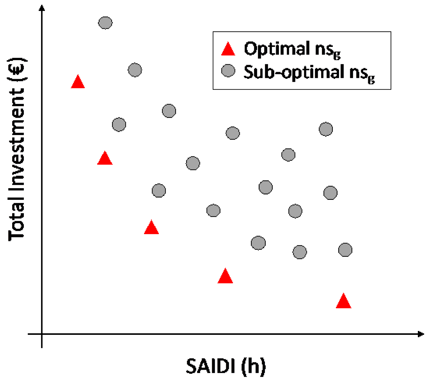
Finally, a second multi-attribute optimization is carried out in which both the calculated reliability indices and the annualized total investment costs of all the Network Solutions included in the NS set are compared. Figure 6 shows an example of the results of such optimization. In this case, the optimal—non-dominated—network solutions are represented by triangles, while sub-optimal—dominated—NS are represented by circles.
Once the Network Solutions have been selected, a specific location will be assigned for the DERs of each zone according to the established criteria, and a powerflow analysis will be carried out. Those Network Solutions that do not cause operational problems will be validated to be implemented.
5. Case Study
5.1. Description
In this section, the proposed methodology is applied to an actual distribution network. The analyzed feeder presents reliability problems. In addition, the feeder is located in a protected natural area where traditional network reinforcements are not an option due to the difficulty of obtaining permits. For this reason, the DSO in charge of supplying this area is exploring the use of non-conventional network solutions that minimize the impact on the environment.
The MV feeder analyzed presents three smart-switches and follows an identical structure as the example used for describing the proposed methodology, as shown Figure 7.
Table 4 shows the number of supply points located in each of the feeder zones, as well as the overhead and underground lengths of the power lines included in each zone.
Regarding failure rates, 12 outages/100 km-year was set for overhead lines and 6 outages/100 km-year for underground lines. Concerning the fault repair time, an average time of 6 h was considered. This data is consistent with the values posed in reference [29].
Regarding the catalog of DERs, Appendix A details the rated capacities, as well as investment and operation and maintenance costs of PV, batteries, and diesel units. It should be mentioned that the irradiation profile used to obtain PV generation is based on the geographical coordinates of the analyzed zone and obtained from [30].
5.2. Results
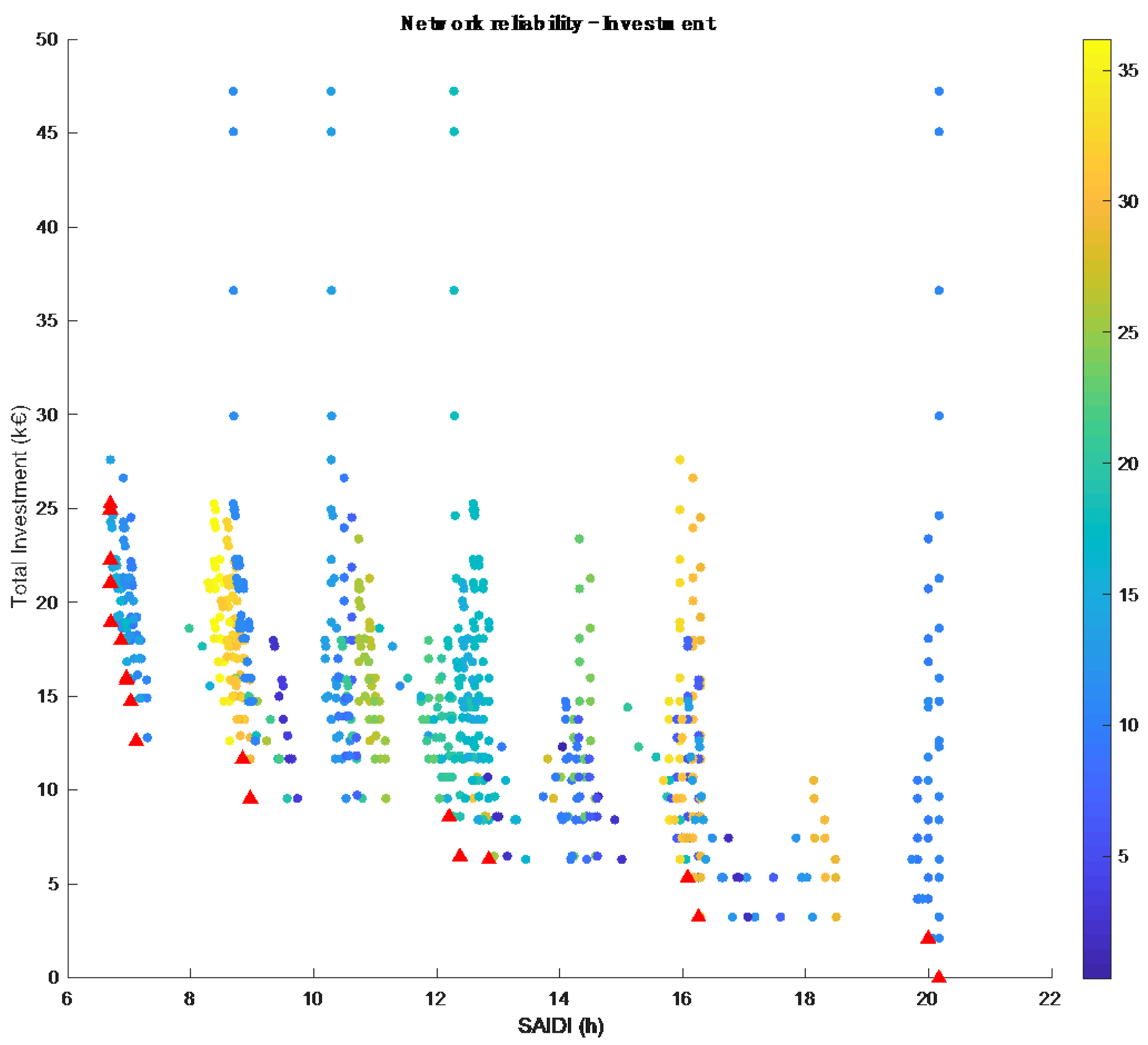
Applying the abovementioned methodology on the proposed network, 1,531 network solutions were obtained. Figure 8 shows a Pareto diagram in which the obtained reliability index (SAIDI) and the associated annualized investment in each network solution are displayed. Each of the dominated network solutions is represented by a circle, while the non-dominated solutions are represented by (red) triangles. Furthermore, in order to facilitate the selection of the solution that best suits the system needs, an additional parameter has been calculated. This parameter is, for each network solution, the standard deviation of the zonal SAIDIs with respect to the overall network SAIDI, measured in percentage. This parameter is represented by a color code in which the warmer the color the higher disparity between zonal reliability indicators. Therefore, at the same level of overall SAIDI and investment, solutions with similar reliability indices between zones (cooler colors) would be preferred ensuring more homogeneous solutions in terms of reliability.
Table 5 presents all the optimal—non-dominated—solutions ordered by their annualized investment cost, the overall SAIDI in hours, and the SAIDI standard deviation between zones. It should be noted that the Base Case (current status of the network without DERs) belongs to the set of optimal non-dominated solutions since it does not imply any investment. On the other hand, it can be seen that as the DER investment increases, solutions with better reliability (lower SAIDI) are obtained. Network solutions, such as number 10, located in the Pareto front elbow, would bring important reductions in SAIDI with moderate investment. The set of 19 optimal network solutions achieve an improvement of up to 13.5 h with an annualized investment of up to 25,263 €.
Another important issue to analyze is, for each non-dominated network solution, in which network zone DERs are located and which DER technologies are selected. Table 6 presents this information. For each network solution, it identifies in which zone the DERs are located (DERs Zone) and the zones they supply (z1, z2, z3, and z4). The size of the PV systems (PPV), batteries (PBAT and EBAT) and diesel units (PDIE) are also included. It can be seen that all the optimal solutions include DERs in zone number 3. This is an expected result since this is the area with the highest number of connected supply points and located farthest from the supply point. The same happens with zone number 4 —the zone with the second-highest number of supply points—for similar reasons.
Regarding the DER combinations selected, it is observed that all network solutions except one include diesel units, in some cases supported by batteries. These batteries have a high power (kW)–capacity (kWh) ratio, which leads to the conclusion that batteries are mainly used for peak shaving, avoiding the installation of an additional diesel unit with a low use rate. This effect can be observed by comparing the evolution of selected DERs starting from the Base Case and going through network solutions 18, 17, 16 and 15. It can be observed that as the reliability index improves, the selection of batteries (solutions 18 and 16) is alternated with that of diesel units (solutions 17 and 15). Therefore, a higher granularity in diesel unit sizes presumably would eliminate the need for batteries in the optimal network solutions.
On the other hand, it is observed that there is no optimal solution selecting PV facilities. This is mainly explained by two reasons. The first is the comparatively high PV investment cost. Nowadays, PV systems can be cost-effective when the produced energy is self-consumed and/or sold to the market during the expected life of the installation. However, in this paper, we are assuming that PV is only used to obtain benefits of its production during the small number of hours per year in which network outages take place. The second reason is that, unlike storage or diesel units, the PV production is limited to the sunlight hours. This effect is modeled through solar radiation hourly profiles for the specific network location. The use of annual profiles is recommended to capture seasonality. For example, if the network failure occurs at night or at the end of the day, PV will not be able to provide the necessary energy to supply the isolated customers and to improve the continuity of supply indices.
Therefore, it can be concluded that for the network studied, and with current investment costs, the use of diesel units by themselves or in combination with batteries is the most cost-effective network solution to increase the reliability of the system. During network faults, the diesel units would cover the base demand and the batteries would cover the peaks of the isolated supply points.
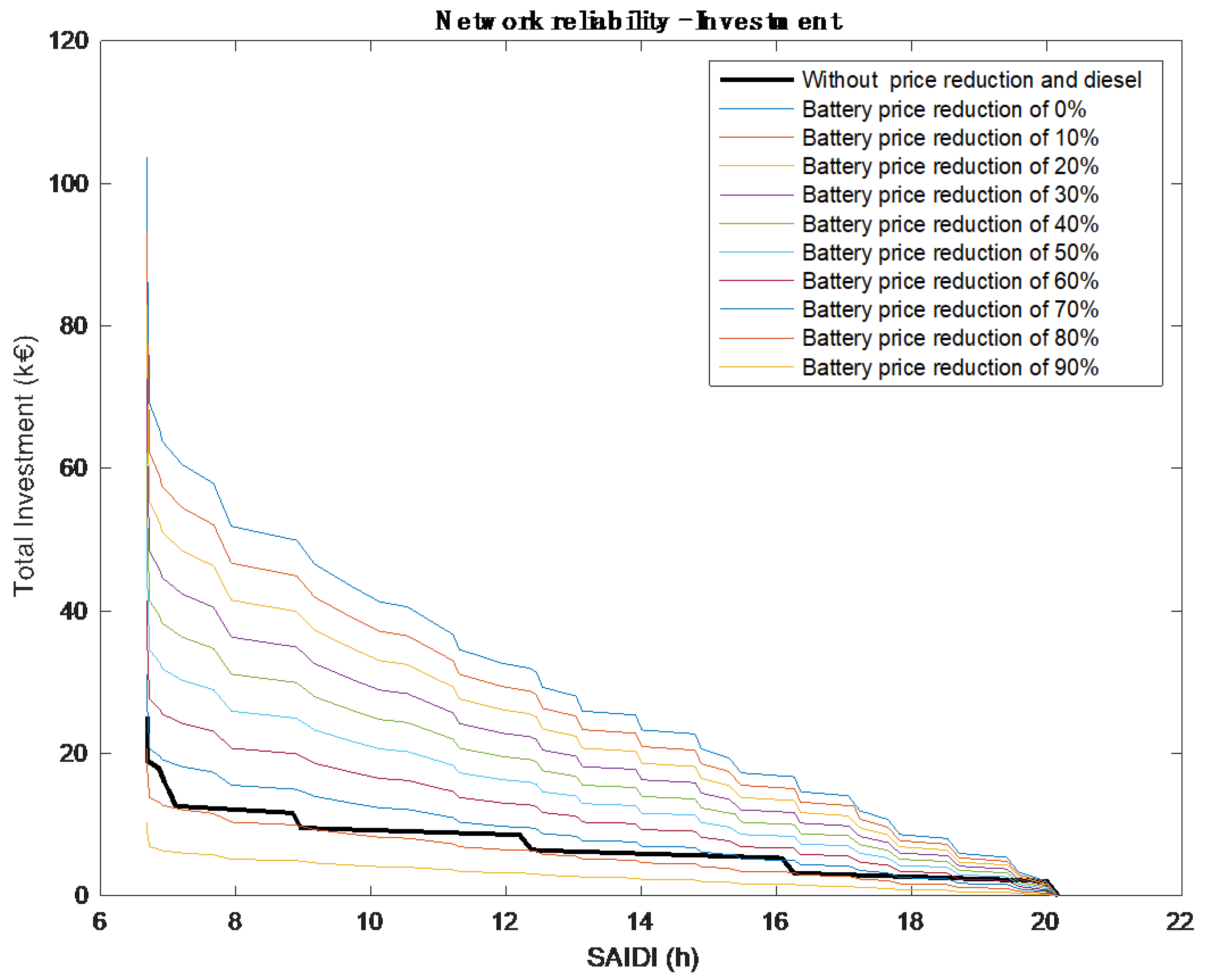
A sensitivity analysis to the investment cost of the batteries was performed. To isolate the effect of this parameter, a new case was run for which battery systems were the only DER technology available. There are four reasons for this. Firstly, batteries are less environmentally pollutant than diesel units (at least locally). Additionally, batteries are already being used in the optimal solutions of 6. Secondly, PV systems do not seem to be a good option to improve system reliability because their use is restricted to the sunlight hours and, therefore, they cannot be used when outages occur at night. Moreover, unlike batteries, in none of the 18 optimal network solutions the PV systems are chosen as a design option, being more cost-effective to invest in batteries. Third, diesel units are a mature technology from which no major price variations are expected. In this case, the only factor that could increase their cost would be a sharp rise in the cost of diesel (variable cost included in the O&M cost defined in the Annex). However, these are units that operate very few hours per year and are therefore not very sensitive to this factor. Finally, the cost of batteries nowadays presents a steady downwards trend. Therefore, the break-even point for batteries to become the preferred design option was evaluated.
Figure 9 shows the Pareto front for different percentages of battery cost reductions. It can be observed that to obtain a Pareto front similar to the one presented with current investment prices for PV and batteries and including diesel units, reductions in the cost of batteries by close to 80% would be needed.
Analyzing the results obtained, it can be concluded that diesel generators and batteries (as long as their initial state of charge is sufficient) are the preferred option, since, unlike PV systems, they are available at any time of the day and under any atmospheric conditions. This does not mean that PV systems cannot be used for this purpose, but they do have some features that make them difficult to apply. However, each case must be studied individually and new clean and hybrid solutions such as PV systems with batteries should be considered in future low-cost scenarios.
6. Conclusions
This paper proposes a novel methodology for determining the optimal location and sizing of MGs based on a multicriteria optimization in which both the DER investment cost and the network reliability levels are considered. Unlike other publications, this methodology allows the mix of DERs to be selected that best fits the needs of the network. Additionally, the result is a set of non-dominated solutions, allowing the DSO to select the one that best suits other possible non-modeled requirements (e.g., local emissions). This methodology was tested in a real case study, from which some relevant findings have been extracted, as discussed below.
The results show that the combination of diesel units and batteries seems to be the most cost-effective option to increase the reliability of the network through islanded operation. During the failure repair time, diesel units would be in charge of covering the base demand of islanded zones, whereas batteries would operate as peaking units. Moreover, the results show that selecting solar PV installations for this purpose is not cost-effective. The reason for this is twofold. On the one hand, PV presents a comparatively high investment cost. On the other hand, PV can only supply the demand during sunlight hours, thus being useless to tackle outages occurring at night. However, each case must be studied individually and adjusted to the specific climatic conditions of the network location. Finally, it has been shown that if battery investment costs were to drop by close to 80% with respect to current values, MG solutions based mainly on batteries instead of more highly polluting solutions based on diesel units would be the preferred option.
As observed in the case study, emission-free DERs are expensive and are only used in less than 1% of the hours to enhance the reliability of the distribution grid. For this reason, DSOs may explore the procurement of a service through which third parties, such as DER owners, would provide network support when a network outage takes place. The remuneration of this service would be based on the location of the DER in the network and its commitment to offering the service when requested. In this way, the DSO would reduce investments in network infrastructure and the owners of DERs could obtain additional benefits to the regular ones derived from their participation in the market or cost-savings thanks to behind the meter generation.
This work opens up future research lines to be explored. The main limitation of this study is the degree of automation of the network. The greater the degree of automation of the network, the greater the number of smart-switches, and the possibilities of reconfiguring the network would grow exponentially. For this reason, the proposed solution perfectly fits with the problems of rural networks, which are characterized by low automation levels. However, urban areas with higher automation levels may sharply increase the computational load. For this reason, this limitation opens, for example, a future research line in applying metaheuristic algorithms (e.g., genetics algorithms) to overcome this issue.
Author Contributions
Conceptualization, F.P.M., C.M.D., T.G.S.R. and R.C.A.; methodology, F.P.M., C.M.D. and T.G.S.R.; software, F.P.M. and C.M.D.; validation, F.P.M., C.M.D., T.G.S.R. and R.C.A.; writing—review and editing, F.P.M., C.M.D., T.G.S.R. and R.C.A. All authors have read and agreed to the published version of the manuscript.
Funding
This research has received funding from the Fundación Iberdrola España through the ‘Ayudas a la investigación 2019′ program.
Acknowledgments
The authors would like to thank i-DE for partially supporting this research. In particular, comments and suggestions for improving the practical application of the developed algorithms are acknowledged to Diego Haro Ginés, Roberto García Gómez, Fernando Palacios González, and Cristina Vilá Castro.
Conflicts of Interest
The authors declare no conflict of interest.
Appendix A. DER Investment
The investment in DERs is based on a review of the state of the art of the technologies employed: PV systems, battery-based storage, and diesel units.
The price of the PV systems is composed of the cost of the panels, the cost of the inverter, and the cost of installation. The cost of the panels is based on [31]. For the rest of the costs like de O&M cost, a breakdown according to the reference has been considered. The useful life is based on [32]. Table A1. shows the data used.

Table A1.
PV systems data.
| Rated Capacity (kW) | Investment Cost (€/kW) |
|---|---|
| 0 | 850 |
| 100 | O&M (€/kW-year) |
| 200 | 18.08 |
| 400 | Useful life (years) |
| 800 | 23 |
The price of the batteries is based on [33]. Other additional costs like de O&M costs have been considered according to the breakdown given in [34]. For the power-capacity ratio, the costs indicated in [32] have been taken into account. To obtain the total investment cost of batteries for different power-capacity ratios, the power and energy values are averaged. The useful life considers that very few charge/discharge cycles are expected per year in this application. Table A2 shows the data used.
Table A2.
Batteries data.
| Rated Power (kW) | Power (kW)—Capacity (kWh) Ratio | Investment Cost (€/kW) |
|---|---|---|
| 0 | 3.33 | 314.26 |
| 100 | 1 | Investment cost (€/kWh) |
| 200 | 0.4 | 346.21 |
| 400 | 0.25 | O&M (€/kWh) |
| 800 | 0.356 | |
| Useful life (years) | ||
| 15 |
The price of diesel units depends mainly on their rated capacity [35]. Apart from the price of the diesel unit itself, an installation cost of 60% was considered. For the fuel, a cost of 1.3 €/L and an expense of 0.3l/kWh has been assumed [36] to obtain the total O&M cost. A useful life of 20 years is considered, assuming that the unit will be used only a few hours per year. Table A3 shows the data used.
Table A3.
Diesel units data.
| Rated Capacity (kW) | Investment Cost (€/kW) | O&M (€/kW-year) |
|---|---|---|
| 0 | 0 | 8 |
| 100 | 223.34 | O&M (€/kWh) |
| 200 | 125.76 | 0.3 |
| 400 | 121.26 | Useful life (years) |
| 20 |
References
- European Commission. Digitalisation of the Energy Sector; SETIS Magazine; European Commission: Brussels, Belgium, 2018. [Google Scholar]
- Makris, P.; Efthymiopoulos, N.; Nikolopoulos, V.; Pomazanskyi, A.; Irmscher, B.; Stefanov, K.; Pancheva, K.; Varvarigos, E. Digitization Era for Electric Utilities: A Novel Business Model Through an Inter-Disciplinary S/W Platform and Open Research Challenges. IEEE Access 2018, 6, 22452–22463. [Google Scholar] [CrossRef]
- Staschus, K. ENTSO-E Memo 2011; Secretariat of ENTSO-E: Brussels, Belgium, 2011. [Google Scholar]
- Pavla Mandatova; Gunnar Lorenz. Power Distribution in Europe: Facts & Figures; Eurelectric: Brussels, Belgium, 2013. [Google Scholar]
- Short, T.A. Electric Power Distribution Handbook; CRC Press: Boca Raton, FL, USA, 2014. [Google Scholar]
- Electric Power Distribution Engineering. Available online: https://www.crcpress.com/Electric-Power-Distribution-Engineering-Third-Edition/Gonen/p/book/9781482207002 (accessed on 20 February 2019).
- Pérez-Arriaga, I.J. Regulation of the Power Sector; Springer: New York, NY, USA, 2013; ISBN 978-1-4471-5033-6. [Google Scholar]
- Chen, T.-H.; Huang, W.-T.; Gu, J.-C.; Pu, G.C.; Hsu, Y.F.; Guo, T.Y. Feasibility study of upgrading primary feeders from radial and open-loop to normally closed-loop arrangement. IEEE Trans. Power Syst. 2004, 19, 1308–1316. [Google Scholar] [CrossRef] [Green Version]
- Lasseter, R.H.; Paigi, P. Microgrid: A conceptual solution. In Proceedings of the 2004 IEEE 35th Annual Power Electronics Specialists Conference (IEEE Cat. No.04CH37551), Aachen, Germany, 20–25 June 2004; Volume 6, pp. 4285–4290. [Google Scholar]
- Hatziargyriou, N.; Asano, H.; Iravani, R.; Marnay, C. Microgrids. IEEE Power Energy Mag. 2007, 5, 78–94. [Google Scholar] [CrossRef]
- Marnay, C.; Asano, H.; Papathanassiou, S.; Strbac, G. Policymaking for microgrids. IEEE Power Energy Mag. 2008, 6, 66–77. [Google Scholar] [CrossRef]
- Pérez-Arriaga, J.I.; Batlle, C.; Gómez, T.; Chaves, J.P.; Rodilla, P.; Herrero, I.; Dueñas, P.; Ramírez, C.R.V.; Bharatkumar, A.; Burger, S.; et al. Utility of the Future: An MIT Energy Initiative Response to an Industry in Transition; Massachusetts Institute of Technology: Cambridge, MA, USA, 2016. [Google Scholar]
- Types of Microgrids|Building Microgrid. Available online: https://building-microgrid.lbl.gov/types-microgrids (accessed on 10 April 2020).
- Asmus, P.; Lawrence, M. Emerging Microgrid Business Models. Available online: /paper/Emerging-Microgrid-Business-Models-Asmus-Lawrence/67052852b5b104d9e7f61daaa1b7220d74cdb39d (accessed on 9 June 2020).
- Rocabert, J.; Luna, A.; Blaabjerg, F.; Rodríguez, P. Control of Power Converters in AC Microgrids. IEEE Trans. Power Electron. 2012, 27, 4734–4749. [Google Scholar] [CrossRef]
- Lopes, J.A.P.; Moreira, C.L.; Madureira, A.G. Defining control strategies for MicroGrids islanded operation. IEEE Trans. Power Syst. 2006, 21, 916–924. [Google Scholar] [CrossRef] [Green Version]
- Lasseter, R.H. Smart Distribution: Coupled Microgrids. Proc. IEEE 2011, 99, 1074–1082. [Google Scholar] [CrossRef]
- Patel, Y.P.; Patel, A.G. Placement of DG in Distribution System for loss reduction. In Proceedings of the 2012 IEEE Fifth Power India Conference, Delhi, India, 19–22 December 2012; pp. 1–6. [Google Scholar]
- Anand, S.; Fernandes, B.G.; Guerrero, J. Distributed Control to Ensure Proportional Load Sharing and Improve Voltage Regulation in Low-Voltage DC Microgrids. IEEE Trans. Power Electron. 2013, 28, 1900–1913. [Google Scholar] [CrossRef] [Green Version]
- Armendáriz, M.; Heleno, M.; Cardoso, G.; Mashayekh, S.; Stadler, M.; Nordström, L. Coordinated microgrid investment and planning process considering the system operator. Appl. Energy 2017, 200, 132–140. [Google Scholar] [CrossRef] [Green Version]
- Ciller, P.; Ellman, D.; Vergara, C.; González-García, A.; Lee, S.J.; Drouin, C.; Brusnahan, M.; Borofsky, Y.; Mateo, C.; Amatya, R.; et al. Optimal Electrification Planning Incorporating On- and Off-Grid Technologies: The Reference Electrification Model (REM). Proc. IEEE 2019, 107, 1872–1905. [Google Scholar] [CrossRef]
- Park, W.Y.; Shah, N.; Phadke, A. Enabling access to household refrigeration services through cost reductions from energy efficiency improvements. Energy Effic. 2019, 12, 1795–1819. [Google Scholar] [CrossRef] [Green Version]
- DeForest, N.; MacDonald, J.S.; Black, D.R. Day ahead optimization of an electric vehicle fleet providing ancillary services in the Los Angeles Air Force Base vehicle-to-grid demonstration. Appl. Energy 2018, 210, 987–1001. [Google Scholar] [CrossRef] [Green Version]
- Celli, G.; Ghiani, E.; Mocci, S.; Pilo, F. A multi-objective formulation for the optimal sizing and siting of embedded generation in distribution networks. In Proceedings of the 2003 IEEE Bologna Power Tech Conference Proceedings, Bologna, Italy, 23–26 June 2003; Volume 1, p. 8. [Google Scholar]
- Ippolito, M.G.; Morana, G.; Sanseverino, E.R.; Vuinovich, F. Risk based optimization for strategical planning of electrical distribution systems with dispersed generation. In Proceedings of the 2003 IEEE Bologna Power Tech Conference Proceedings, Bologna, Italy, 23–26 June 2003; Volume 1, p. 7. [Google Scholar]
- Popović, D.H.; Greatbanks, J.A.; Begović, M.; Pregelj, A. Placement of distributed generators and reclosers for distribution network security and reliability. Int. J. Electr. Power Energy Syst. 2005, 27, 398–408. [Google Scholar] [CrossRef]
- Tabatabaei, N.M.; Ravadanegh, S.N.; Bizon, N. (Eds.) Power Systems Resilience: Modeling, Analysis and Practice; Springer International Publishing: Cham, Switzerland, 2019; ISBN 978-3-319-94441-8. [Google Scholar]
- Ehrgott, M. Multicriteria Optimization, 2nd ed.; Springer-Verlag: Berlin/Heidelberg, Germany, 2005; ISBN 978-3-540-21398-7. [Google Scholar]
- Kjolle, G.; Sand, K. RELRAD-an analytical approach for distribution system reliability assessment. IEEE Trans. Power Deliv. 1992, 7, 809–814. [Google Scholar] [CrossRef]
- Renewables.ninja. Available online: https://www.renewables.ninja/ (accessed on 7 April 2020).
- Magazine, pv Module Price Index. Available online: https://www.pv-magazine.com/features/investors/module-price-index/ (accessed on 10 April 2020).
- McLaren, J.; Gagnon, P.; Anderson, K.; Elgqvist, E.; Fu, R.; Remo, T. Battery Energy Storage Market: Commercial Scale, Lithium-ion Projects in the U.S.; National Renewable Energy Lab. (NREL): Golden, CO, USA, 2016. [Google Scholar]
- Worldwide - lithium ion battery pack costs 2019. Available online: https://www.statista.com/statistics/883118/global-lithium-ion-battery-pack-costs/ (accessed on 9 April 2020).
- Wilson, M. Lazard’s Levelized Cost of Storage Analysis—Version 4.0; Lazard: New Orleans, LA, USA, 2018. [Google Scholar]
- What is the average price of the generator sets? Available online: https://grupoelectrogeno.net/precio-medio-grupos-electrogenos/ (accessed on 9 April 2020).
- Precio en España de Ud de Grupo electrógeno. Generador de precios de la construcción. CYPE Ingenieros, S.A. Available online: http://www.generadordeprecios.info/obra_nueva/Instalaciones/Electricas/Generadores_de_energia_electrica/Grupo_electrogeno.html (accessed on 9 April 2020).
Figure 1.
Action plan when a contingency occurs.

Figure 2.
Example of a selected Network Solution.

Figure 3.
Nomenclature diagram for a selected Network Solution.

Figure 4.
Methodology flowchart.

Figure 5.
Pareto optimization for DER combinations for each analyzed MG.

Figure 6.
Pareto optimization for NS.

Figure 7.
Network structure.

Figure 8.
Network solutions for the case study network (colors represent the standard deviation of zonal SAIDI in percentage).
Figure 8.
Network solutions for the case study network (colors represent the standard deviation of zonal SAIDI in percentage).

Figure 9.
Pareto fronts for different battery price reductions.

Table 1.
Pseudocode for the Group of Zones GZ formation.
| Pseudocode |
|---|
| GZ = ø; c = 0 |
| for each “element” in P(Z) |
| if the “element” is connected |
| Add “element” to GZ |
| c += 1 |
Table 2.
Pseudocode for the Micro-Grids MG formation.
| Pseudocode |
|---|
 |
Table 3.
Network combinations for the example network.
| Combination Number | Network Combination |
|---|---|
| 1 | |
| 2 | |
| 3 | |
| 4 | |
| 5 | |
| 6 | |
| 7 |
Table 4.
Network characteristics.
| Zone | Number of Supply Points | Overhead Length (km) | Underground Length (km) |
|---|---|---|---|
| z1 | 0 | 10.99 | 0.04 |
| z2 | 585 | 9.54 | 0.82 |
| z3 | 1386 | 9.94 | 2.07 |
| z4 | 771 | 6.04 | 0.15 |
Table 5.
Optimal network solutions for the case study network.
| nsg | Annualized Investment (€) | SAIDI Overall Network (h) | SAIDI Reduction (%) | SAIDI Standard Deviation (%) | SAIDIz1 (h) | SAIDIz2 (h) | SAIDIz3 (h) | SAIDIz4 (h) |
|---|---|---|---|---|---|---|---|---|
| 1 | 25,263 | 6.7 | −67% | 14% | 7.8 | 7.1 | 4.4 | 0.0 |
| 2 | 24,945 | 6.7 | −67% | 14% | 7.8 | 7.1 | 4.4 | 0.0 |
| 3 | 22,291 | 6.7 | −67% | 14% | 7.8 | 7.1 | 4.4 | 0.0 |
| 4 | 21,052 | 6.7 | −67% | 14% | 7.8 | 7.1 | 4.4 | 0.0 |
| 5 | 18,947 | 6.7 | −67% | 14% | 7.8 | 7.1 | 4.4 | 0.0 |
| 6 | 17,980 | 6.9 | −66% | 16% | 8.1 | 7.2 | 4.4 | 0.0 |
| 7 | 15,975 | 6.9 | −66% | 13% | 8.0 | 7.3 | 4.8 | 0.0 |
| 8 | 15,875 | 7 | −65% | 17% | 8.3 | 7.2 | 4.4 | 0.0 |
| 9 | 14,736 | 7 | −65% | 14% | 8.1 | 7.3 | 4.8 | 0.0 |
| 10 | 12,632 | 7.1 | −65% | 15% | 8.3 | 7.3 | 4.8 | 0.0 |
| 11 | 11,664 | 8.8 | −56% | 32% | 8.3 | 15.0 | 5.1 | 0.0 |
| 12 | 9560 | 9 | −55% | 30% | 8.3 | 15.0 | 5.6 | 0.0 |
| 13 | 8592 | 12.2 | −40% | 19% | 14.7 | 15.0 | 5.6 | 0.0 |
| 14 | 6488 | 12.4 | −39% | 19% | 15.1 | 15.0 | 5.6 | 0.0 |
| 15 | 6316 | 12.8 | −37% | 17% | 8.3 | 15.0 | 19.4 | 0.0 |
| 16 | 5348 | 16.1 | −20% | 7% | 14.7 | 15.0 | 19.4 | 0.0 |
| 17 | 3244 | 16.3 | −19% | 7% | 15.1 | 15.0 | 19.4 | 0.0 |
| 18 | 2105 | 20 | −1% | 11% | 22.4 | 15.0 | 19.4 | 0.0 |
| Base Case | 0 | 20.2 | 0% | 11% | 22.8 | 15.0 | 19.4 | 0.0 |
Table 6.
Optimal network solutions for the case study network.
| nsg | DERs Zone | z1 | z2 | z3 | z4 | PPV (kW) | PBAT (kW) | EBAT (kWh) | PDIE (kW) |
|---|---|---|---|---|---|---|---|---|---|
| 1 | 2 | 0 | 1 | 0 | 0 | 0 | 0 | 0 | 200 |
| 3 | 0 | 0 | 1 | 0 | 0 | 0 | 0 | 400 | |
| 4 | 0 | 0 | 0 | 1 | 0 | 0 | 0 | 200 | |
| 2 | 3 | 0 | 1 | 1 | 0 | 0 | 100 | 250 | 400 |
| 4 | 0 | 0 | 0 | 1 | 0 | 0 | 0 | 200 | |
| 3 | 3 | 0 | 1 | 1 | 0 | 0 | 100 | 100 | 400 |
| 4 | 0 | 0 | 0 | 1 | 0 | 0 | 0 | 200 | |
| 4 | 3 | 0 | 1 | 1 | 0 | 0 | 100 | 30 | 400 |
| 4 | 0 | 0 | 0 | 1 | 0 | 0 | 0 | 200 | |
| 5 | 3 | 0 | 1 | 1 | 0 | 0 | 0 | 0 | 400 |
| 4 | 0 | 0 | 0 | 1 | 0 | 0 | 0 | 200 | |
| 6 | 2 | 0 | 1 | 0 | 0 | 0 | 0 | 0 | 100 |
| 3 | 0 | 0 | 1 | 0 | 0 | 100 | 30 | 200 | |
| 4 | 0 | 0 | 0 | 1 | 0 | 0 | 0 | 200 | |
| 7 | 3 | 0 | 0 | 1 | 0 | 0 | 100 | 100 | 200 |
| 4 | 0 | 1 | 0 | 1 | 0 | 0 | 0 | 200 | |
| 8 | 2 | 0 | 1 | 0 | 0 | 0 | 0 | 0 | 100 |
| 3 | 0 | 0 | 1 | 0 | 0 | 0 | 0 | 200 | |
| 4 | 0 | 0 | 0 | 1 | 0 | 0 | 0 | 200 | |
| 9 | 3 | 0 | 0 | 1 | 0 | 0 | 100 | 30 | 200 |
| 4 | 0 | 1 | 0 | 1 | 0 | 0 | 0 | 200 | |
| 10 | 3 | 0 | 0 | 1 | 0 | 0 | 0 | 0 | 200 |
| 4 | 0 | 1 | 0 | 1 | 0 | 0 | 0 | 200 | |
| 11 | 3 | 0 | 0 | 1 | 0 | 0 | 0 | 0 | 200 |
| 4 | 0 | 0 | 0 | 1 | 0 | 100 | 30 | 100 | |
| 12 | 3 | 0 | 0 | 1 | 0 | 0 | 0 | 0 | 200 |
| 4 | 0 | 0 | 0 | 1 | 0 | 0 | 0 | 100 | |
| 13 | 3 | 0 | 0 | 1 | 0 | 0 | 100 | 30 | 100 |
| 4 | 0 | 0 | 0 | 1 | 0 | 0 | 0 | 100 | |
| 14 | 3 | 0 | 0 | 1 | 0 | 0 | 0 | 0 | 100 |
| 4 | 0 | 0 | 0 | 1 | 0 | 0 | 0 | 100 | |
| 15 | 3 | 0 | 0 | 1 | 0 | 0 | 0 | 0 | 200 |
| 16 | 3 | 0 | 0 | 1 | 0 | 0 | 100 | 30 | 100 |
| 17 | 3 | 0 | 0 | 1 | 0 | 0 | 0 | 0 | 100 |
| 18 | 3 | 0 | 0 | 1 | 0 | 0 | 100 | 30 | 0 |
© 2020 by the authors. Licensee MDPI, Basel, Switzerland. This article is an open access article distributed under the terms and conditions of the Creative Commons Attribution (CC BY) license (http://creativecommons.org/licenses/by/4.0/).
Share and Cite
MDPI and ACS Style
Postigo Marcos, F.; Mateo Domingo, C.; Gómez San Román, T.; Cossent Arín, R. Location and Sizing of Micro-Grids to Improve Continuity of Supply in Radial Distribution Networks. Energies 2020, 13, 3495. https://doi.org/10.3390/en13133495
AMA Style
Postigo Marcos F, Mateo Domingo C, Gómez San Román T, Cossent Arín R. Location and Sizing of Micro-Grids to Improve Continuity of Supply in Radial Distribution Networks. Energies. 2020; 13(13):3495. https://doi.org/10.3390/en13133495
Chicago/Turabian StylePostigo Marcos, Fernando, Carlos Mateo Domingo, Tomás Gómez San Román, and Rafael Cossent Arín. 2020. "Location and Sizing of Micro-Grids to Improve Continuity of Supply in Radial Distribution Networks" Energies 13, no. 13: 3495. https://doi.org/10.3390/en13133495
Note that from the first issue of 2016, this journal uses article numbers instead of page numbers. See further details here.