Series DC Arc Simulation of Photovoltaic System Based on Habedank Model

1
Department of Illuminating Engineering and Light Sources, School of Information Science and Technology, Fudan University, Shanghai 200433, China
2
Shanghai Engineering Research Center for Artificial Intelligence Integrated Energy System, Fudan University, Shanghai 200433, China
3
Innovation Institute of ISoftStone, ISoftStone Co., Ltd., Beijing 100193, China
*
Author to whom correspondence should be addressed.
Energies 2020, 13(6), 1416; https://doi.org/10.3390/en13061416
Submission received: 14 February 2020
/
Revised: 12 March 2020
/
Accepted: 13 March 2020
/
Published: 18 March 2020
(This article belongs to the Section A2: Solar Energy and Photovoltaic Systems)
Abstract
:Despite the rapid development of photovoltaic (PV) industry, direct current (DC) fault arc remains a major threat to the safety of PV system and personnel. While extensive research on DC fault arc has been conducted, little attention has been paid to the long-time interactions between the PV system and DC arc. In this paper, a simulation system with an arc model and PV system model is built to overcome the inconvenience of the fault-arc experiments and understand the mechanism of these interactions. For this purpose, the characteristics of the series DC arc in a small grid-connected PV system are first investigated under uniform irradiance. Then, by comparing with different arc models, the Habedank model is selected to simulate the fault arc and a method to determine its parameters under DC arc condition is proposed. The trends of simulated arc waveforms are consistent with the measured data, whose fitting degree in adjusted R-squared is between 0.946 and 0.956. Finally, a phenomenon observed during the experiment, that the negative perturbation of the maximum power point tracking (MPPT) algorithm can reduce the arc current, is explained by the proposed model.
1. Introduction
The direct current (DC) fault arc is essentially a gas discharging phenomenon. The huge amount of heat released by the burning arc can easily ignite the surrounding combustible materials [1], which leads to fire hazard and malfunction of the photovoltaic (PV) system. The earliest recorded fire hazard at a PV station caused by DC fault arc dates back to the 1990s [2]. With the rapid growth of PV installed capacity, DC fault arc becomes a potential danger that cannot be ignored. In 2011, an arc-fault interrupter was firstly required in PV systems above 80 V by the National Electrical Code (NEC) [3]. In the same year, the Underwriter Laboratories published UL 1699b, which specifies the test standards of arc-fault circuit interrupters; for example, the arcing time before the operation of interrupter should not exceed 2 s [4]. Since then, the DC fault arc in PV systems has attracted extensive attention from academia and industry.
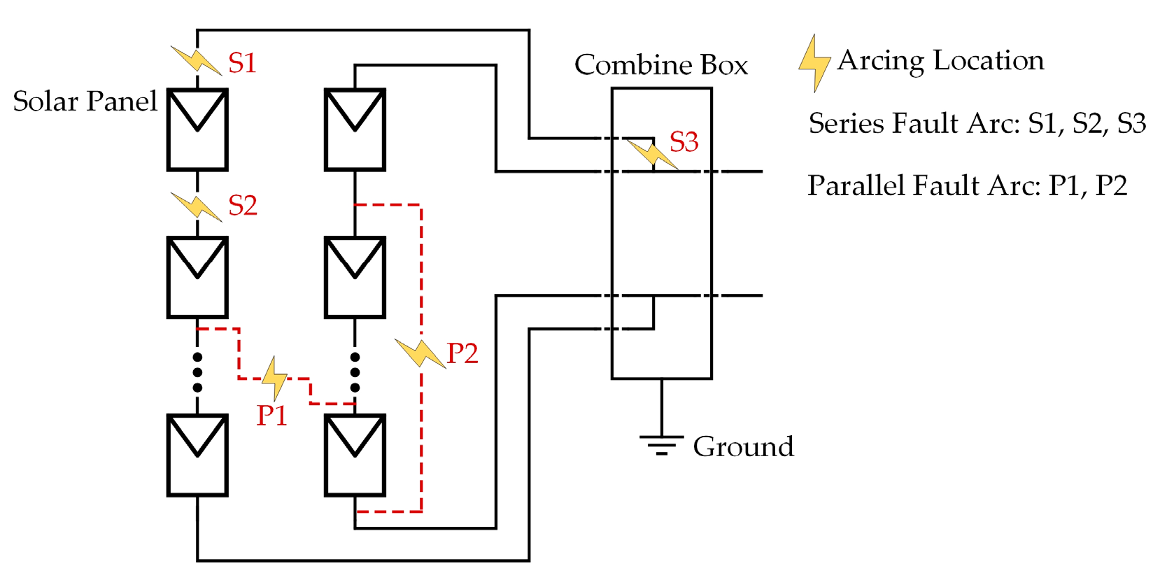
The DC fault arcs in PV systems can be classified into series and parallel arcs (Figure 1). A series arc is usually formed by disconnection of a conductive circuit, while a parallel arc is caused by the failure of conductor insulation. The series arc can be extinguished by disconnecting the strings, and, in order to extinguish parallel arc, the strings affected by parallel arc should be shorted. In the past few years, the focus of academic research has been on detecting DC fault arcs in PV systems. The burning arc can generate sound, light, and electromagnetic wave which can be used as criteria to detect the arc [5,6]. On the other hand, when an arc is generated, it becomes a part of the PV system, which means it can affect the circuit signals of the PV system. The current and voltage signals of PV systems are used by most researchers to extract the arc characteristic signals. An important discovery that the arcing noise mainly exists in the 10–100 kHz frequency band was made by Sandia National Laboratories (SNL) [7]. In addition, because the methods used to extinguish series and parallel arcs are different, three ways to differentiate series and parallel arcs were proposed in [8]. Until now, many different DC arc detection methods have been proposed, including time-frequency domain detection [9,10,11,12,13,14], artificial intelligence [15,16,17,18,19], spread spectrum time domain reflectometry (SSTDR) [20], arc current entropy [21], and blind-source separation [22].
Arc-fault detection mainly focuses on the changes of PV systems within 2 s after arc ignition according to the suggestion of UL 1699b, while the long-time response of PV systems addresses less attention of researchers. In fact, in order to have a profound understanding of the interactions between arc and PV system, both short- and long-time arc-caused reaction of PV systems should be well studied. Because of the inconvenience of arc-fault experiment and the difficulty of achieving specific experimental conditions such as temperature and irradiance, the influence of arc on the PV system under different conditions can be effectively analyzed through simulation. With the help of modern computer technology, the use of complex arc models has become possible. These arc models are based on fundamental physical equations, such as the conservation equations of mass, momentum and energy, and Maxwell’s equations [23]. The magnetohydrodynamic (MHD) model is one of the sophisticated arc models. The behaviors of arcs were studied in closed containers [24,25,26] and simple DC power system [27] by MHD modeling. When using MHD models, the focus is mainly on the basic physical characteristics of the arc, such as the movement of arc column, distribution of arc temperature, and particle velocity. However, when studying the interactions between the arc and external circuit, the focus is on the response of the circuit and the changes of the arc. Due to the complexity of the MHD model, some researchers chose simpler arc models to study how the arc and the circuit affect each other. In [28], the arc was simplified as a constant value resistor in the simulation, and the influences of the series and parallel arc on the PV system were analyzed. In [29], series DC arc faults were simulated in a DC microgrid. The arc was modeled as a resistor in parallel with a Gaussian noise source. This method enables the model to describe the randomness of the arc. In order to describe the general voltage–current (U–I) characteristics of the arc, some researchers chose dynamic arc models instead of resistors in simulation. In [30], the Heuristic model was applied to model three different types of series DC arcs in a low voltage microgrid without PV system. In [31], the PV system was simplified as a resistive system in simulation, and the Cassie model was chosen to simulate the series DC arc. In order to be close to reality, other researchers applied a complete PV system with PV array, maximum power point tracking (MPPT) function, and inverter in simulation. In [32], a modified Paukert model and pink noise were selected to simulate the voltage–current and noise features of series arc, respectively, in a PV system. The impact of PV system on arc was analyzed in frequency domain. In [33], a PV-based DC microgrid model containing arcs was built in MATLAB. In [34], 10 different arc models were used to model series arcs in a PV system. Unfortunately, both [33,34] only presented the fault signals within 2 s, because the purpose of the systems was to verify the proposed fault detection or arc location algorithm. Therefore, a more suitable model should be proposed to study how the arc and PV system affect each other over a long time.
In summary, compared with the studies on arc-fault detection methods, there is limited research on DC arc simulation of PV systems. Thus, the objective of this article is to build a model that can simulate DC arc in a PV system, so that the long-time interactions between the arc and PV system can be studied more conveniently and deeply. In this paper, the long-time changes of arc current and voltage waveforms collected through experiments are first analyzed to study the variations of arc in PV system. Then, by comparing with other commonly used arc models, the Habedank arc model is selected to simulate the U–I feature of the arc. Moreover, the parameters determination process of Habedank model for long-time DC arc is introduced. Finally, the simulation is carried out by combining the arc model and a PV system model. Through the simulation results, the mechanism of interactions between the series arc and perturb & observation (P&O) MPPT algorithm is explained.
2. Experimental Setup
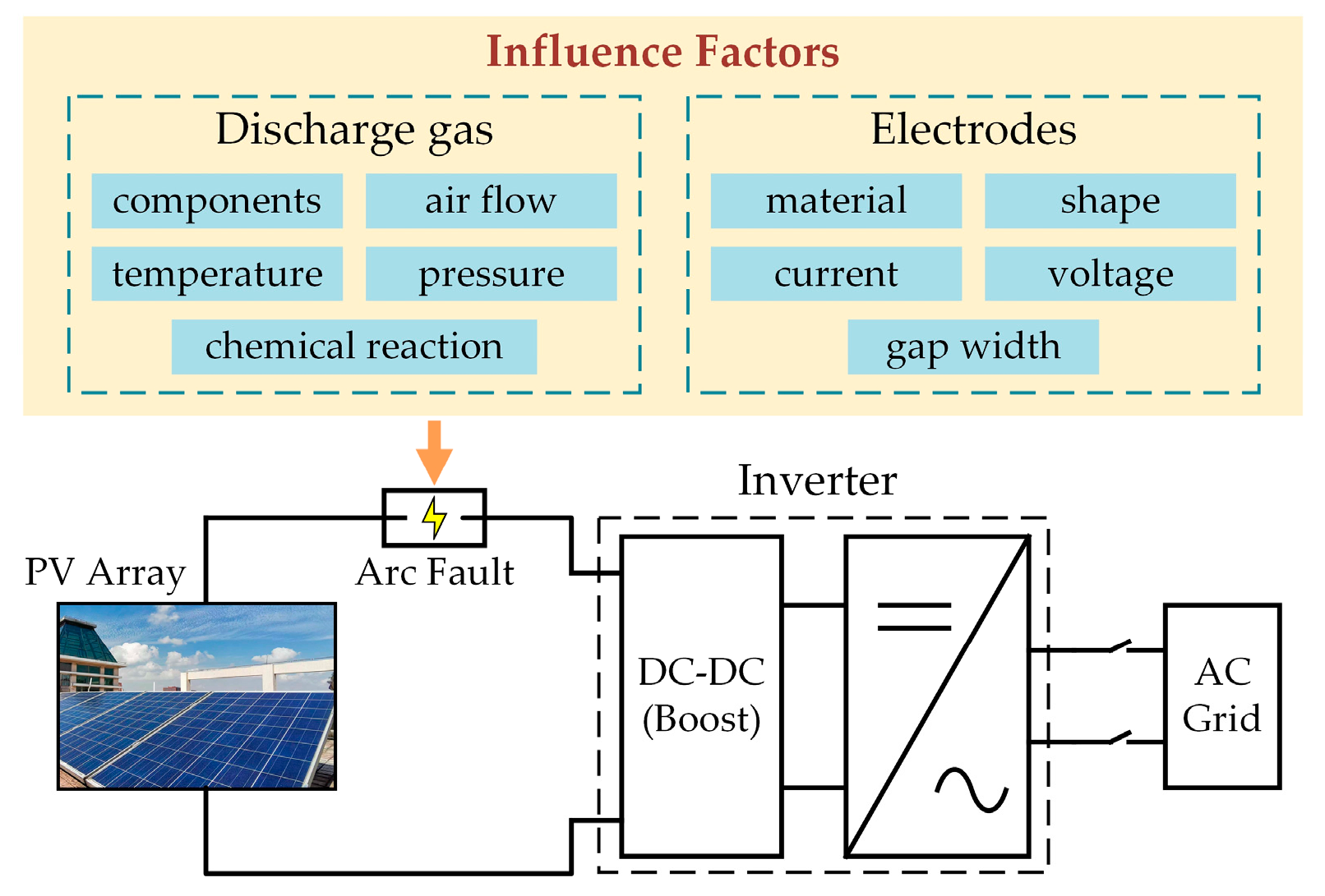
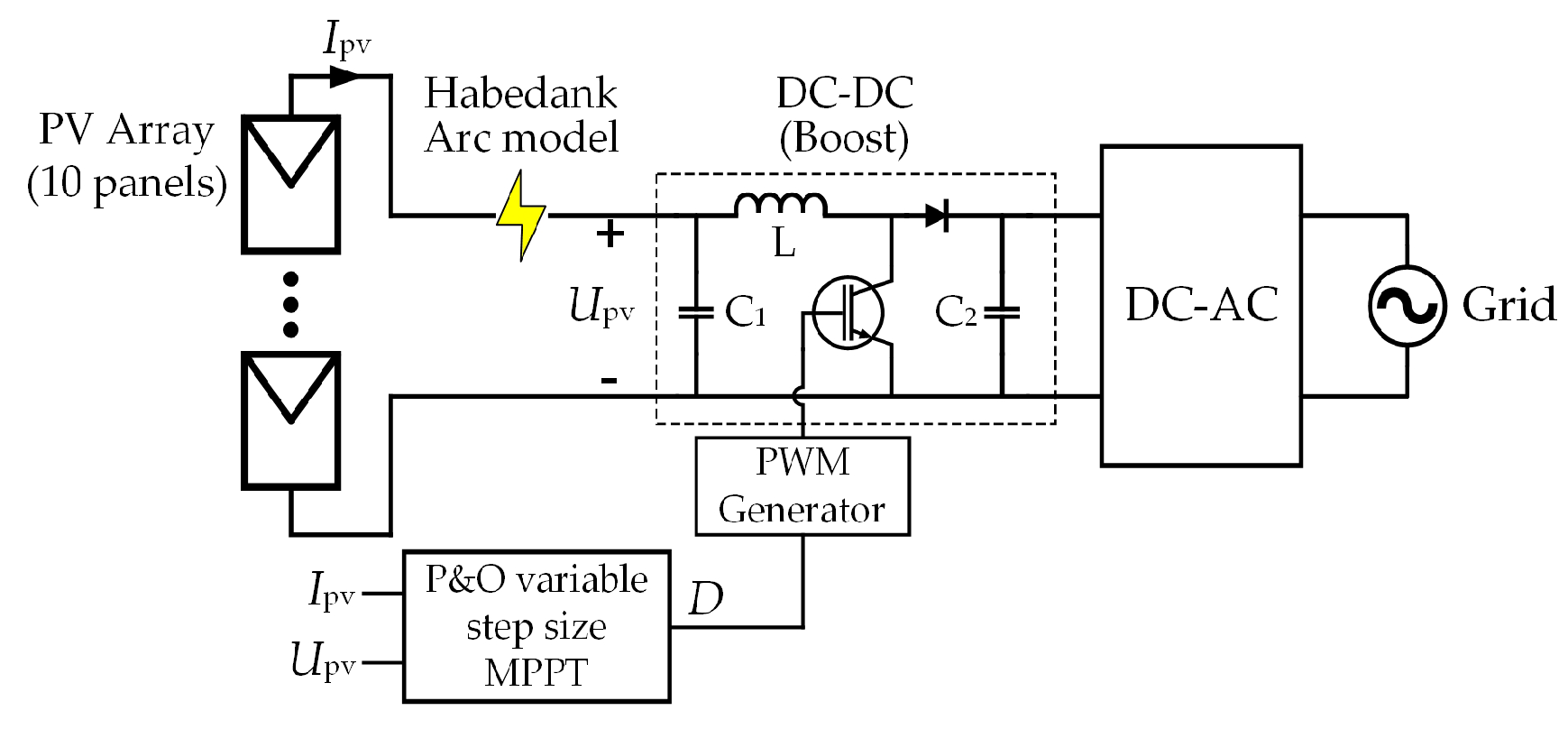
Because of its higher possibility of occurrence than parallel arc [10], series arc was chosen to study here. The experiment was conducted at a small grid-connected PV station. The topology of experimental circuit is shown in Figure 2. The PV array with a single string of 10 solar panels is connected to the grid with the help of a two-stage inverter. A two-stage inverter with boost circuit is usually used in small-scale PV station because the output voltage of PV array needs to be stepped up to meet the grid connection requirement. The series fault arc is generated at the DC bus, therefore, the arc current is equal to the DC bus current.
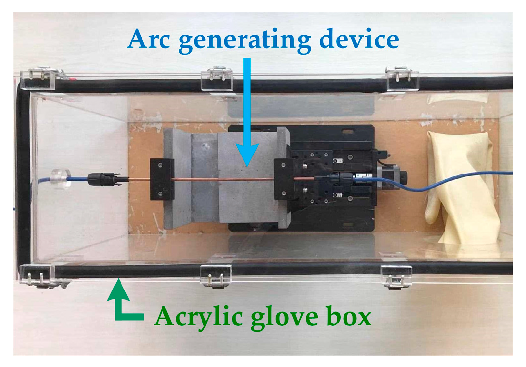
The arc behavior is influenced by the properties of discharge gas and electrodes [35,36,37]. The discharge gas of fault arc is air, which means the gas components, ambient temperature, pressure, and chemical reactions are basically unchanged during the experiment. The electrodes used in the experiment were flat-tip copper columns, which are unified in shape and material. Hence, the airflow and other properties of electrodes, such as current, voltage, and gap width, are the major factors that determine the variations of arcs in the PV system. A flat-tip copper electrode was selected because it can reproduce the characteristics of devices such as connectors that often generate arcs in photovoltaic systems. In Figure 3, an arc-generating platform consisting of an arc-generating device and an acrylic glove box was built, so that the manipulability of experiment could be improved. The fault arcs were generated by separating the electrodes of the arc-generating device. Because the wind will cause the elongation of arc, resulting in a sudden change in the arc voltage [38], a glove box was used to isolate the arc from the outside atmosphere in order to obtain a smooth arc. In addition, the transparent acrylic glove box can provide good observation conditions while blocking splashing combustion. The type of solar panel, inverter, and measuring equipment used in the experiment are shown in Table 1. The parameters of solar panel are given in standard test conditions (1000 W/m2 irradiance, 25 ℃ ambient temperature, and air mass 1.5). The experiments were conducted under uniform irradiance of around 900 W/m2. Besides, six years of operating time attenuates the output of PV array. Therefore, the measured arc current which is equal to the output current of PV array is less than 7.8 A.
3. Arc Fault Signals
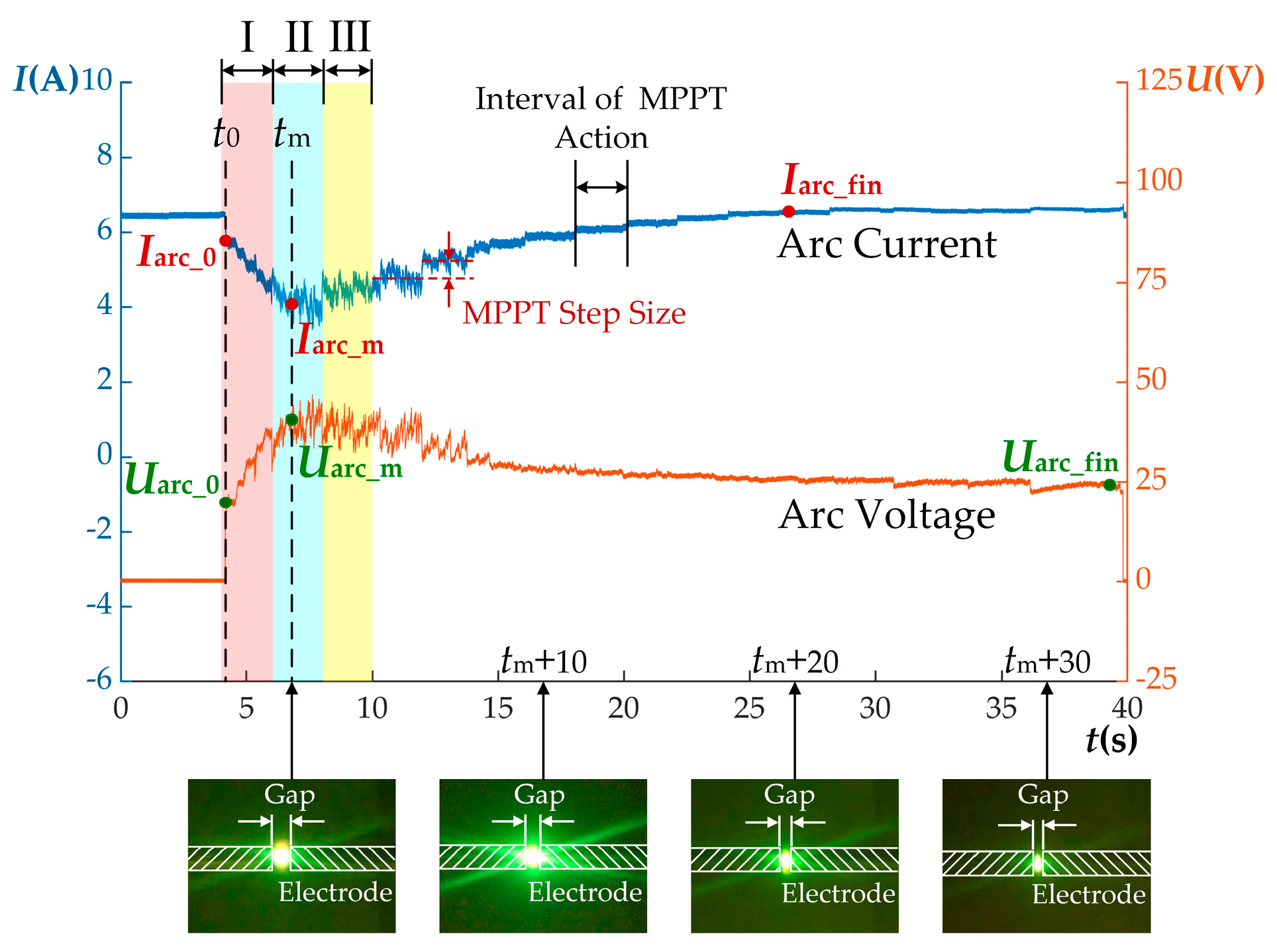
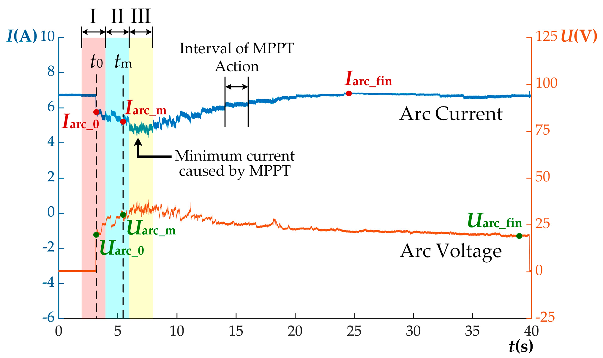
The arc is equivalent to a load in the PV system, and its state is affected by the output of the PV array. In a PV system, the output power of PV array is maximized through MPPT. Thus, the state of the arc is mainly affected by the MPPT under certain environmental conditions (Figure 4). At t0, the arc is generated by separating the two copper electrodes of the arc-generating device. t0 is 0.2 s after the beginning of MPPT period I. The DC bus current which is equal to the arc current steps down to Iarc_0, while the arc voltage steps up to Uarc_0. From t0 to tm, as the gap between the electrodes keeps growing, the arc current therefore continues to decrease, while the arc voltage continues to increase. During this period, the influence of MPPT on the arc is obscured by the intensified arc. At tm, the gap between the electrodes reaches the maximum. As a result, the arc current reaches the minimum value Iarc_m, and the arc voltage reaches the maximum value Uarc_m. During the MPPT period II, the current fluctuation around Iarc_m and the voltage fluctuation around Uarc_m after tm are due to the irregular jumping of the arc.
From MPPT period III, the arc current increases gradually to Iarc_fin in a stepped manner, and the arc voltage decreases gradually to Uarc_fin. Iarc_fin is equal to the DC-link current before the arc occurs. The stair-step arc current waveform is caused by the MPPT action. The width of the step is 2 s, which is equal to the interval of MPPT action. Because the arc voltage is inversely proportional to arc current and proportional to arc length [39], when the arc current increases gradually, the arc voltage decreases correspondingly. Besides, a phenomenon of reduced gap occurs due to the thermal expansion of the electrodes, as shown at the bottom of Figure 4. The gap is photographed every 10 s from tm. Because of the isolation of the glove box, the arc length is approximately equal to the width of the gap. Thus, the arc length decreases as the gap decreases, which results in the decrease of the arc voltage. In summary, the reduction of the arc voltage is caused by increasing arc current and decreasing gap.
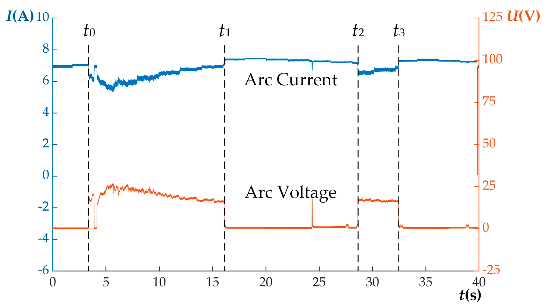
Especially if the gap is too small, the distance between the electrodes will decrease to zero due to the thermal expansion of the electrodes, which means a spontaneous arc-extinguishing situation occurs (Figure 5). The arc is generated at t0. At t1, the two electrodes are in contact because of thermal expansion, and the arc is extinguished. During t1 and t2, without the arc to produce heat, the electrodes gradually cool and contract. At t2, the cooled electrodes separate from each other, and the arc reignites. At t3, the two electrodes contact each other again, causing the arc to extinguish.
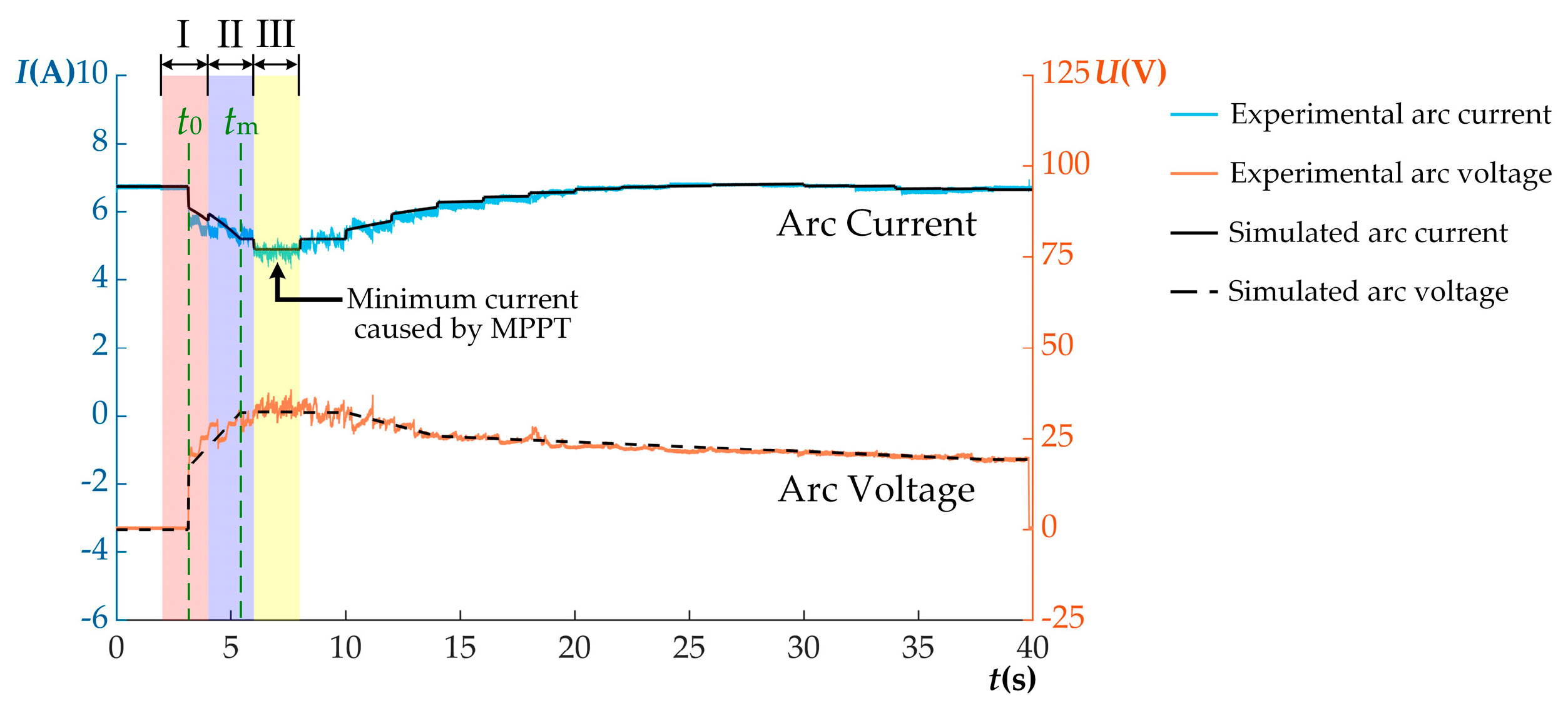
Sometimes, the lowest DC-link current is not caused by the series arc but the action of the MPPT (Figure 6). At tm, the gap between the electrodes reaches the maximum. The arc current should have reached its minimum value in MPPT period II. However, during MPPT period III, the arc current steps down to a lower level due to the negative perturbation of MPPT. In addition, due to the inverse relationship between the arc current and the arc voltage, the arc voltage reaches its maximum value in MPPT period III. The main difference between arc waveforms in Figure 4 and Figure 6 is that the arc current in Figure 4 starts to increase from MPPT period III, while the arc current in Figure 6 continues to decrease. A complete explanation of this phenomenon is shown in Section 6 along with the simulation results.
4. DC Fault Arc Model
Some variables that are crucial to the operation of the PV system are difficult or inconvenient to obtain during the arc-fault experiment, for example, the duty cycle of the boost circuit given by the MPPT algorithm. However, with the help of simulation, all those important variables can be monitored at the same time. The first step to establish an arc-fault PV system is to select an appropriate arc model.
4.1. U–I Arc Model
Since 20th century, many U–I arc models have been developed based on the characteristics of arc voltage, current, and length [39]. The earliest equation for arc modeling was proposed by Ayrton as [40]
where A is the voltage drop of electrodes, B is voltage gradient, C and D are empirical constants, L is arc length, and Uarc and Iarc are arc voltage and current, respectively.
Due to thermal expansion and ablation of electrodes caused by the arc, the variation of electrode gap is nonlinear. Therefore, for long-time arcs, it is difficult to obtain accurate gap width during arcing. In addition, the arc will bend because of the Lorentz force generated by itself [27], so the actual arc length cannot be obtained by simply measuring the electrode gap. As a result, the arc length L or gap width is the major factor that affects the accuracy of the long-time arc simulation using U–I arc models. Other U–I arc models such as Paukert model [41] and Stokes and Oppenlander model [42] also suffer from the same problem.
4.2. Physics-Based Arc Model
The physics-based arc model is also called the arc black box model, which is derived from the principle of energy balance. It has been widely used in simulation or calculation of arc-containing circuits, such as circuit breaker [43,44,45], railway traction system [46], and aircraft power system [47]. The Cassie [48] and Mayr [49] arc models are the most classic black box arc models and are suitable for the simulation of large current and small current arcs, respectively. In order to improve the applicable current range of the arc model, the Habedank arc model considers the arc to be composed of two parts in series, which are described by the Cassie and Mayr arc models, respectively [50]:
where g is arc conductance, i is arc current, gM and gC are conductance described by the Mayr and Cassie arc models respectively, and τM and τC are Mayr and Cassie time constants, respectively, P0 is power loss in Mayr arc model, and UC is arc constant in Cassie arc model. The output current of the PV array is related to solar irradiance and the topology of PV array, meaning the output current varies in a large range. Thus, the Habedank arc model is more suitable to simulate the DC fault arc of different currents than Cassie and Mayr arc models. When applying arc black box models in simulation, the most important and difficult part is the determination of parameters. For arc black box models, the time constant τ only affects how fast the DC arc waveform changes and has no impact on the stable value. The stable value of DC arc waveform is determined by other parameters in the model. Therefore, the determination of τ is less important and difficult than the determination of other parameters. After applying the method in Section 4.3 to Habedank model, only three parameters remain to be determined. And two of the three parameters are time constants τM and τC. Therefore, it gives Habedank model the advantage in parameter determination over other arc black box models, such as Schavemaker model [51] and Schwarz model [52].
Comparisons between Habedank model and other types of models commonly used to simulate the arc are shown in Table 2. Although the arc models based on fundamental physical equations have the advantage of describing the chaotic behavior of the arc, they require high computing power. Approximations have been taken by researchers such as Lowke [53] to reduce the complexity of the physical equations of the arc. Based on simplified physical equations, these arc models can obtain the basic physical quantities of arc, while the complexity is moderate. However, changing arcing conditions, such as nonlinearly varying electrode gap and melting electrodes, make it difficult in determining the boundary conditions of physical equations. Compared with U–I arc models, the parameters of Habedank model do not contain arc length or gap width, which means simulation results will not be affected by inaccurate measurement of arc length and gap width. Therefore, the Habedank model can be selected to simulate long-time DC arc in PV system.
4.3. Parameters Determination of Habedank Arc Model
Unlike alternating current (AC) arc, the current of the DC arc has no zero-crossings. After the DC arc is stable, its conductance is almost constant. Hence, except that τM and τC are empirical values, P0 and UC cannot be determined by the method in [50]. Based on the assumption that gM is equal to gC, a method to determine the parameters of Habedank arc model under steady state is proposed in [54]. However, this assumption is not always satisfied in reality. Thus, a modified method to determine P0 and UC needs to be proposed for the DC arc in PV systems. Since the arc variation time is on the order of microseconds [55], its variation time is negligible compared to the time required for electrode expansion and interval of MPPT action. Therefore, if small variation caused by irregular jumping of arc is ignored, the change of arc can be regarded as a transient state, during which the conductance of the arc is constant. Thus, the conductance described in the Habedank arc model can be presented as the following equation:
By substituting (3) into (2), the following equation can be obtained:
By assuming , where α is a positive constant, the following equation can be deduced:
Finally, by substituting (5) into (4), parameter P0 and UC can be described by the following equation:
where u is arc voltage. As a result, P0 can be regarded as the function of α, u, and i. And UC can be regarded as the function of α and u.
When calculating P0 and UC according to Equation (6), the variation of arc current i and voltage u is simplified as linear. Figure 4 is taken as an example to illustrate: From t0 to tm, the arc current decreases linearly from Iarc_0 to Iarc_m, while the arc voltage increases from Uarc_0 to Uarc_m. From MPPT period III, the arc current increases linearly to Iarc_fin, while the arc voltage decreases to Uarc_fin. The advantage of this method is that only a few special moments of arc current and voltage values are required. Moreover, the process of determining parameters P0 and UC is simplified to determine the value of α.
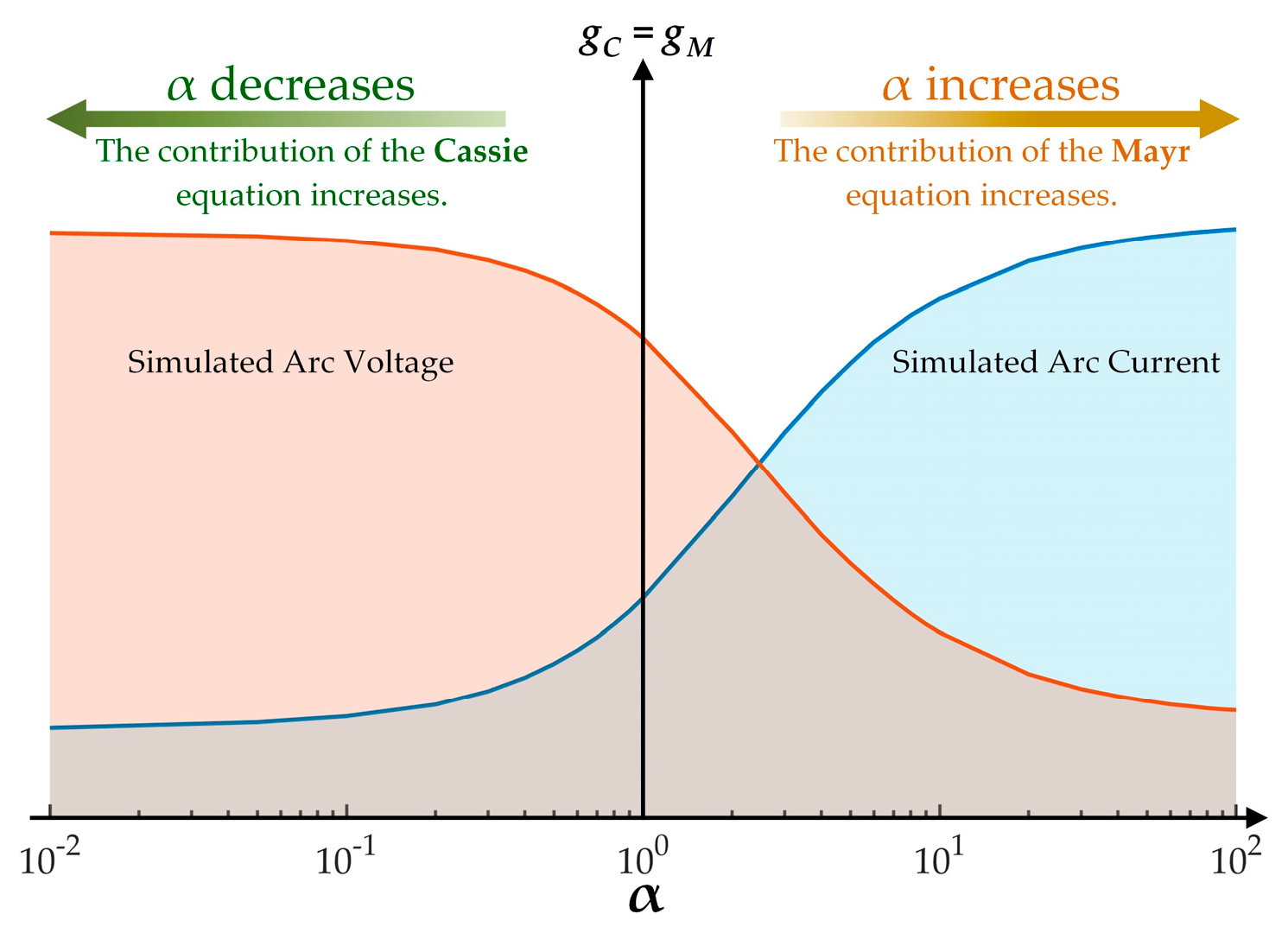
After u and i are determined for calculation, different α will result in different simulated arc currents and voltages (Figure 7). When α = 1, the contribution of the Cassie and Mayr equation to the Habedank arc model are the same. As α decreases, the simulated arc current increases, while the simulated arc voltage decreases, and the contribution of the Cassie equation increases. On the contrary, when α increases, the contribution of the Mayr equation increases. Therefore, according to this relationship between α and arc current and voltage, an appropriate value of α can be obtained when the differences between simulation results and experimental data reach the minimum.
5. Model Validation
5.1. Simulation Setup
According to the experimental circuit, a simulation circuit including Habedank arc model and PV system was built in MATLAB/Simulink (Figure 8). In the boost circuit, the input capacitor C1 and output capacitor C2 are decoupling capacitors used for mitigating the power fluctuation effect at the PV-array side and balancing the power between DC side and AC side, respectively [56]. Ipv and Upv are the output current of PV array and the voltage on the input side of boost circuit, respectively. D is the duty cycle of the boost circuit.
A variable-step-size MPPT based on the P&O algorithm was adapted in simulation to maintain the maximum output of the PV array [57]. The duty cycle D is determined by the MPPT algorithm. Table 3 shows the arc model parameters setting of the arc waveforms in Figure 4 and Figure 6. The mean values of arc current and voltage were used in simulation when calculating P0 and UC.
5.2. Simulation Results
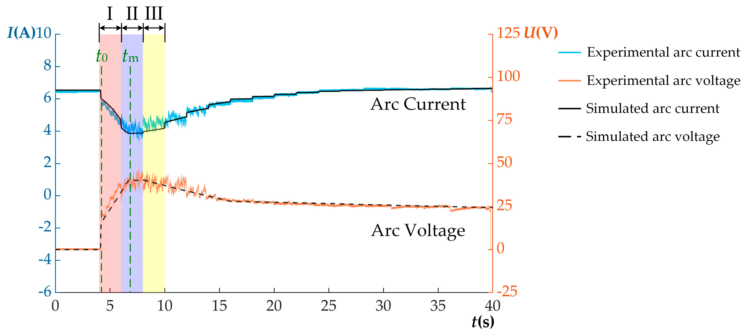
The simulation results of experimental arc waveforms in Figure 4 and Figure 6 are shown in Figure 9 and Figure 10 respectively. Although the proposed model cannot describe chaotic variations of the arc current and voltage, the trends of all simulation waveforms are consistent with the experimental waveforms. The simulated arc current waveforms have the same step-like changes as the experimental waveforms after tm.
Equations used to calculate the signed relative error (SRE) of the simulation results are shown as follows:
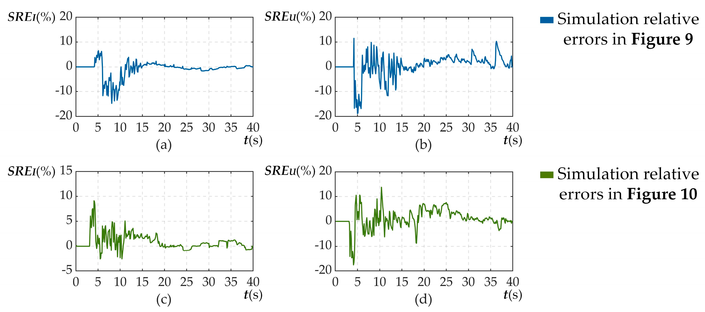
where SREI and SREU are SREs of the simulated arc current and the simulated arc voltage, respectively; Ie and Is are measured and simulated arc currents, respectively; and Ue and Us are arc voltages obtained by experiment and simulation, respectively. The positive or negative of SER reflects the position of the simulated waveforms relative to the experimental waveforms; that is, a positive SRE indicates that the simulated waveform is above the experimental waveform, while a negative SRE means the simulated waveform is below the experimental waveform. The SREs of simulation results are shown in Figure 11, where the SREs are calculated every 0.1 s.
Despite the impact of external airflow on the arc being minimized by the utilization of glove box, the arc still represented chaotic behaviors including elongation, shortening, and spot motion. These dynamic movements are mainly caused by Lorentz force generated by the arc and electrodes [58,59], resulting in the fluctuation of arc voltage. Thus, the experimental voltage waveforms fluctuate around the simulated voltage waveforms, which causes the positive and negative alternation of SREU. As the gap between the electrodes decreases after tm, the variation of the arc length decreases relatively, the absolute value of SREU therefore decreases correspondingly. Because of the inverse relationship between the arc current and arc voltage, SREI and SREU change in opposite directions, which can be better observed in MPPT period I, II, and III. Although the maximum mismatches of simulated arc current and voltage reach 14.8% and 18.6% respectively, there is good correlation between the simulation results and the measured ones with adjusted R-squared from 0.946 to 0.956. The adjusted R-squared is a statistics measure that represents the correlation between simulation results and experimental values. A comparison between the simulation results and the ones in other references is shown in Table 4. It shows that the proposed model is competitive to other models.
6. Discussion
In the previous section, the validity of the proposed simulation system is verified. It is difficult to understand the interactions between the arc variation and MPPT action from the experimental data. However, these complicated interactions can be well analyzed with the help of simulation.
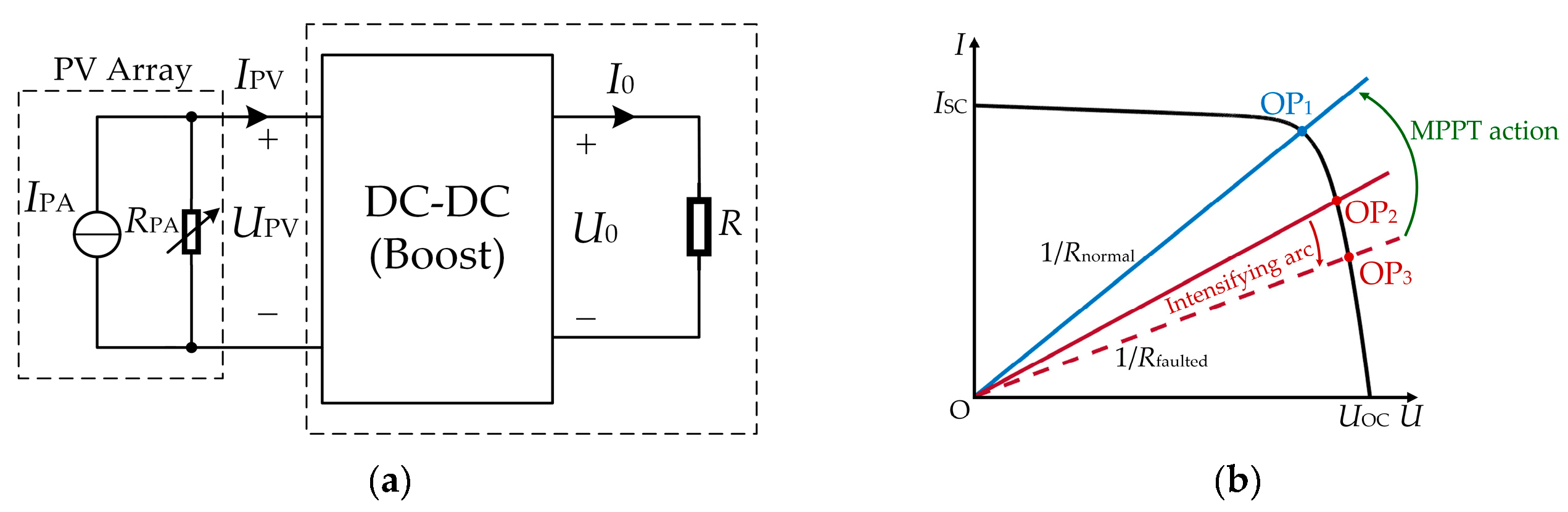
The main difference between the simulated arc waveforms in Figure 9 and Figure 10 is that the arc current in Figure 10 drops to a lower level in MPPT period III, while the arc current in Figure 9 does not. Before further explanation, it is necessary to understand how MPPT maintains the maximum output of PV array (Figure 12a). The PV array can be simplified to a current source IPA connected to a variable resistance RPA in parallel, and the load is simplified as a constant resistance R. For a boost circuit, the following equations can be obtained:
where U0 and I0 are the output voltage and output current of the boost circuit, respectively. Thus, the equivalent resistance of the external circuit without arc (Rnormal) can be derived as follows:
The output power of PV array (PPA) can be obtained as:
When Rnormal is equal to RPA, the PV array has the maximum output power. Therefore, MPPT can achieve the maximum power point (MPP) of PV array by controlling D.
For a PV array under certain irradiance and temperature, its operation point (OP) is the intersection point of its U–I curve, and the line with a slope of 1/Req, where Req is the equivalent resistance of the external circuit (Figure 12b). In a nonfault condition, the OP1 oscillates in a very small range around MPP. When an arc occurs at the DC bus, the OP jumps from OP1 to OP2, causing the voltage of PV array to step up. The equivalent resistance of the external circuit when arc happens (Rfaulted) can be obtained as:
where the Rarc is the arc resistance. As the gap between the electrodes increases, the Rarc increases correspondingly; therefore, the OP gradually moves from OP2 to OP3. In order to move the OP from OP3 to MPP, the duty cycle D must be increased to reduce the Rfaulted to Rnormal.
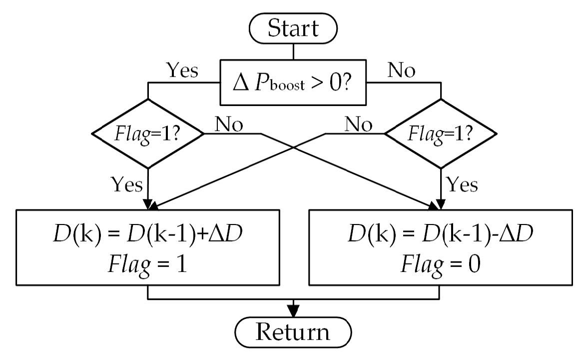
Since the increase and decrease of D are controlled by MPPT algorithm, the variation of arc current in both experiment and simulation can be explained by the judgements of MPPT algorithm under arc-fault state. The flowchart of P&O algorithm used in the simulation is shown in Figure 13, where the ∆Pboost is the variation of the input power of the boost circuit, and ∆D is the variable step of the MPPT algorithm. The variable Flag has two values, 0 and 1, which refer to the negative and positive perturbations of MPPT, respectively. A negative perturbation indicates a decrease in D, while a positive perturbation indicates an increase in D. When entering a new MPPT period, Ipv and Upv will be first sampled, and then the MPPT algorithm will determine the variation of D according to the sign of ∆Pboost and the value of Flag in the previous MPPT period.
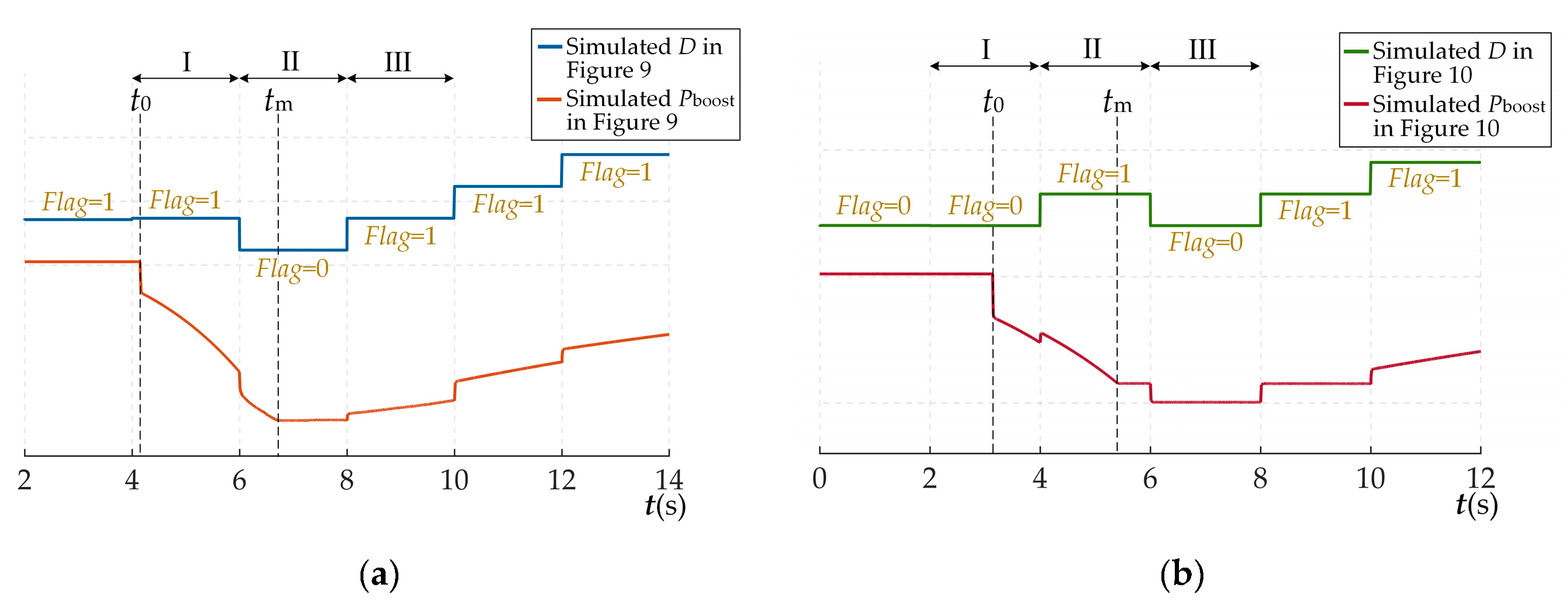
When P&O algorithm is selected as the MPPT algorithm, the variations of D and Pboost are shown in Figure 14. From t0 to tm, due to the intensifying arc, the Pboost drops down gradually, leading to a negative ∆Pboost. Thus, in MPPT periods II and III, the variation of D is opposite to that of the previous MPPT period, according to Figure 13. As discussed above, in order to increase the output of PV array, D must be increased. Hence, from MPPT period II, the decrease of D, which is a negative perturbation of MPPT, moves the OP further away from OP1, resulting in the decrease of arc current, Pboost, and the output power of PV array. In Figure 14a, the P&O algorithm keeps D increasing from MPPT period III, causing the OP to move towards OP1 and the arc current to increase. The occurrence of negative perturbation is in the same MPPT period as the moment when the electrode gap reaches maximum. Therefore, the minimum value of the simulated arc current appears in MPPT period II. In Figure 14b, the negative perturbation of MPPT occurs in MPPT period III, causing the OP to move further away from OP1. As a result, the arc current and Pboost drop down to a lower level.
In summary, the influence of MPPT on the arc is that the arc current changes in a stair-step manner from MPPT period III. The arc can also affect the MPPT through negative perturbations. Under arc-fault condition, the negative perturbations of MPPT decrease the output power of the PV array, which is the opposite of the purpose of MPPT. Besides, the negative perturbation also affects the change of arc current. That is, if Flag is equal to 0 at tm, the arc current Iarc will start to increase in the next MPPT period. On the contrary, if Flag is equal to 1 at tm, a lower Iarc will appear in the next MPPT period due to the negative perturbation.
7. Conclusions
This paper has introduced a method to simulate the long-time-series DC arc in a PV system using MATLAB/Simulink software. The Habedank model was selected to simulate the U–I characteristics of the long-time DC arc, because it is not affected by the varying gap width, its parameters are simple to determine, and the computing power requirement is low. And the parameters determination process of Habedank model under the condition of long-time DC arc was introduced. Then, a PV system based on a P&O MPPT algorithm was combined with the Habedank model for long-time DC arc simulation under uniform irradiance. The simulation results show good correlation with the measured data. Finally, based on the simulation results, the interactions between the arc and MPPT were investigated. It shows that the arc can cause the P&O MPPT algorithm to reduce the output power of PV array through negative perturbation of MPPT, while the MPPT can influence the change of arc current.
In order to have a preliminary understanding of complex interactions between the arc and PV system, this study was conducted under uniform irradiance, which is the simplest situation. However, there are many complicated situations in reality. Therefore, the following research should be carried out in the future: (1) the interactions between DC arc and PV system under varying irradiance; (2) the impact of DC arc on advanced MPPT algorithms, such as global maximum power point tracking algorithms; (3) methods to enhance the robustness of MPPT algorithms under arc-fault conditions; (4) the impact of arcs of different types and locations on PV systems.
Author Contributions
Conceptualization: X.L. and Y.S.; methodology: X.L. and C.P.; software: X.L., D.L., and Y.S.; validation: X.L.; writing—original draft preparation: X.L. and C.P.; writing—review and editing, X.L., D.L., and Y.S.; supervision: Y.S.; project administration: X.L. and Y.S. All authors have read and agreed to the published version of the manuscript.
Funding
This research was funded by the National Key Research and Development Program of China (Grant No. 2018YFB1500904 and No. 2019YFB2103200). It was also funded by the National Natural Science Foundation of China (Grant No. 61374129).
Conflicts of Interest
The authors declare no conflict of interest.
References
- Hastings, J.K.; Juds, M.A.; Luebke, C.J.; Pahl, B. A Study of Ignition Time for Materials Exposed to DC Arcing in PV Systems. In Proceedings of the 2011 37th IEEE Photovoltaic Specialists Conference (PVSC), Seattle, WA, USA, 19–24 June 2011. [Google Scholar]
- Haeberlin, H. Arc Detector as an External Accessory Device for PV Inverters for Remote Detection of Dangerous Arcs on the DC Side of PV Plants. In Proceedings of the European Photovoltaic Solar Energy Conference, Valencia, Spain, Citeseer, 6–10 September 2010. [Google Scholar]
- NFPA 70: National Electrical Code; National Fire Protection Association: Quincy, MA, USA, 2011.
- UL 1699b. Outline of Investigation for Photovoltaic (PV) DC Arc-Fault Circuit Protection; Underwriters Laboratories: Northbrook, IL, USA, 2011. [Google Scholar]
- Xiong, Q.; Ji, S.C.; Zhu, L.Y.; Zhong, L.; Liu, Y. A Novel DC Arc Fault Detection Method Based on Electromagnetic Radiation Signal. IEEE Trans. Plasma Sci. 2017, 45, 472–478. [Google Scholar] [CrossRef]
- Miao, W.C.; Liu, X.Y.; Lam, K.H.; Pong, P.W.T. DC-Arcing Detection by Noise Measurement With Magnetic Sensing by TMR Sensors. IEEE Trans. Magn. 2018, 54, 5. [Google Scholar] [CrossRef]
- Johnson, J.; Pahl, B.; Luebke, C.; Pier, T.; Miller, T.; Strauch, J.; Kuszmaul, S.; Bower, W. Photovoltaic DC arc fault detector testing at Sandia National Laboratories. In Proceedings of the 2011 37th IEEE Photovoltaic Specialists Conference, IEEE, Seattle, WA, USA, 19–24 June 2011; pp. 003614–003619. [Google Scholar]
- Johnson, J.; Montoya, M.; Mccalmont, S.; Katzir, G.; Fuks, F.; Earle, J.; Fresquez, A.; Gonzalez, S.; Granata, J. Differentiating Series and Parallel Photovoltaic Arc-Faults. In Proceedings of the 2012 38th IEEE Photovoltaic Specialists Conference, Austin, TX, USA, 3–8 June 2012; pp. 720–726. [Google Scholar]
- Gao, Y.; Zhang, J.; Lin, Y.; Sun, Y. An Innovative Photovoltaic DC Arc Fault Detection Method through Multiple Criteria Algorithm Based on a New Arc Initiation Method. In Proceedings of the 2014 IEEE 40th Photovoltaic Specialist Conference (PVSC), Denver, CO, USA, 8–13 June 2014; pp. 3188–3192. [Google Scholar]
- Chen, S.L.; Li, X.W.; Xiong, J.Y. Series Arc Fault Identification for Photovoltaic System Based on Time-Domain and Time-Frequency-Domain Analysis. IEEE J. Photovolt. 2017, 7, 1105–1114. [Google Scholar] [CrossRef]
- He, C.X.; Mu, L.H.; Wang, Y.J. The Detection of Parallel Arc Fault in Photovoltaic Systems Based on a Mixed Criterion. IEEE J. Photovolt. 2017, 7, 1717–1724. [Google Scholar] [CrossRef]
- Yao, X.; Herrera, L.; Ji, S.C.; Zou, K.; Wang, J. Characteristic Study and Time-Domain Discrete-Wavelet-Transform Based Hybrid Detection of Series DC Arc Faults. IEEE Trans. Power Electron. 2014, 29, 3103–3115. [Google Scholar] [CrossRef]
- Zhu, H.; Wang, Z.; Balog, R.S. Real Time arc Fault Detection in PV Systems Using Wavelet Decomposition. In Proceedings of the 2016 IEEE 43rd Photovoltaic Specialists Conference (PVSC), Portland, OR, USA, 5–10 June 2016; pp. 1761–1766. [Google Scholar]
- Xiong, Q.; Feng, X.Y.; Gattozzi, A.L.; Liu, X.; Zheng, L.; Zhu, L.; Ji, S.; Hebner, R.E. Series Arc Fault Detection and Localization in DC Distribution System. IEEE Trans. Instrum. Meas. 2020, 69, 122–134. [Google Scholar] [CrossRef]
- Gao, Y.; Dong, J.; Sun, Y.; Lin, Y.; Zhang, R. PV Arc-Fault Feature Extraction and Detection Based on Bayesian Support Vector Machines. Int. J. Smart Grid Clean Energy SGCE 2015, 4, 283–290. [Google Scholar] [CrossRef] [Green Version]
- Wang, Z.; Balog, R.S. Arc Fault and Flash Detection in Photovoltaic Systems Using Wavelet Transform and Support Vector Machines. In Proceedings of the 2016 IEEE 43rd Photovoltaic Specialists Conference, Portland, OR, USA, 5–10 June 2016; pp. 3275–3280. [Google Scholar]
- Yi, Z.; Etemadi, A. Line-to-Line Fault Detection for Photovoltaic Arrays Based on Multi-resolution Signal Decomposition and Two-stage Support Vector Machine. IEEE Trans. Ind. Electron. 2017, 64, 8546–8556. [Google Scholar] [CrossRef]
- Grichting, B.; Goette, J.; Jacomet, M. Cascaded Fuzzy Logic based Arc Fault Detection in Photovoltaic Applications. In Proceedings of the 2015 International Conference on Clean Electrical Power (ICCEP), Taormina, Italy, 16–18 June 2015; pp. 178–183. [Google Scholar]
- Telford, R.D.; Galloway, S.; Stephen, B.; Elders, I. Diagnosis of Series DC Arc Faults-A Machine Learning Approach. IEEE Trans. Ind. Inform. 2017, 13, 1598–1609. [Google Scholar] [CrossRef] [Green Version]
- Alam, M.K.; Khan, F.H.; Johnson, J.; Flicker, J. PV Arc-fault Detection using Spread Spectrum Time Domain Reflectometry (SSTDR). In Proceedings of the 2014 IEEE Energy Conversion Congress and Exposition, Pittsburgh, PA, USA, 14–18 September 2014; pp. 3294–3300. [Google Scholar]
- Georgijevic, N.L.; Jankovic, M.V.; Srdic, S.; Radakovic, Z. The Detection of Series Arc Fault in Photovoltaic Systems Based on the Arc Current Entropy. IEEE Trans. Power Electron. 2016, 31, 5917–5930. [Google Scholar] [CrossRef]
- Ahmadi, M.; Samet, H.; Ghanbari, T. A New Method for Detecting Series Arc Fault in Photovoltaic Systems Based on the Blind-Source Separation. IEEE Trans. Ind. Electron. 2020, 67, 5041–5049. [Google Scholar] [CrossRef]
- Gleizes, A.; Gonzalez, J.J.; Freton, P. Thermal plasma modelling. J. Phys. D-Appl. Phys. 2005, 38, R153–R183. [Google Scholar] [CrossRef]
- Li, X.W.; Chen, D.G.; Li, R.; Wu, Y.; Niu, C. Electrode Evaporation Effects on Air Arc Behavior. Plasma Sci. Technol. 2008, 10, 323–327. [Google Scholar]
- Li, M.; Wu, Y.; Wu, Y.; Liu, Y.; Hu, Y. MHD Modeling of Fault Arc in a Closed Container. IEEE Trans. Plasma Sci. 2014, 42, 2714–2715. [Google Scholar] [CrossRef]
- Rong, M.Z.; Yang, F.; Wu, Y.; Murphy, A.B.; Wang, W.; Guo, J. Simulation of Arc Characteristics in Miniature Circuit Breaker. IEEE Trans. Plasma Sci. 2010, 38, 2306–2311. [Google Scholar] [CrossRef]
- Rau, S.H.; Zhang, Z.Y.; Lee, W.J. 3-D Magnetohydrodynamic Modeling of DC Arc in Power System. IEEE Trans. Ind. Appl. 2016, 52, 4549–4555. [Google Scholar] [CrossRef]
- Flicker, J.; Johnson, J. Electrical Simulations of Series and Parallel PV Arc-Faults. In Proceedings of the 2013 IEEE 39th Photovoltaic Specialists Conference, Tampa, FL, USA, 16–21 June 2013; pp. 3165–3172. [Google Scholar]
- Yao, X.; Herrera, L.; Wang, J. Impact Evaluation of Series DC Arc Faults in DC Microgrids. In Proceedings of the 2015 Thirtieth Annual IEEE Applied Power Electronics Conference and Exposition, Charlotte, NC, USA, 15–19 March 2015; pp. 2953–2958. [Google Scholar]
- Uriarte, F.M.; Gattozzi, A.L.; Herbst, J.D.; Estes, H.B.; Hotz, T.J.; Kwasinski, A.; Hebner, R.E. A DC Arc Model for Series Faults in Low Voltage Microgrids. IEEE Trans. Smart Grid 2012, 3, 2063–2070. [Google Scholar] [CrossRef]
- Wang, Z.; Balog, R.S. Arc Fault and Flash Signal Analysis in DC Distribution Systems Using Wavelet Transformation. IEEE Trans. Smart Grid 2015, 6, 1955–1963. [Google Scholar] [CrossRef]
- Chen, S.L.; Li, X.W.; Xie, Z.M.; Meng, Y. Time-Frequency Distribution Characteristic and Model Simulation of Photovoltaic Series Arc Fault With Power Electronic Equipment. IEEE J. Photovolt. 2019, 9, 1128–1137. [Google Scholar] [CrossRef]
- Dhar, S.; Dash, P.K. Differential Current-Based Fault Protection with Adaptive Threshold for Multiple PV-Based DC Microgrid. IET Renew. Power Gener. 2017, 11, 778–790. [Google Scholar] [CrossRef]
- Ahmadi, M.; Samet, H.; Ghanbari, T. Series Arc Fault Detection in Photovoltaic Systems Based on Signal-to-Noise Ratio Characteristics Using Cross-Correlation Function. IEEE Trans. Ind. Inform. 2020, 16, 3198–3209. [Google Scholar] [CrossRef]
- Chapman, S.; Cowling, T.G.; Burnett, D. The Mathematical Theory of Non-Uniform Gases: An Account of the Kinetic Theory of Viscosity, Thermal Conduction and Diffusion in Gases; Cambridge University Press: Cambridge, UK, 1990. [Google Scholar]
- Paschen, F. Ueber die zum Funkenübergang in Luft, Wasserstoff und Kohlensäure bei verschiedenen Drucken erforderliche Potentialdifferenz. Ann. Phys. 1889, 273, 69–96. [Google Scholar] [CrossRef]
- Johnson, J.; Armijo, K. Parametric Study of PV Arc-Fault Generation Methods and Analysis of Conducted DC Spectrum. In Proceedings of the 2014 IEEE 40th Photovoltaic Specialist Conference (PVSC), Denver, CO, USA, 8–13 June 2014; pp. 3543–3548. [Google Scholar]
- Kizilcay, M.; Pniok, T. Digital-Simulation of Fault Arcs in Power-Systems. Eur. Trans. Electr. Power Eng. 1991, 1, 55–60. [Google Scholar] [CrossRef]
- Ammerman, R.F.; Gammon, T.; Sen, P.K.; Nelson, J.P. DC-Arc Models and Incident-Energy Calculations. IEEE Trans. Ind. Appl. 2010, 46, 1810–1819. [Google Scholar] [CrossRef]
- Ayrton, H. The mechanism of the Electric Arc. Philos. Trans. R. Soc. Lond. A Contain. Pap. Math. Phys. Character 1902, 199, 299–336. [Google Scholar]
- Paukert, J. The Arc Voltage and Arc Resistance of LV Fault Arcs. In Proceedings of the 7th International conference on Switching Arc Phenomena, Lodz, Poland, 27 September–1 October 1993; pp. 49–51. [Google Scholar]
- Stokes, A.D.; Oppenlander, W.T. Electric-Arcs in Open Air. J. Phys. D Appl. Phys. 1991, 24, 26–35. [Google Scholar] [CrossRef]
- Pinto, L.C.; Zanetta, L.C. Medium Voltage SF6 Circuit-Breaker Arc Model Application. Electr. Power Syst. Res. 2000, 53, 67–71. [Google Scholar] [CrossRef]
- Chang, G.W.; Huang, H.M.; Lai, J.H. Modeling SF6 Circuit Breaker for Characterizing Shunt Reactor Switching Transients. IEEE Trans. Power Deliv. 2007, 22, 1533–1540. [Google Scholar] [CrossRef]
- Ohtaka, T.; Kerterz, V.; Smeets, R.P.P. Novel Black-Box Arc Model Validated by High-Voltage Circuit Breaker Testing. IEEE Trans. Power Deliv. 2018, 33, 1835–1844. [Google Scholar] [CrossRef]
- Liu, Y.J.; Chang, G.W.; Huang, H.M. Mayr’s Equation-Based Model for Pantograph Arc of High-Speed Railway Traction System. IEEE Trans. Power Deliv. 2010, 25, 2025–2027. [Google Scholar] [CrossRef]
- Jiang, Y.; Wu, J.W.; Jia, B.W. Reignition After Interruption of Intermediate-Frequency Vacuum Arc in Aircraft Power System. IEEE Access 2018, 6, 8649–8656. [Google Scholar]
- Cassie, A.M. Arc Rupture and Circuit Severity: A New Theory. In Proceedings of the Conférence Internationale des Grands Réseaux Électriques à Haute Tension (CIGRE Report), Paris, France, 29 June–8 July 1939; Volume 102, pp. 1–14. [Google Scholar]
- Mayr, O. Beiträge zur Theorie des Statischen und des Dynamischen Lichtbogens. Arch. Elektr. 1943, 37, 588–608. [Google Scholar] [CrossRef]
- Habedank, U. Application of a New Arc Model for the Evaluation of Short-Circuit Breaking Tests. IEEE Trans. Power Deliv. 1993, 8, 1921–1925. [Google Scholar] [CrossRef]
- Schavemaker, P.H.; van der Sluis, L. An Improved Mayr-Type Arc Model Based on Current-Zero Measurements. IEEE Trans. Power Deliv. 2000, 15, 580–584. [Google Scholar] [CrossRef]
- Schwarz, J. Dynamisches Verhalten Eines Gasbeblasenen, Turbulenzbestimmten Schaltlichtbogens. ETZ-A 1971, 92, 389–391. [Google Scholar]
- Lowke, J.J. Simple Theory of Free-Burning ARCS. J. Phys. D Appl. Phys. 1979, 12, 1873–1886. [Google Scholar] [CrossRef]
- Ju, M.H.; Wang, L. Arc Fault Modeling and Simulation in DC System Based on Habedank Model. In Proceedings of the 2016 Prognostics and System Health Management Conference, Chengdu, China, 19–21 October 2016; Zuo, M.J., Xing, L., Li, Z., Tian, Z., Miao, Q., Eds.; IEEE: New York, NY, USA, 2016. [Google Scholar]
- Ferguson, D.C.; Hoffmann, R.C.; Plis, E.; Engelhart, D. Arc Plasma Propagation and Arc Current Profiles. IEEE Trans. Plasma Sci. 2019, 47, 3842–3847. [Google Scholar] [CrossRef]
- Hu, H.B.; Harb, S.; Kutkut, N.; Batarseh, I.; Shen, Z.J. A Review of Power Decoupling Techniques for Microinverters With Three Different Decoupling Capacitor Locations in PV Systems. IEEE Trans. Power Electron. 2013, 28, 2711–2726. [Google Scholar] [CrossRef]
- Serrano-Guerrero, X.; González-Romero, J.; Cárdenas-Carangui, X.; Escrivá-Escrivá, G. Improved Variable Step Size P&O MPPT Algorithm for PV Systems. In Proceedings of the 2016 51st International Universities Power Engineering Conference (UPEC), Coimbra, Portugal, 6–9 September 2016. [Google Scholar]
- Ghorui, S.; Sahasrabudhe, S.N.; Murthy, P.S.S.; Das, A.K.; Venkatramani, N. Experimental Evidence of Chaotic Behavior in Atmospheric Pressure Arc Discharge. IEEE Trans. Plasma Sci. 2000, 28, 253–260. [Google Scholar] [CrossRef]
- Tanaka, S.; Matsumura, T. Characteristic dynamic behavior of dc arc near graphite bar electrodes with short gap. J. Appl. Phys. 2001, 89, 4247–4254. [Google Scholar] [CrossRef]
- Zhang, Z.; Nie, Y.; Lee, W.-J. Approach of Voltage Characteristics Modeling for Medium-Low-Voltage Arc Fault in Short Gaps. IEEE Trans. Ind. Appl. 2018, 55, 2281–2289. [Google Scholar] [CrossRef]
- Wu, Z.; Wu, G.; Dapino, M.; Pan, L.; Ni, K. Model for Variable-Length Electrical Arc Plasmas under AC Conditions. IEEE Trans. Plasma Sci. 2015, 43, 2730–2737. [Google Scholar]
Figure 1.
Direct current (DC) fault arc classifications in a photovoltaic (PV) system.

Figure 2.
The topology of experimental circuit and influence factors of arcing.

Figure 3.
Arc generating platform.

Figure 4.
Typical arc voltage and current waveform changes under the action of maximum power point tracking (MPPT) and reduced gap due to the thermal expansion of the electrodes.
Figure 4.
Typical arc voltage and current waveform changes under the action of maximum power point tracking (MPPT) and reduced gap due to the thermal expansion of the electrodes.

Figure 5.
Spontaneous arc-extinguishing phenomenon due to thermal expansion of electrodes.

Figure 6.
Minimum arc current and maximum arc voltage caused by MPPT.

Figure 7.
The influence of α on the simulated arc current and arc voltage when and are constant.

Figure 8.
Simulation circuit.

Figure 9.
Simulation results of arc waveforms in Figure 4.
Figure 9.
Simulation results of arc waveforms in Figure 4.

Figure 10.
Simulation results of arc waveforms in Figure 6.
Figure 10.
Simulation results of arc waveforms in Figure 6.

Figure 11.
Signed relative errors of simulation results: (a) relative error of simulated arc current in Figure 9; (b) relative error of simulated arc voltage in Figure 9; (c) relative error of simulated arc current in Figure 10; (d) relative error of simulated arc voltage in Figure 10.

Figure 12.
(a) Simplified circuit of PV system with MPPT and (b) the changes of PV array operation point in arc-fault condition.
Figure 12.
(a) Simplified circuit of PV system with MPPT and (b) the changes of PV array operation point in arc-fault condition.

Figure 13.
Flowchart of the perturb & observation (P&O) algorithm.

Figure 14.
When P&O is selected as the MPPT algorithm, the variations of simulated D and Pboost in (a) Figure 9 and (b) Figure 10.


Table 1.
Experiment conditions.
| Solar Panel Type | Maximum Power Point | Short-Circuit Current | Open-Circuit Voltage |
| JT240PLe | (7.8 A, 30.8 V) | 8.55 A | 37.2 V |
| Inverter | Oscillator | Current Probe | Voltage Probe |
| Zeverlution3000S | Tektronix MSO2024 | Tektronix TCP0030 | Sapphire SI-9110 |
Table 2.
Characteristics of different types of arc models.
| Model | Advantage | Computing Power Requirement |
|---|---|---|
| U–I arc model | Easy to build the model | Low |
| Habedank model | No need to measure the arc length and gap width | Low |
| Arc models based on simplified physical equations | The basic physical quantities of arc can be obtained, while the complexity is moderate. | Low to medium |
| Arc models based on fundamental physical equations | Describe the chaotic behavior of arc | High |
© 2020 by the authors. Licensee MDPI, Basel, Switzerland. This article is an open access article distributed under the terms and conditions of the Creative Commons Attribution (CC BY) license (http://creativecommons.org/licenses/by/4.0/).
Share and Cite
MDPI and ACS Style
Li, X.; Pan, C.; Luo, D.; Sun, Y. Series DC Arc Simulation of Photovoltaic System Based on Habedank Model. Energies 2020, 13, 1416. https://doi.org/10.3390/en13061416
AMA Style
Li X, Pan C, Luo D, Sun Y. Series DC Arc Simulation of Photovoltaic System Based on Habedank Model. Energies. 2020; 13(6):1416. https://doi.org/10.3390/en13061416
Chicago/Turabian StyleLi, Xinran, Chenyun Pan, Dongmei Luo, and Yaojie Sun. 2020. "Series DC Arc Simulation of Photovoltaic System Based on Habedank Model" Energies 13, no. 6: 1416. https://doi.org/10.3390/en13061416
Note that from the first issue of 2016, this journal uses article numbers instead of page numbers. See further details here.