Designs of Feedback Controllers for Fluid Flows Based On Model Predictive Control and Regression Analysis

Abstract

Complexity of online computation is a drawback of model predictive control (MPC) when applied to the Navier–Stokes equations. To reduce the computational complexity, we propose a method to approximate the MPC with an explicit control law by using regression analysis. In this paper, we extracted two state-feedback control laws and two output-feedback control laws for flow around a cylinder as a benchmark. The state-feedback control laws that feed back different quantities to each other were extracted by ridge regression, and the two output-feedback control laws, whose measurement output is the surface pressure, were extracted by ridge regression and Gaussian process regression. In numerical simulations, the state-feedback control laws were able to suppress vortex shedding almost completely. While the output-feedback control laws could not suppress vortex shedding completely, they moderately improved the drag of the cylinder. Moreover, we confirmed that these control laws have some degree of robustness to the change in the Reynolds number. The computation times of the control input in all the extracted control laws were considerably shorter than that of the MPC.

1. Introduction

To improve fuel efficiency and reducing emission of greenhouse gas, many studies on suppression of flow separation [1,2] and turbulence [3] by adding a small amount of control actuation to flow have been done. In most of these studies, open-loop control, where the control action is determined regardless of the state of flow, is employed. However, closed-loop control, where the control action is determined based on information about a flow field from sensors, has recently been paid attention with the remarkable development of sensors and actuators. Although applications are still limited to relatively slow flows, the closed-loop control of fluid flows is actually realized in some experiments [4,5,6,7,8,9,10,11,12]. In general, the closed-loop control is expected to improve the regulation performance, robustness against the changes in the environment, and energy efficiency.

A wide variety of feedback control methods has been examined for fluid flows so far. For examples, there are heuristic methods based on experiments or simulation results [4,5,6,7,8,13], adaptive control [9,10,11,12], and linear optimal control [14,15,16,17]. In this paper, we focus on model predictive control (MPC), which is based on the nonlinear optimal control theory. In the literature, there have been applications of MPC to turbulence flow [18], thermal fluid flow [19], and flow around a circular cylinder [20,21,22]. The advantage of MPC over other methods is that control laws can be designed in consideration of flow nonlinearities and actuator constraints.

In MPC, the control input is obtained by solving optimal control problems on a finite future time interval repeatedly. Only the first portion of each optimal control input is applied to the system to be controlled at each time. Hence, this control law has a local time optimality. Optimal control problems cannot be solved explicitly in general, especially for nonlinear systems, and they are normally solved numerically. Thus, MPC involves online optimization. This fact leads to a well-known drawback of MPC. Namely, it requires a huge amount of computational cost. Due to this computational complexity of online optimization, it is difficult to implement MPC in actual control systems for fluid flow.

Against the problem on computational complexity inherent in MPC, we propose a method to design control laws that imitate MPC. The first step of the proposed method is collection of a large amount of data of the flow field and the control input obtained by numerical simulations of closed-loop control using MPC. The simulations require a high computational cost, but they are carried out offline. To design a control law, we assume that there is an unknown functional relationship between the data of flow field and the data of the control input generated by MPC. Then, a control law is learned based on the data by means of the regression analysis. The obtained control laws are not computationally expensive because they do not require online optimization.

Our approach is similar to the one proposed by Mathelin et al. [23]. In their approach, the data of the optimal control input is acquired by solving the optimal control problems for the reduced-order model. Then, the control law is extracted from the data by polynomial approximation based on the projection. One of the main differences between our approach and the one of Mathelin et al., is the model assumed in the optimal control problem. They used the reduced-order model whereas we use the full-order model, that is the Navier–Stokes equations. Therefore, the control input used as teaching data in our approach is optimal for the full-order fluid model. Although some sophisticated approaches for model reduction have been proposed [24,25,26], the approximation accuracy of the resulting optimal control input is not mathematically guaranteed. In addition, the use of regression analysis is one of the features of our approach. Although the potential of regression analysis has been mentioned in [23], the polynomial approximation was mainly used. Since the dimension of state variables in full-state models is quite high, it is difficult to use polynomial approximation based on the projection. Regression analysis enables us to extract control laws even from high-dimensional data.

Our preliminary result has been reported in the conference paper [27]. A control law was designed for flow around a circular cylinder by the proposed method as a benchmark problem. It is common in the field of fluid-flow control to deal with flow around a cylinder as a benchmark problem. Applications of control methods to flow around a cylinder include passive control [28], reinforcement learning control [29], and suboptimal control [30]. In our previous paper, a relatively slow flow at Reynolds number $Re=100$ was considered. At this level of Reynolds number, laminar flow separation occurs on the cylinder surface, and alternating vortex shedding appears behind. The control objective was to suppress vortex shedding by manipulating magnitude of two jets coming out of the cylinder surface independently. We designed an output-feedback control law that uses pressure distribution on the cylinder surface based on the Gaussian process regression. Although improvement of aerodynamic performance was observed when the proposed control law was applied to the flow, the performance was clearly less effective than the actual MPC. This is an unsurprising consequence because MPC results in a state feedback control law. Hence, a fair evaluation of the effectiveness of the proposed method explained in the previous paragraph was not conducted.

In this paper, we consider almost the same control problem as the one in our conference paper [27]. There are substantial differences in the paper. The total mass flow rate of two manipulated jets in almost zero. This assumption makes it more difficult to suppress the vortex shedding. To evaluate the effectiveness of our proposed approach appropriately, state-feedback control laws are designed first. In addition, we employ the degree of asymmetry of the flow as a cost functional associated with the optimal control problem in MPC. The viscous dissipation was used in [27]. Our new choice results in a slightly simple optimal control problem. We will observe that state feedback control laws extracted with linear regression provides an almost the same performance as MPC without much computational cost. An output feedback control law is designed based on Gaussian process regression. To extract another output-feedback control law, we also use linear regression for comparison with Gaussian process regression. This is devoted to clarifying the capability of our proposed approach. Furthermore, we examine robustness of the extracted control laws to slight changes in the Reynolds number.

This paper is organized as follows: In Section 2 we design model predictive controller for flow around a cylinder and then in Section 2 show application results in a numerical simulation. Section 4 provides the proposed methods to design two state-feedback control laws and two output-feedback control laws for flow around a cylinder. Then, in Section 5 the four control laws are designed for the flow at $Re=100$. They are applied to the flows at different Reynolds number including $Re=100$. Some conclusions are mentioned in Section 6.

2. Design of Model Predictive Controller

2.1. Model Predictive Control for Finite Dimensional Systems

Before applying MPC to flow around a cylinder, we explain MPC for finite dimensional systems in order that readers can grasp the concept of MPC. Let us consider the following finite dimensional system:

$$\begin{array}{cc}\hfill & \dot{\mathbf{X}}\left(t\right)=f(\mathbf{X}\left(t\right),\mathbf{V}\left(t\right)),0<t<\infty ,\hfill \end{array}$$

(1)

$$\begin{array}{cc}\hfill & \mathbf{X}\left(0\right)={\mathbf{X}}_0,\hfill \end{array}$$

(2)

where $t\in \mathbb{R}$, $\mathbf{V}\left(t\right)\in {\mathbb{R}}^{N_V}$, $\mathbf{X}\left(t\right)\in {\mathbb{R}}^{N_X}$, and ${\mathbf{X}}_0\in {\mathbb{R}}^{N_X}$ are the time variable, the control input, the state variable, and the initial state, respectively for some $N_X,N_V\in \mathbb{N}$. In MPC for the system (1) and (2), the control input is determined by solving the following optimal control problem at each time:

$$\begin{array}{cc}\hfill & \mathrm{Find}{\overline{\mathbf{V}}}^{*}=\underset{\overline{\mathbf{V}}}{\arg \min }J[\overline{\mathbf{X}},\overline{\mathbf{V}}]\hfill \\ \hfill & \mathrm{s}.\mathrm{t}.\hfill \end{array}$$

(3)

$$\begin{array}{cc}\hfill & \dot{\overline{\mathbf{X}}}\left(\tau \right)=f(\overline{\mathbf{X}}\left(\tau \right),\overline{\mathbf{V}}\left(\tau \right)),t<\tau <t+T,\hfill \end{array}$$

(4)

$$\begin{array}{cc}\hfill & \overline{\mathbf{X}}\left(t\right)=\mathbf{X}\left(t\right),\hfill \end{array}$$

(5)

where $\tau \in \mathbb{R}$, $\overline{\mathbf{X}}\left(\tau \right)\in {\mathbb{R}}^{N_X}$, and $\overline{\mathbf{V}}\left(\tau \right)\in {\mathbb{R}}^{N_V}$ are the time variable, the state variable, and the control input in the optimal control problem, respectively. The functional $J[\overline{\mathbf{X}},\overline{\mathbf{V}}]\in \mathbb{R}$ is a performance index. The performance index J is designed so that minimizing it implies the achievement of a control objective.

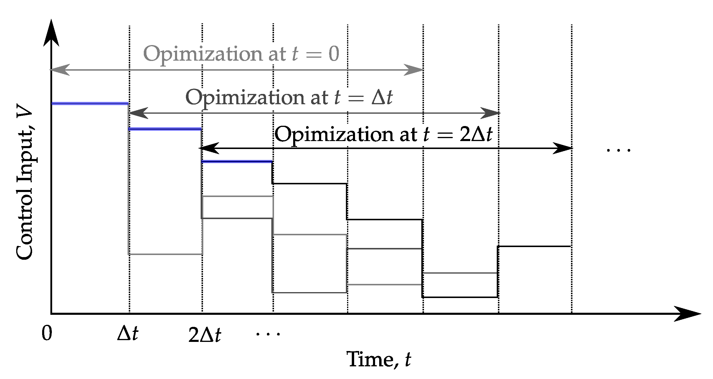
Once the state $X\left(t\right)$ in the actual system is measured at some time t, we can predict the future behavior of the system on the interval $[t,t+T]$ from Equations (4) and (5). The model predictive controller employs the predicted behavior that minimizes the performance index and computes the optimal control input to achieve it. Then, only the first portion of the optimal control input ${\overline{\mathbf{V}}}^{*}\left(\tau \right),(t<\tau <t+\mathsf{\Delta }t)$ is applied to the actual system. After $t+\mathsf{\Delta }t$, we measure the state of the actual system, compute the optimal control input, and apply it to the system again. This cycle is iterated in the MPC. Figure 1 shows the relationship between the optimal control input and the control input applied to the system in the MPC. The horizon where optimization is done moves forward as time advances.

2.2. Model Predictive Control for Flow around a Cylinder

We design a model predictive controller for flow around a cylinder. First, we determine an optimal control problem by modeling the flow and setting a performance index. Next, we represent adjoint equations which are necessary to numerically solve the optimal control problem. To simplify the notation, this subsection does not distinguish between the notation of variables in the actual system and variables in the optimal control problem, except for the time variables t and $\tau$.

2.2.1. State Equations

An overall view and an enlarged view of the spatial domain considered in this paper are shown in Figure 2a,b. If we assume that the fluid in the domain is incompressible, the dynamic behavior of the flow is described by the following Navier–Stokes and continuity equations:

$$\begin{array}{cc}\frac{\partial \mathbf{u}}{\partial \tau }+\nabla ·(\mathbf{u}\otimes \mathbf{u})=-\nabla p+\frac{1}{Re}{\nabla }^2\mathbf{u},& \mathrm{in}\mathsf{\Omega }\times (t,t+T),\end{array}$$

(6)

$$\begin{array}{cc}\hfill \nabla ·\mathbf{u}& =0,\mathrm{in}\mathsf{\Omega }\times (t,t+T),\hfill \end{array}$$

(7)

where $Re\in \mathbb{R}$ is the free stream Reynolds number, $\mathsf{\Omega }\subset {\mathbb{R}}^2$ is the annulus domain surrounding the cylinder, $T\in \mathbb{R}$ is the length of the prediction horizon, and ⊗ denotes the outer product. The flow velocity vector $\mathbf{u}(\mathbf{x},\tau )={[u_1(\mathbf{x},\tau ),u_2(\mathbf{x},\tau )]}^{\mathsf{T}}\in {\mathbb{R}}^2$, the pressure $p(\mathbf{x},t)\in \mathbb{R}$, the spatial variable $\mathbf{x}={[x_1,x_2]}^{\mathsf{T}}\in {\mathbb{R}}^2$, and the time variables $t\in \mathbb{R}$ and $\tau \in \mathbb{R}$ are non-dimensionalized. The reference quantities are the free stream velocity, the cylinder diameter, and the fluid density.

We regard mean velocity of jets emitted from small areas on the surface as the manipulated variable $U\left(\tau \right)\in \mathbb{R}$. We assume that the radial velocity on the small areas ${\mathsf{\Gamma }}_{\mathrm{c},1}$ and ${\mathsf{\Gamma }}_{\mathrm{c},2}$ is proportional to the manipulated variable, and the velocity takes zero on the surface excluding ${\mathsf{\Gamma }}_{\mathrm{c},1}$ and ${\mathsf{\Gamma }}_{\mathrm{c},2}$. These are formulated as a boundary condition on the surface as follows:

$$\begin{array}{c}\hfill \mathbf{u}(\mathbf{x},\tau )=\left\{\begin{array}{c}U\left(\tau \right)f_{\mathrm{p},1}\left(\mathbf{x}\right)\mathbf{n}\left(\mathbf{x}\right),\mathrm{on}{\mathsf{\Gamma }}_{\mathrm{c},1}\times (t,t+T),\hfill \\ -U\left(\tau \right)f_{\mathrm{p},2}\left(\mathbf{x}\right)\mathbf{n}\left(\mathbf{x}\right),\mathrm{on}{\mathsf{\Gamma }}_{\mathrm{c},2}\times (t,t+T),\hfill \\ \mathbf{0},\mathrm{on}{\mathsf{\Gamma }}_{\backslash c}\times (t,t+T),\hfill \end{array}\right.\end{array}$$

(8)

where $\mathbf{n}\left(\mathbf{x}\right)\in {\mathbb{R}}^2$ is the outer unit normal vector, and ${\mathsf{\Gamma }}_{\backslash \mathrm{c}}$ is the area excluding ${\mathsf{\Gamma }}_{\mathrm{c},1}$ and ${\mathsf{\Gamma }}_{\mathrm{c},2}$ from the cylinder surface. The functions $f_{\mathrm{p},1}\left(\mathbf{x}\right)\in \mathbb{R}$ and $f_{\mathrm{p},2}\left(\mathbf{x}\right)\in \mathbb{R}$ represent velocity profiles like the Hagen-Poiseuille flow. If we denote the sizes of small areas by $|{\mathsf{\Gamma }}_{\mathrm{c},1}|$ and $|{\mathsf{\Gamma }}_{\mathrm{c},2}|$, the profiles $f_{\mathrm{p},1}\left(\mathbf{x}\right)$ and $f_{\mathrm{p},2}\left(\mathbf{x}\right)$ satisfy the following normalization conditions:

$$\begin{array}{c}\hfill \frac{1}{|{\mathsf{\Gamma }}_{\mathrm{c},1}|}{\int }_{{\mathsf{\Gamma }}_{\mathrm{c},1}}{f}_{\mathrm{p},1}\left(\mathbf{x}\right)d\mathbf{x}=\frac{1}{|{\mathsf{\Gamma }}_{\mathrm{c},2}|}{\int }_{{\mathsf{\Gamma }}_{\mathrm{c},2}}{f}_{\mathrm{p},2}\left(\mathbf{x}\right)d\mathbf{x}=1.\end{array}$$

(9)

This normalization conditions are necessary so that $U\left(\tau \right)$ is the mean velocity of the jets. Equation (8) is common impervious and non-slip boundary condition except the existence of the jets. The physical meaning of (8) is that there are two injection holes on the cylinder surface, and when fluid is sucked into one hole, fluid is emitted out from the other hole as shown in Figure 2a,b. Moreover, the magnitude of the inflow and outflow from the two holes are same.

In order to facilitate implementation of control laws, the manipulated variable $U\left(\tau \right)$ is discretized in time using the first-order hold:

$$\begin{array}{cc}\hfill \dot{U}& =V_n,t+(n-1)\mathsf{\Delta }t<\tau <t+n\mathsf{\Delta }t,n=1,2,\dots ,N,\hfill \end{array}$$

(10)

$$\begin{array}{cc}\hfill U& =U_t,\mathrm{at}\{\tau =t\},\hfill \end{array}$$

(11)

where $U_t\in \mathbb{R}$ is the mean velocity of the two jets measured at time t, and $\mathsf{\Delta }t\in \mathbb{R}$ is the control cycle. The time derivative of the jet velocity $V_n\in \mathbb{R}$ is the control input, and it is treated as the decision variable in the optimal control problem.

It is assumed that on ${\mathsf{\Gamma }}_{\mathrm{in}}$, the left portion of the outer circle of the annulus $\mathsf{\Omega }$, the magnitude of the velocity is constant, and it is directed to the right:

$$\begin{array}{c}\hfill \mathbf{u}={[1,0]}^{\mathsf{T}},\mathrm{on}{\mathsf{\Gamma }}_{\mathrm{in}}\times (t,t+T).\end{array}$$

(12)

On the right semicircle ${\mathsf{\Gamma }}_{\mathrm{out}}$, the following homogeneous Neumann boundary condition is imposed on the velocity vector:

$$\begin{array}{c}\hfill \nabla \mathbf{u}·\mathbf{n}=0,\mathrm{on}{\mathsf{\Gamma }}_{\mathrm{out}}\times (t,t+T).\end{array}$$

(13)

The boundary conditions (12) and (13) mean that fluid flows in from the left of the domain $\mathsf{\Omega }$ and flows out to the right.

The initial condition of the velocity vector in the optimal control problem is

$$\begin{array}{c}\hfill \mathbf{u}={\mathbf{u}}_t,\mathrm{on}\mathsf{\Omega }\times \{\tau =t\},\end{array}$$

(14)

where ${\mathbf{u}}_t\left(\mathbf{x}\right)\in {\mathbb{R}}^2$ is the velocity vector measured at the real time t.

2.2.2. Cost Functional

Vortex shedding of flow over a cylinder is characterized by asymmetry of the velocity vector field. Naturally, the vortex shedding can be suppressed by weakening the asymmetry of the flow. Therefore, in the performance index, we evaluate the asymmetry function defined by the following equation:

$$\begin{array}{c}\hfill {\mathsf{\Phi }}_{\mathrm{Asym}}\left(\tau \right)={\int }_{\mathsf{\Omega }}\left\{{\left(u_1(x_1,x_2,\tau )-u_1(x_1,-x_2,\tau )\right)}^2+{\left(u_2(x_1,x_2,\tau )+u_2(x_1,-x_2,\tau )\right)}^2\right\}d\mathbf{x}.\end{array}$$

(15)

The asymmetry function ${\mathsf{\Phi }}_{\mathrm{Asym}}\left(\tau \right)$ is nonnegative, and it takes zero if the rightward flow velocity distribution $u_1$ is symmetric and the upward flow velocity distribution $u_2$ is antisymmetric about the $x_1$ axis.

Using ${\mathsf{\Phi }}_{\mathrm{Asym}}\left(\tau \right)$, we set the performance index as follows:

$$\begin{array}{c}\hfill \frac{1}{2}{\int }_t^{t+T}{U}^2\left(\tau \right)d\tau +\frac{Q_1}{2}\sum _{n=1}^N{V}_n^2+Q_2{\mathsf{\Phi }}_{\mathrm{Asym}}(t+T),\end{array}$$

(16)

where $Q_1\in \mathbb{R}$ and $Q_2\in \mathbb{R}$ are the positive weight coefficients. The first term of (16) evaluates the magnitude of jet speed, the second term evaluates the magnitude of the rate of the change in the jet velocity, and the third term evaluates the asymmetry of the flow field. The control law minimizing the cost functional (16) is expected to suppress the asymmetry with small control effort.

2.2.3. Adjoint Equations

Optimal control problem we consider is the problem of finding the sequence of control input $V_n,(n=1,2,\dots ,N)$ that minimizes the cost functional (16) subject to (6)–(14). Although this minimization problem is the complicated problem whose constraints are partial differential equations, necessary conditions for the minimization can be derived using the calculus of variations. The derivation of the necessary conditions can be found in Appendix A. If we introduce the adjoint variables $\mathbf{v}(\mathbf{x},\tau )={[v_1(\mathbf{x},\tau ),v_2(\mathbf{x},\tau )]}^{\mathsf{T}}\in {\mathbb{R}}^2$, $q(\mathbf{x},\tau )\in \mathbb{R}$, and $\lambda \left(\tau \right)\in \mathbb{R}$, we have the following necessary conditions from the stationary condition of a Lagrangian composed of the cost functional (16) and the constraints (6)–(14):

$$\begin{array}{cc}\frac{\partial \mathbf{v}}{\partial \tau }+\mathbf{u}·\left(\nabla \mathbf{v}+\nabla {\mathbf{v}}^{\mathsf{T}}\right)+\nabla \mathbf{q}+\frac{1}{Re}{\nabla }^2\mathbf{v}=0,& \mathrm{in}\mathsf{\Omega }\times (t,t+T),\end{array}$$

(17)

$$\begin{array}{cc}\nabla ·\mathbf{v}=0,& \mathrm{in}\mathsf{\Omega }\times (t,t+T),\end{array}$$

(18)

$$\begin{array}{cc}\hfill \mathbf{v}=0,\mathrm{on}({\mathsf{\Gamma }}_{\mathrm{in}}+& {\mathsf{\Gamma }}_{\mathrm{c},1}+{\mathsf{\Gamma }}_{\mathrm{c},2}+{\mathsf{\Gamma }}_{\backslash \mathrm{c}})\times (t,t+T),\hfill \end{array}$$

(19)

$$\begin{array}{cc}\left\{\mathbf{v}\otimes \mathbf{u}+\nabla \mathbf{v}+(\mathbf{v}·\mathbf{u}+q)I\right\}·\mathbf{n}=0,& \mathrm{on}{\mathsf{\Gamma }}_{\mathrm{out}}\times (t,t+T),\end{array}$$

(20)

$$\begin{array}{ccc}& \hfill \mathbf{v}·\mathbf{n}=0,& \mathrm{on}{\mathsf{\Gamma }}_{\mathrm{out}}\times (t,t+T),\\ \hfill -\dot{\lambda }+U+\left\{{\int }_{{\mathsf{\Gamma }}_{c,1}}\left(\mathbf{n}·\nabla \mathbf{v}·\mathbf{n}+q\right)f_{\mathrm{p},1}d\mathbf{x}\right.& & \end{array}$$

(21)

$$\begin{array}{cc}\left.-{\int }_{{\mathsf{\Gamma }}_{c,2}}\left(\mathbf{n}·\nabla \mathbf{v}·\mathbf{n}+q\right)f_{\mathrm{p},1}d\mathbf{x}\right\}=0,& \mathrm{on}(t,t+T),\end{array}$$

(22)

$$\begin{array}{cc}\mathbf{v}+2Q_2\left(\mathbf{u}-\tilde{\mathbf{u}}\right)=0,& \mathrm{on}\mathsf{\Omega }\times \{\tau =t+T\},\end{array}$$

(23)

$$\begin{array}{cc}\lambda =0,& \mathrm{at}\{\tau =t+T\},\end{array}$$

(24)

$$\begin{array}{cc}{Q}_2{V}_n-{\int }_{(n-1)\mathsf{\Delta }t}^{n\mathsf{\Delta }t}\lambda d\tau =0,& n=1,2,\dots ,N,\end{array}$$

(25)

where $\tilde{\mathbf{u}}(\mathbf{x},\tau )={[u_1(x_1,-x_2,\tau ),-u_2(x_1,-x_2,\tau )]}^{\mathsf{T}}\in {\mathbb{R}}^2$ is the flow velocity vector distribution obtained by reflecting $\mathbf{u}(\mathbf{x},\tau )$ with respective to the $x_1$ axis. Equations (17) and (22) are time evolution equations for the adjoint variables, (18) is a static constraint equation, (19)–(21) are adjoint boundary conditions, and (23) and (24) are terminal conditions. The left-hand side of (25) is the gradient of the cost functional with respect to the control input $V_n$ under the constraints (6)–(14). Once the adjoint variable $\lambda \left(\tau \right)$ is obtained by solving the state Equations (6)–(14) and the adjoint Equations (17)–(24), we can evaluate the left-hand side of (25). Hence, we can numerically compute the gradient of cost functional with respect to $V_n$ in the following procedure:

• Solve the state Equations (6)–(14) from $\tau =t$ to $\tau =t+T$ with a certain sequence of the control input $V_n,(n=1,2,\cdots ,N)$.
• Solve the adjoint Equations (17)–(24) backward from $\tau =t+T$ to $\tau =t$ with the use of the states $\mathbf{u}(\mathbf{x},\tau )$ and $U\left(\tau \right)$ obtained in Step 1.
• Compute the left-hand side of (25) by using $\lambda \left(\tau \right)$ obtained in Step 2 and $V_n$ employed in Step 1.

If the gradient information of the cost functional is available, we can apply gradient-based optimization algorithms such as the gradient descent method to find the numerical solution to the optimal control problem.

3. Numerical Simulations of Model Predictive Control

We apply MPC to flow around a circular cylinder at $Re=100$ in this section. First, we explain the methods for optimization and numerical simulations, and then discuss the results of applying MPC.

3.1. Numerical Methods

We use the quasi-Newton method for solving the optimal control problem. The quasi-Newton method has better convergence speed near the optimal solution than the gradient descent method [31]. An approximated Hessian matrix in the quasi-Newton method is updated by the BFGS (Broyden-Fletcher-Goldfarb-Shanno) method. Optimal solutions are found in the iterative procedure, and we end the iteration when the $l_2$-norm of the gradient of the cost functional falls below ${10}^{-3}$.

The SMAC (Simplified Maker and Cell) method, which is a scheme for incompressible fluid, is used for the numerical simulation of the flow. In the SMAC method, the error growth of the continuity equation is prevented by introducing staggered grids. The low-storage third-order Runge-Kutta method combined with the Crank-Nicolson method [32] is used in temporal discretization of the Navier–Stokes equations. Spatial discretization is implemented by the second-order central difference.

The O-type grid is used, and the diameter of the outer boundary circle is 30 times larger than that of the cylinder. The numbers of grid points are $91\times 256$ in the radial and circumference directions, respectively. The grid size in the radial direction gradually decreases as it approaches the cylinder. In order to capture the sharp change in the flow velocity, the minimum grid size near the cylinder surface is set to $0.005$, which is $1/100$ of the $99\%$ boundary layer thickness.

3.2. Results and Discussion

We assume that the state variable in the whole domain is available for computing the control input.

Table 1. Parameters for the controlled system and the model predictive controller.

Parameter	Value
Reynolds Number $Re$	100
width of jet holes $|{\mathsf{\Gamma }}_{\mathrm{c},1}|$, $|{\mathsf{\Gamma }}_{\mathrm{c},2}|$	0.515
weight coefficient $Q_1$	0.2
weight coefficient $Q_2$	0.01
predictive horizon T	6
control cycle $\mathsf{\Delta }{t}_{\mathrm{s}}$	0.3

shows the parameters for the controlled system and the model predictive controller. The two jet holes are attached to the top and bottom of the cylinder, and their size is $8.2\%$ of the entire circumference of the cylinder. The length of the prediction horizon is set to be approximately equal to the cycle of vortex shedding. The control cycle is set to $0.3$, which is approximately $1/20$ of the cycle of vortex shedding without control.

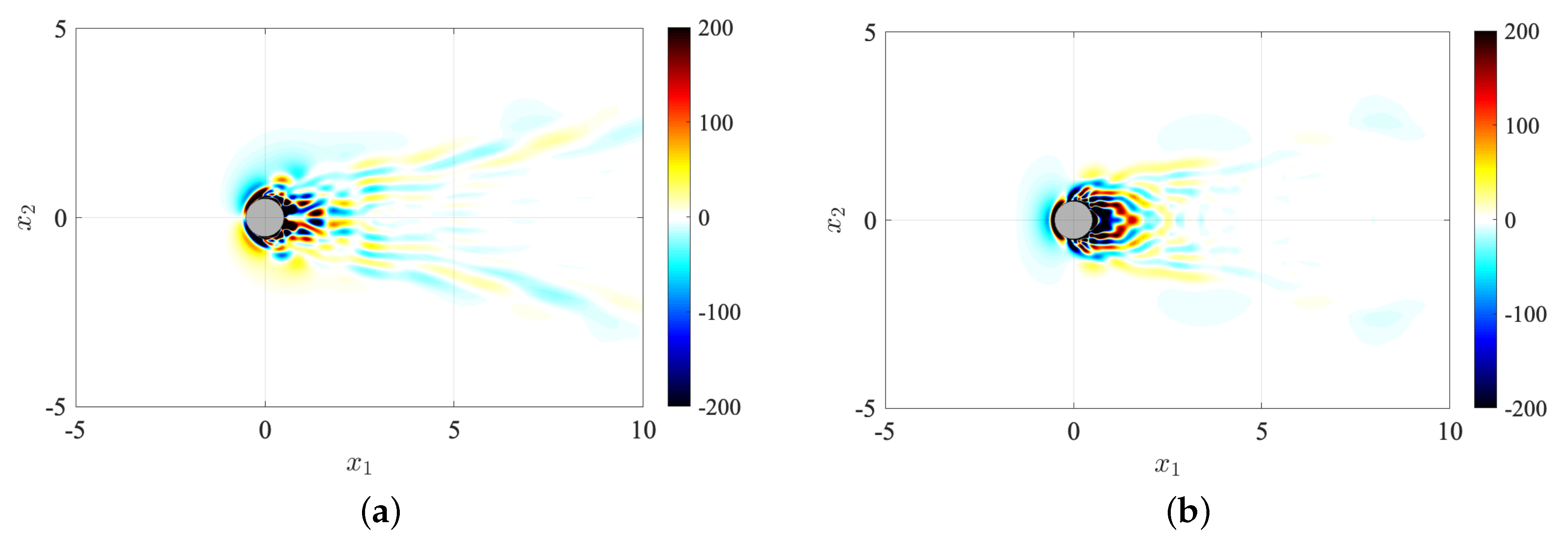
Figure 3a,b show the vorticity distribution before and after applying the MPC, respectively. The clockwise and counterclockwise vortices are filled by cold and warm colors, respectively. In the flow before applying the MPC (Figure 3a), the asymmetry of the vorticity peculiar to vortex shedding can be seen. In contrast, in the flow after applying the MPC (Figure 3b), the asymmetry of the vorticity is mitigated. This means that the vortex shedding is suppressed. It is found that two symmetric vortices in the flow with the MPC are remarkably larger than the ones arising at $Re\sim 10$. Although the pair of large vortices generally breaks soon without control, they can be maintained by the MPC.

We quantitatively evaluate the flow asymmetry with the use of the asymmetry function ${\mathsf{\Phi }}_{\mathrm{Asym}}\left(\tau \right)$. The time histories of ${\mathsf{\Phi }}_{\mathrm{Asym}}\left(\tau \right)$ without control and with the MPC are shown in Figure 4. Without control, the asymmetry function oscillates around ${\mathsf{\Phi }}_{\mathrm{Asym}}\left(\tau \right)=19$. In contrast, with the MPC, it can be seen that ${\mathsf{\Phi }}_{\mathrm{Asym}}\left(\tau \right)$ gradually decreases after the temporal increase and takes almost zero at the time $t=25$.

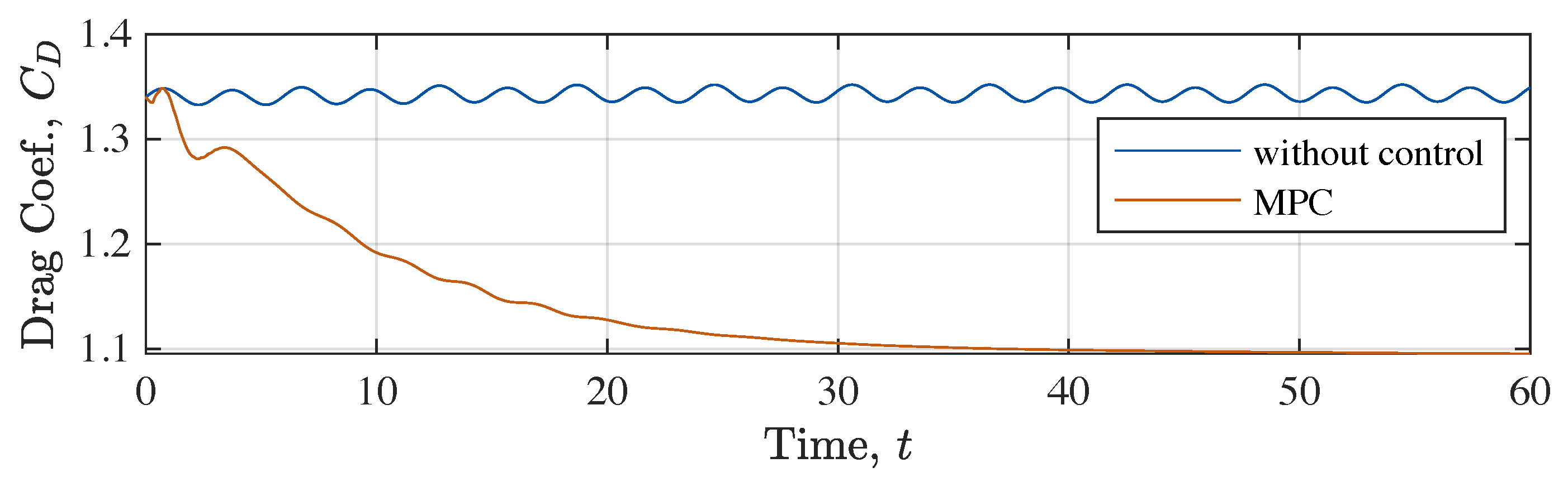
It is known that vortex shedding contributes to the increase in the drag of the cylinder. Figure 5 shows the time history of the drag coefficient without control and with the MPC. It is observed that the drag decreases by suppressing vortex shedding, and the range of the reduction is finally $18\%$. Comparing the Figure 4 and Figure 5, we can see that the drag coefficient continues to decrease after $t=25$ when the asymmetry function becomes almost zero. This difference in settling time is due to the expansion of the vortices. The pair of vortices continues to expand after $t=25$, when the flow becomes almost symmetric. This expansion intensifies the backward flow toward the cylinder. It is considered that the backward flow increases the pressure behind the cylinder, and therefore, the drag continues to decrease.

The time history of the jet speed, which is manipulated quantity, is shown in Figure 6. Although the jet speed fluctuates significantly on $0\le t\le 3$, the fluctuation gradually decreases. In order to evaluate the magnitude of the jet speed, we use the momentum coefficient defined by the following equation:

$$\begin{array}{c}\hfill C_{\mu }\left(t\right)=2U^2\left(t\right)d,\end{array}$$

(26)

where $d=|{\mathsf{\Gamma }}_{\mathrm{c},1}|=|{\mathsf{\Gamma }}_{\mathrm{c},2}|$ is the size of the jet holes. The momentum coefficient is the ratio of the momentum flux due to the free stream toward the cylinder to the one due to the two jets. The momentum coefficient is computed over the interval $0\le t\le 60$, and the maximum value $0.082$ was obtained at time $t=1.2$. This result suggests that the momentum flux due to the two jets is only $8.2\%$ of the one due to the free stream at most.

Computation of the control input in the MPC was performed on the workstation Mac Pro Late 2013 (CPU: 6-Core Intel Xeon E5 at 3.5 GHz, RAM: 32 GB) and the numerical computing environment MATLAB. The control input was computed 200 times on the overall interval $0\le t\le 60$, and it took 9 h and 36 min for the computation. On average, the computation time of the control input is about 3 min per control cycle. With this computation time, implementation of the MPC is limited to the extremely slow flow. The problem concerning online computation arises when applying MPC to general fluid flows as well as the flow around the cylinder. The MPC requires solving optimal control problems to compute the control input. The optimal control problems whose constraints include the Navier–Stokes equations has considerably high computational complexity. This obstacle must be removed to implement the MPC in actual fluid flows.

4. Design of Control Laws by Regression

We confirmed that it is difficult to implement MPC in actual flows in the previous section. However, it is possible to implement the MPC in the simulated virtual flow systems by taking much time on a computer. In this paper, control laws with low computational complexity are extracted from the data obtained in numerical simulations of controlled systems using the MPC.

Figure 7 schematically illustrates our proposed method for design of control laws. This design method is composed of the following two-step procedure:

• Store the time-series data of the optimal control input and the physical quantities obtained by applying MPC to the fluid flow in numerical simulations. These physical quantities are ones fed back to the new control law.
• Extract the function between the physical quantities and the optimal control input from the acquired data by using the regression analysis. This regression function is used as the control law.

Since the control law obtained by the proposed method estimates the optimal control input, it imitates conventional MPC. Moreover, the control law can be written in the explicit form and does not require solving optimal control problems online. Therefore, online computational complexity of the control law is quite small.

Table 2. Control laws designed by the proposed method.

Control Law	Quantities to be Fed Back	Regression Method
state-feedback law (SF-1)	velocity and in the whole region	ridge regression
state-feedback law (SF-2)	velocity and pressure in the whole region	ridge regression
output-feedback law (OF-1)	pressure on the surface	ridge regression
output-feedback law (OF-2)	pressure on the surface	Gaussian process regression

summarizes the control laws designed in this paper. We design two state-feedback control laws and two output-feedback control laws for flow around a cylinder. The spatially distributed velocity vector is fed back in the state-feedback control law (SF-1), and the velocity vector and the pressure are fed back in the state-feedback control law (SF-2). In the output-feedback control laws (OF-1) and (OF-2), the pressure on the cylinder surface is fed back. Since MPC originally feeds back state variables, it is reasonable to approximate the MPC as a state-feedback control law. However, it is practically difficult to measure the velocity distribution which is the state variable of the flow. Since the surface pressure can be measured relatively easily, the output-feedback control laws are easier to implement.

There is no guarantee that the optimal control input in MPC can be calculated from the surface pressure, which is not the state variable. However, it might be possible to calculate the optimal control input from the surface pressure because the optimal control input is determined implicitly, and what physical quantities are actually sensitive to the optimal control input is not known. We explore this possibility by extracting static output-feedback control laws.

We use ridge regression, which is a linear regression method, for extracting the two state-feedback control laws (SF-1) and (SF-2) and the output-feedback control law (OF-1). It is expected that a high-performance regression method is needed in order to estimate the optimal control input from the surface pressure. For extracting the output-feedback control law (OF-2), we use Gaussian process regression to obtain a nonlinear regression function. Since the control law extracted by Gaussian process regression is nonlinear, we expect that it performs better than the one extracted by linear regression.

First, in this section, we explain the details of the method to acquire training sets for the regression. Next, we explain the regression methods used in this paper.

4.1. Method to Produce Training Data

Solving optimal control problems for full-order fluid models requires quite high computation time. Since dimensions of the state variables are high in the optimal control problems, it is difficult to apply methods of placing training data points densely in the space of the state variable as in [23]. Against this background, we acquire time-series of the cylinder flow under MPC as training data, in the expectation that an attractor of the flow under the MPC are restricted to a low-dimensional space. If this expectation is true, an optimal control law of the MPC that are valid in the attractor could be extracted from a smaller number of elements in training data than the dimension of the state variable.

Figure 8 shows the method to produce the training data. This method includes two heuristic techniques to enhance generalization performance of the resulting control laws: use of different initial velocity distributions and addition of excitation noise. The cylinder flow without control changes periodically due to vortex shedding. We use the several flow fields in different phases as the initial conditions so that vortex shedding can be suppressed whenever the control starts. We acquire a time-series of the optimal control input and the physical quantities obtained by applying the MPC to each the initial flow field for training data. As excitation noise, the white Gaussian noise with mean zero is added to the optimal control input when applying the MPC. The reason for adding noise is to acquire the data not only on the attractor of the flow controlled by the MPC but also in its surroundings. This procedure is very similar to adding excitation noise in the identification of closed-loop systems. Although this paper does not provide the details, we have confirmed that control laws obtained using these heuristic techniques perform better than the ones obtained without using them.

We use an iterative procedure to determine the number of time-series datasets in training data. This procedure determines the number of time-series datasets based on the actual performance when the control law is applied to the baseline flow. We focus on the asymmetry function as the performance of the control law. A time-series with respect to the closed-loop system is added to the training data repeatedly and evaluate the change in the performance of the resulting control law due to the addition. We stop adding a time-series when this change in the performance becomes small because the performance of the resulting control law is not expected to be improved greatly by adding more time-series datasets to training data.

4.2. Regression Analysis Method

In regression analysis, the unknown relationship between an independent variable and a dependent variable is extracted from the training data. In order to design the control laws, we regard the independent variable as the physical quantities to be fed back (i.e., the velocity and pressure distribution in the state-feedback control laws and the surface pressure in the output-feedback control laws) and the dependent variable as the optimal control input.

4.2.1. Ridge Regression

Ridge regression is a type of linear regression. We assume the following linear relationship between the independent variable $\mathbf{w}\in {\mathbb{R}}^{n_w}$ and the dependent variable $z\in \mathbb{R}$:

$$\begin{array}{c}\hfill z=G\mathbf{w}.\end{array}$$

(27)

The goal of the ridge regression is to estimate the linear gain $G\in {\mathbb{R}}^{1\times n_w}$ in (27) from the given training data. Let us denote the training set of $\mathbf{w}$ by $\left\{{\mathbf{w}}_1,{\mathbf{w}}_2,\dots ,{\mathbf{w}}_M\right\}$ and the training set of z by $\{z_1,z_2,\dots ,z_M\}$. In the ridge regression, the gain G is estimated so that it minimizes the following function:

$$\begin{array}{c}\hfill \frac{1}{M}\sum _{m=1}^M{\left(z_m-G{\mathbf{w}}_m\right)}^2+{\rho }_{\mathrm{r}}{\parallel G\parallel }_2^2,\end{array}$$

(28)

where ${\rho }_{\mathrm{r}}$ is the positive number called the regularization parameter. The first term of the error function (28) represents the fitting error of the linear regression model for the training data, and the second term is added in order to prevent overfitting. If we define matrices related to the training data by $W={[{\mathbf{w}}_1,{\mathbf{w}}_2,\dots ,{\mathbf{w}}_M]}^{\mathsf{T}}$ and $\mathbf{Z}={[z_1,z_2,\dots ,z_M]}^{\mathsf{T}}$, the gain that minimizes the error function (28) is given by the following equation [33]:

$$\begin{array}{c}\hfill \widehat{G}={\mathbf{Z}}^{\mathsf{T}}{(W{W}^{\mathsf{T}}+M{\rho }_{\mathrm{r}}{I}_M)}^{-1}W,\end{array}$$

(29)

where $I_M$ is the $M\times M$ identity matrix. The matrix $\widehat{G}$ given in (29) is the gain estimated in the ridge regression.

4.2.2. Gaussian Process Regression

Since Gaussian process regression is based on a kernel method, it is effective even if the linear regression cannot fit training data well. In the Gaussian process regression, the following stochastic regression model is assumed:

$$\begin{array}{c}\hfill z=g\left(\mathbf{w}\right)+{ϵ}_0,\end{array}$$

(30)

where ${ϵ}_0\in \mathbb{R}$ is white Gaussian noise of mean zero and variance ${\gamma }_0$. The function $g\left(w\right)$ is a stochastic process, and for any finite number of independent variables ${\mathbf{w}}_1,{\mathbf{w}}_2,\dots ,{\mathbf{w}}_{\tilde{M}}$, the joint probability distribution of $g\left({\mathbf{w}}_1\right),g\left({\mathbf{w}}_2\right),\dots ,g\left({\mathbf{w}}_{\tilde{M}}\right)$ is a multivariate Gaussian distribution. A stochastic process with such properties is called a Gaussian process [34].

In the Gaussian process regression, the dependent variable is estimated from the training data sets by a Bayesian approach. Let us denote the mean function of the prior probability distribution $g\left(\mathbf{w}\right)$ by $m\left(\mathbf{x}\right)$ and the covariance function $E\left[g\left(\mathbf{w}\right)g\left({\mathbf{w}}^{\prime }\right)\right]$ by $k(\mathbf{w},{\mathbf{w}}^{\prime })$. Then, the probability distribution of z given $\mathbf{w}$ and the training data sets W and $\mathbf{Z}$ becomes a Gaussian distribution as follows [34]:

$$\begin{array}{cc}\hfill & p\left(z\right|\mathbf{w},W,\mathbf{Z})=\mathcal{N}(\mu ,\sigma ),\hfill \end{array}$$

(31)

$$\begin{array}{cc}\hfill & \mu \left(\mathbf{w}\right)={\mathbf{k}}^{\mathsf{T}}\left(\mathbf{w}\right){(K+{\gamma }_0^2{I}_M)}^{-1}(\mathbf{Z}-\mathbf{m}\left(\mathbf{w}\right)),\hfill \end{array}$$

(32)

$$\begin{array}{cc}\hfill & \sigma \left(\mathbf{w}\right)=k(\mathbf{w},\mathbf{w})-{\mathbf{k}}^{\mathsf{T}}\left(\mathbf{w}\right){(K+{\gamma }_0^2{I}_M)}^{-1}\mathbf{k}\left(\mathbf{w}\right),\hfill \end{array}$$

(33)

where $\mathcal{N}(\mu ,\sigma )$ is a Gaussian distribution with mean $\mu$ and standard deviation $\sigma$, and

$$\begin{array}{cc}\hfill \mathbf{k}\left(\mathbf{w}\right)& ={\left[k(\mathbf{w},{\mathbf{w}}_1),k(\mathbf{w},{\mathbf{w}}_2),\cdots ,k(\mathbf{w},{\mathbf{w}}_M)\right]}^{\mathsf{T}},\hfill \end{array}$$

(34)

$$\begin{array}{cc}\hfill K& =\left[\begin{array}{ccc}k({\mathbf{w}}_1,{\mathbf{w}}_1)& \cdots & k({\mathbf{w}}_1,{\mathbf{w}}_M)\\ ⋮& & ⋮\\ k({\mathbf{w}}_M,{\mathbf{w}}_1)& \cdots & k({\mathbf{w}}_M,{\mathbf{w}}_M)\end{array}\right],\hfill \end{array}$$

(35)

$$\begin{array}{cc}\hfill \mathbf{m}\left(\mathbf{w}\right)& ={\left[m\left({\mathbf{w}}_1\right),m\left({\mathbf{w}}_2\right),\cdots ,m\left({\mathbf{w}}_M\right)\right]}^{\mathsf{T}}.\hfill \end{array}$$

(36)

The mean function $\mu \left(\mathbf{w}\right)$ actually corresponds to the mean of the function $z\left(\mathbf{w}\right)$ given the training set. In the Gaussian process regression, the mean function $\mu \left(\mathbf{w}\right)$ is regarded as a function estimating the dependent variable from the independent variable.

The characteristics of the prior probability distribution $m\left(\mathbf{w}\right)$ and $k(\mathbf{w},{\mathbf{w}}^{\prime })$ determine basic properties of the estimating function $\mu \left(\mathbf{w}\right)$. In the regression problem we consider, $m\left(\mathbf{w}\right)$ and $k(\mathbf{w},{\mathbf{w}}^{\prime })$ are almost equal to the characteristics of the prior probability distribution of the optimal control law for the cylinder flow. However, we do not have any explicit knowledge about the optimal control law. Hence, we assume that $m\left(\mathbf{w}\right)$ constantly takes zero and $k(\mathbf{w},{\mathbf{w}}^{\prime })$ is the Gaussian kernel as follows:

$$\begin{array}{cc}\hfill m\left(\mathbf{w}\right)& =0,\hfill \end{array}$$

(37)

$$\begin{array}{cc}\hfill k(\mathbf{w},{\mathbf{w}}^{\prime })& ={\gamma }_1^{2}exp\left(-{\gamma }_2^2{\parallel \mathbf{w}-{\mathbf{w}}^{\prime }\parallel }^2\right),\hfill \end{array}$$

(38)

where ${\gamma }_1$ and ${\gamma }_2$ are the hyperparameters. According to the assumption of the Gaussian kernel (38), the closer the distance between two points $\mathbf{w}$ and ${\mathbf{w}}^{\prime }$, the stronger the correlation between the values on the two points $g\left(\mathbf{w}\right)$ and $g\left({\mathbf{w}}^{\prime }\right)$. The assumptions (37) and (38) are commonly used in the references about the Gaussian process regression.

The noise variance in the regression model and the parameters in the Gaussian kernel are estimated by likelihood maximization. Let us denote the parameters to be estimated by $\gamma ={[{\gamma }_0,{\gamma }_1,{\gamma }_2]}^{\mathsf{T}}$, and then the logarithm of the likelihood $p\left(\mathbf{Z}\right|W,\gamma )$ is given by the following equation:

$$\begin{array}{c}\hfill logp\left(\mathbf{Z}\right|W,\gamma )=-\frac{1}{2}{\mathbf{Z}}^{\mathsf{T}}{K}_z^{-1}\mathbf{Z}-\frac{1}{2}log\left|K_z\right|-\frac{n}{2}log2\pi ,\end{array}$$

(39)

where $K_z=K+{\gamma }_0^2{I}_M$. Since the parameter $\gamma$ that maximizes the log-likelihood (39) cannot be solved analytically in general, the gradient method is used to estimate $\gamma$. We can compute the gradient of the log-likelihood by using the following equation [34].

$$\begin{array}{c}\hfill \frac{\partial }{\partial {\gamma }_i}logp\left(\mathbf{Z}\right|W,\gamma )=\frac{1}{2}{\mathbf{Z}}^{\mathsf{T}}{K}_z^{-1}\frac{\partial K_z}{\partial {\gamma }_i}{K}_z^{-1}\mathbf{Z}-\frac{1}{2}\mathrm{trace}\left(K_z^{-1}\frac{\partial K_z}{\partial {\gamma }_i}\right).\end{array}$$

(40)

5. Application of the Proposed Method to Flow around a Cylinder

We design the control laws for flow around a cylinder at $Re=100$ by the proposed method in this section. The obtained control laws are applied to the flow in the simulations, and the results are compared. In addition, we examine the performance of the control laws over $80\le Re\le 120$.

5.1. Control Laws

Table 3. Parameters for training data.

Parameter	Value
number of the training sets M	$16\times 200$
standard deviation of an addictive noise ${\sigma }_e$	0.5
Reynolds Number $Re$	100

shows the parameters related to the training data. The time-series data of length 200 is obtained by applying the MPC to the flow. The length of the time-series data corresponds to 60 in the scale of the continuous time. The iterative procedure in Section 4.1 makes us apply the MPC to 16 sets of initial velocity distribution. In total, we can use the training set with $16\times 200=3200$ pairs of the physical quantities to be fed back and the optimal control input. We confirm that the number of time-series in the training data is sufficient in Section 5.3. The standard deviation of the noise added to the closed-loop system is 0.5. Four control laws are extracted from the training set.

5.1.1. State-Feedback Control Law (SF-1)

The state-feedback control law (SF-1) is extracted with the ridge regression from the training data of the optimal control input and the discretized flow velocity in the whole domain. The regularization coefficient is set to ${\rho }_{\mathrm{r}}=3\times {10}^{-6}$. Based on the symmetry of the optimal control problem with respect to $x_2=0$, we add constraints to the gain in the regression process so that it is antisymmetric with respect to $x_2=0$ for $u_1$ and symmetric for $u_2$. Figure 9a,b respectively show the obtained linear gain for $u_1$ and $u_2$. The cold, warm, and white fills respectively illustrate the regions where the gain is negative, positive, and nearly zero. The control input is determined by multiplying the control gains shown in Figure 9a,b by $u_1$ and $u_2$, respectively. As shown in the figures, the magnitude of the gain is large near the cylinder, especially behind the cylinder. Considering that vortex shedding occurs behind the cylinder, such a distribution of the control gain is reasonable.

5.1.2. State-Feedback Control Law (SF-2)

The state-feedback control law (SF-2) is extracted with the ridge regression from the training data of the optimal control input and the discretized flow velocity and pressure in the whole domain. The regularization coefficient is set to ${\rho }_{\mathrm{r}}=3\times {10}^{-6}$. Figure 10a–c respectively show the obtained linear gain for $u_1$, $u_2$, and p.

The control input is determined by multiplying the control gains shown in Figure 10a–c by $u_1$, $u_2$ and p, respectively. The discretized pressure is quadratic of the discretized velocity because it is obtained by numerically solving the pressure equation ${\nabla }^{2}p=\nabla ·\nabla ·(\mathbf{u}\otimes \mathbf{u})$. Hence, including p in the independent variables of the regression problem is expected to endow the resulting state-feedback control law (SF-2) with a sort of nonlinearity with respect to the state variable $\mathbf{u}$ unlike the state-feedback control law (SF-1).

5.1.3. Output-Feedback Control Law (OF-1)

The output-feedback control law (OF-1) is extracted with the ridge regression from the training data of the optimal control input and the discretized surface pressure. The regularization coefficient is set to ${\rho }_{\mathrm{r}}=3\times {10}^{-6}$. In addition, the control gain is constrained to be antisymmetric with respect to $x_2=0$ for the same reason as when designing the state-feedback control law (SF-1). Figure 11 shows the obtained control gain distribution. The control input is determined by multiplying the gain shown in Figure 11 by the pressure on the cylinder surface. It can be seen that the sign of the control gain is reversed many times from the front $\theta =\pm {180}^{\circ }$ to the rear $\theta =0^{\circ }$ of the cylinder.

5.1.4. Output-Feedback Control Law (OF-2)

The output-feedback control law (OF-2) is extracted with the Gaussian process regression. We use the quasi-Newton method for optimizing the hyperparameter $\gamma$. In the quasi-Newton method, the update of the Hessian matrix is done by SR1 (Symmetric Rank One), and the update width of the solution is determined by the trust region method. The initial candidate of the optimal solution is set to $\gamma ={[3\times {10}^{-2},1,{10}^{-3}]}^{\mathsf{T}}$, and, as the result of the optimization, $\gamma ={[916,0.0554,0.0549]}^{\mathsf{T}}$ is obtained. In (OF-2), the control input can be computed by substituting the surface pressure into $\mathbf{w}$ of the equation (32) under this hyperparameter. Unlike the other three control laws, it is difficult to visualize the gain because the control law (OF-2) is complicated.

5.2. Results and Discussion

The four designed control laws are applied to flow around a cylinder at Reynolds number $Re=100$. At this time, it is assumed that the physical quantities in the whole domain are available for computing the control input as in Section 3. Figure 12a–d respectively show the vorticity distribution under the control laws (SF-1), (SF-2), (OF-1), and (OF-2). In Figure 12a,b, the asymmetric vortices almost disappear. This suggests that the vortex shedding is suppressed under the two state-feedback control laws. On the other hand, under the two output-feedback control laws, the vortex shedding is not completely suppressed although the asymmetry of the vorticity is weakened as shown in Figure 12c,d.

Figure 13a shows the time history of the asymmetry function under the four control laws and the MPC for comparison. The performance of the two state-feedback control laws is close to that of the MPC. Although the two output-feedback control laws (OF-1) and (OF-2) are not comparable to the state-feedback control laws, they achieve about $40\%$ reduction in the asymmetric function. The performance in terms of the drag coefficient shows the same tendency as shown in Figure 13b. The two state-feedback control laws achieve almost the same reduction as the MPC, whereas the reduction under the two output-feedback control laws is only about 10%. Since the symmetric vortices do not develop greatly for the two output-feedback control laws, the back flow to the rear of the cylinder do not grow strong, and the drag do not decrease much.

Figure 13c,d are the enlarged and overall views of the manipulation variable over time. The jet speed under the two state-feedback control laws is similar to the one under the MPC at least on $0\le t\le 30$. Similarly, the two output-feedback control laws cause the jet speed that is consistent with the one under the MPC on $0\le t\le 4$. However, the change in the jet speed does not converge, and the oscillation continues until the control ends.

The same workstation as in Section 3 was used to compute the control input. The control laws (SF-1), (SF-2), (OF-1), and (OF-2) required $6.1\times {10}^{-5}$ s, $6.2\times {10}^{-5}$ s, $2.8\times {10}^{-5}$ s, and $2.8\times {10}^{-3}$ s to compute the control input at each time step, respectively. The computation time of the control law (OF-2) is particularly longer because the computation of the Gaussian kernel $\mathbf{k}$ in the expression (32) is complicated.

Although the four newly designed control laws vary in the computation time as described above, they are more realistic to implement in actual controlled flow systems than the MPC, whose computation time is 180 s.

To summarize the above results, the state-feedback control laws (SF-1) and (SF-2) are able to imitate the MPC at least for the flow at $Re=100$, and the control input can be computed with low computational complexity. Although the output-feedback control laws (OF-1) and (OF-2) also have low computational complexity, their ability to suppress vortex shedding is inferior to that of the MPC. In order to consider the difference in performance between the four control laws, we examine the error in each control law.

The RMSPE (Root Mean Square Percentage Error) defined below is used to evaluate the error in each control law:

$$\begin{array}{c}\hfill \mathrm{RMSPE}=\sqrt{\frac{{\sum }_{m=1}^{L_{\mathrm{data}}}{({\widehat{z}}_m-z_m)}^2}{{\sum }_{m=1}^L{z}_m^2}},\end{array}$$

(41)

where $L_{\mathrm{data}}$ is the data length, $z_m$ is the true optimal control input, and ${\widehat{z}}_m$ is the optimal control input estimated by the control law. The RMSPE values of the control laws are examined for the training data and the test data. The training data is the data used for learning the control laws. As the test data, we use a time-series that is obtained by applying each the control law to the flow. Applying the control law causes the different state transitions as shown above. The time-series datasets of the true optimal control input are newly obtained by solving the optimal control problems along these state transitions over $0\le t\le 60$.

Table 4. Training and test errors of the four control laws.

	Control Law (SF-1)	Control Law (SF-2)	Control Law (OF-1)	Control Law (OF-1)
training error	7.8%	3.9%	31.9%	28.3%
test error	29.0%	15.4%	99.3%	98.2%

shows the errors in the four control laws for the training and test data. In all the control laws, the test error is larger than the training error. The state feedback control law (SF-2) estimates the optimal control input with the minimum error for each the training and test data of all the control laws. The estimation accuracy of the state-feedback control law (SF-2) is the second best after (SF-1). While the training errors of the output-feedback control laws (OF-1) and (OF-2) are about $30\%$, the test errors exceed $90\%$. This indicates that the output-feedback control laws hardly estimate the optimal control input when applying them to the flow. In fact, although the output-feedback control laws estimate well immediately after the control starts, their estimation accuracies gradually deteriorate. For this reason, it is considered that the output-feedback control laws cannot completely suppress the vortex shedding. It is also interesting that the training errors in the two output-feedback control laws extracted by linear regression and nonlinear Gaussian process regression are comparable. This fact might suggest that the limitation of estimating the optimal control input from the surface pressure.

5.3. Performance over the Number of Trajectories in the Training Data

We examine the performance of the control laws over the number of time-series in the training set to confirm whether 16 time-series are sufficient to extract the control laws that perform well. The training datasets composed of 1, 2, 4, 8, and 12 time-series were generated by thinning out some time-series from the training data with the 16 time-series. We extract the four control laws from each of the training datasets and apply them to flow around the cylinder at $Re=100$. Figure 14a–d show the asymmetry function under the control laws (SF-1), (SF-2), (OF-1), and (OF-2) over the number of trajectories in the training set, respectively.

It is observed that increasing the time-series improves the performance of the control laws with few exceptions. Furthermore, as the number of trajectories in the training set increases, the change in the asymmetry function due to this increase gradually decreases. Under the output-feedback control laws extracted from the dataset with the 8 or more time-series, the asymmetry functions behave the same as each other. In addition, there is no remarkable difference in the time histories of the asymmetry functions under the state-feedback control laws extracted from the 12 and 16 time-series. Hence, we infer from these results that further increase of the trajectory in the training set does not significantly improve the performance at least for flow around a cylinder at $Re=100$.

5.4. Performance over the Reynolds Number

While the four control laws were extracted from the data of only the flow at $Re=100$, it is interesting how robust these control laws are to the change in the Reynolds number. In this subsection, we examine the performance of the control laws for several Reynolds numbers different from 100.

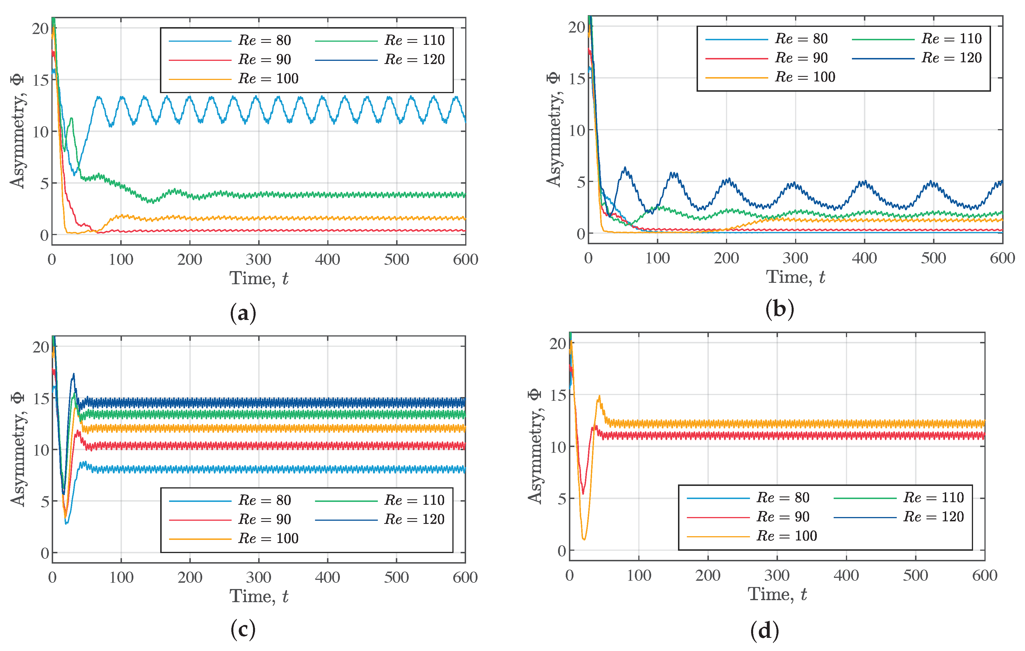
In numerical simulations, each of the control laws (SF-1), (SF-2), (OF-1), and (OF-2) is applied to the flows at $Re=80$, 90, 100, 110, and 120. Figure 15a–d show the asymmetry functions under the control laws (SF-1), (SF-2), (OF-1), and (OF-2), respectively. The results for $Re=80$, 90, 100, 110, and 120 are shown in different colors. The state-feedback control law (SF-2) remarkably reduces the asymmetry for all the Reynolds numbers. Similarly, the asymmetry function under the output-feedback control law (OF-1) is moderately weakened for any Reynolds number. Under the control laws (SF-2) and (OF-1), the higher the Reynolds number, the bigger the asymmetry function is in a steady-state. This relationship between the Reynolds number and the asymmetry might be attributed to flow instability. According to the stability analysis in [35], amplitude of perturbations of steady flows strengthens as the Reynolds number increases. In fact, we confirm that the asymmetry function under no control increases with increasing Reynolds number in simulations. Since the flow around a cylinder has such a characteristic, it is considered that the higher the Reynolds number of the flow than the one used for training data, the more difficult to suppress the vortex shedding.

The asymmetry function under the state-feedback control law (SF-1) is similar to the one under the control law (SF-2) for $Re=90$, 100, and 110. However, for $Re=120$, the control input diverges and the control of the vortex shedding fails. Likewise, the results under the output-feedback control laws (OF-1) and (OF-2) are nearly identical for $Re=90$ and 100. On the other hand, the control input under (OF-2) diverges for $Re=80$, 110, and 120.

Summarizing the above results, of the two state-feedback control laws, the control law (SF-2), which feeds back not only the flow velocity but also the pressure, is more robust to changes in the Reynolds number. In addition, the output-feedback control law extracted by linear regression has higher robustness than the one extracted by Gaussian process regression. Note that the four control laws are extracted from the data of the flow only at $Re=100$. The robustness of the control laws is expected to be improved by using data of flows at different Reynolds numbers. However, the above analysis reveals that control laws extracted from data for single Reynolds number can be robust to a slight change in the Reynolds number.

6. Conclusions

Reduction of online computation time for MPC is a challenging issue for implementation in actual fluid flow systems. In this paper, control of flow around a cylinder was presented as a benchmark problem, and computationally-inexpensive control laws were extracted from the data obtained by offline optimization.

The two state-feedback control laws extracted by ridge regression showed the same behavior as MPC and was able to suppress vortex shedding successfully at $Re=100$. It is surprising that these control laws perform like MPC because there is no guarantee that the control law of the MPC is linear for the velocity or pressure. In addition, the time for computing the control input was quite shorter than MPC, and it is realistic for implementation.

We also designed two of practical output-feedback control laws which observe the surface pressure. The two output-feedback control laws were extracted by linear regression and nonlinear regression, respectively. Both of the output-feedback control laws could not suppress vortex shedding completely while the flow asymmetry was slightly mitigated. The low performance of the output-feedback control laws seems to be attribute to the fact that the MPC is originally a state-feedback control law.

Output-feedback controllers that perform well might be designed by combining state-feedback controllers and state estimators. However, state estimators for fluid flows generally have high computational complexity, and therefore, some method to reduce the computational cost is needed for online implementation. We will propose a method to solve this problem in state estimators in our future study.

The four control laws were extracted from the data of the flow only at $Re=100$, but they are robust to some change in the Reynolds number. Especially, the controller that feeds back the distribution of the velocity and pressure remarkably improved the flow asymmetry over $80\le Re\le 120$. It seems that a sort of nonlinearity given to the control law by feedback of the pressure contributed to the robustness. The output-feedback control law extracted by nonlinear Gaussian process regression has showed the lowest robustness. This fact indicates that nonlinear regression does not necessarily provide high robustness of control laws. However, data for different Reynolds numbers is expected to enhance robustness of the resulting control laws, especially when using nonlinear regression that fits the data well.

References

- Post, M.L.; Corke, T.C. Separation control on high angle of attack airfoil using plasma actuators. AIAA J. 2004, 42, 2177–2184. [Google Scholar] [CrossRef]
- Amitay, M.; Smith, D.R.; Kibens, V.; Parekh, D.E.; Glezer, A. Aerodynamic flow control over an unconventional airfoil using synthetic jet actuators. AIAA J. 2001, 39, 361–370. [Google Scholar] [CrossRef]
- Choi, K.S.; Jukes, T.; Whalley, R. Turbulent boundary-layer control with plasma actuators. Philos. Trans. R. Soc. A Math. Phys. Eng. Sci. 2011, 369, 1443–1458. [Google Scholar] [CrossRef] [PubMed]
- Patel, M.P.; Sowle, Z.H.; Corke, T.C.; He, C. Autonomous sensing and control of wing stall using a smart plasma slat. J. Aircr. 2007, 44, 516–527. [Google Scholar] [CrossRef]
- Pinier, J.T.; Ausseur, J.M.; Glauser, M.N.; Higuchi, H. Proportional closed-loop feedback control of flow separation. AIAA J. 2007, 45, 181–190. [Google Scholar] [CrossRef]
- Post, M.L.; Corke, T.C. Separation control using plasma actuators: Dynamic stall vortex control on oscillating airfoil. AIAA J. 2006, 44, 3125–3135. [Google Scholar] [CrossRef]
- Poggie, J.; Tilmann, C.P.; Flick, P.M.; Silkey, J.S.; Osbourne, B.A.; Ervin, G.; Maric, D.; Mangalam, S.; Mangalam, A. Closed-loop stall control system. J. Aircr. 2010, 47, 1747–1755. [Google Scholar] [CrossRef]
- Segawa, T.; Suzuki, D.; Fujino, T.; Jukes, T.; Matsunuma, T. Feedback control of flow separation using plasma actuator and FBG sensor. Int. J. Aerosp. Eng. 2016, 2016, 8648919. [Google Scholar] [CrossRef] [Green Version]
- Pastoor, M.; Henning, L.; Noack, B.R.; King, R.; Tadmor, G. Feedback shear layer control for bluff body drag reduction. J. Fluid Mech. 2008, 608, 161–196. [Google Scholar] [CrossRef] [Green Version]
- Becker, R.; King, R.; Petz, R.; Nitsche, W. Adaptive closed-loop separation control on a high-lift configuration using extremum seeking. AIAA J. 2007, 45, 1382–1392. [Google Scholar] [CrossRef]
- Benard, N.; Moreau, E.; Griffin, J.; Cattafesta, L.N. Slope seeking for autonomous lift improvement by plasma surface discharge. Exp. Fluids 2010, 48, 791–808. [Google Scholar] [CrossRef]
- Wu, Z.; Wong, C.W.; Wang, L.; Lu, Z.; Zhu, Y.; Zhou, Y. A rapidly settled closed-loop control for airfoil aerodynamics based on plasma actuation. Exp. Fluids 2015, 56, 1–15. [Google Scholar] [CrossRef]
- Choi, H.; Moin, P.; Kim, J. Active turbulence control for drag reduction in wall-bounded flows. J. Fluid Mech. 1994, 262, 75–110. [Google Scholar] [CrossRef]
- Lee, K.H.; Cortelezzi, L.; Kim, J.; Speyer, J. Application of reduced-order controller to turbulent flows for drag reduction. Phys. Fluids 2001, 13, 1321–1330. [Google Scholar] [CrossRef] [Green Version]
- Bagheri, S.; Brandt, L.; Henningson, D.S. Input–output analysis, model reduction and control of the flat-plate boundary layer. J. Fluid Mech. 2009, 620, 263–298. [Google Scholar] [CrossRef] [Green Version]
- Semeraro, O.; Bagheri, S.; Brandt, L.; Henningson, D.S. Feedback control of three-dimensional optimal disturbances using reduced-order models. J. Fluid Mech. 2011, 677, 63–102. [Google Scholar] [CrossRef] [Green Version]
- Huang, S.C.; Kim, J. Control and system identification of a separated flow. Phys. Fluids 2008, 20, 101509. [Google Scholar] [CrossRef] [Green Version]
- Bewley, T.R.; Moin, P.; Temam, R. DNS-based predictive control of turbulence: An optimal benchmark for feedback algorithms. J. Fluid Mech. 2001, 447, 179–225. [Google Scholar] [CrossRef] [Green Version]
- Yamamoto, A.; Hasegawa, Y.; Kasagi, N. Optimal control of dissimilar heat and momentum transfer in a fully developed turbulent channel flow. J. Fluid Mech. 2013, 733, 189–220. [Google Scholar] [CrossRef]
- Protas, B.; Styczek, A. Optimal rotary control of the cylinder wake in the laminar regime. Phys. Fluids 2002, 14, 2073–2087. [Google Scholar] [CrossRef]
- Flinois, T.L.; Colonius, T. Optimal control of circular cylinder wakes using long control horizons. Phys. Fluids 2015, 27, 087105. [Google Scholar] [CrossRef] [Green Version]
- Sasaki, Y.; Tsubakino, D. Model predictive control of a separated flow around a circular cylinder at a low Reynolds number. SICE J. Control Meas. Syst. Integr. 2018, 11, 154–159. [Google Scholar] [CrossRef] [Green Version]
- Mathelin, L.; Pastur, L.; Le Maître, O. A compressed-sensing approach for closed-loop optimal control of nonlinear systems. Theor. Comput. Fluid Dyn. 2012, 26, 319–337. [Google Scholar] [CrossRef]
- Arian, E.; Fahl, M.; Sachs, E.W. Trust-Region Proper Orthogonal Decomposition for Flow Control; Technical Report; Institute for Computer Applications in Science and Engineering: Hampton, VA, USA, 2000.
- Ravindran, S. Reduced-order adaptive controllers for fluid flows using POD. J. Sci. Comput. 2000, 15, 457–478. [Google Scholar] [CrossRef]
- Kaiser, E.; Noack, B.R.; Cordier, L.; Spohn, A.; Segond, M.; Abel, M.; Daviller, G.; Östh, J.; Krajnović, S.; Niven, R.K. Cluster-based reduced-order modelling of a mixing layer. J. Fluid Mech. 2014, 754, 365–414. [Google Scholar] [CrossRef] [Green Version]
- Sasaki, Y.; Tsubakino, D. Explicit model predictive control with Gaussian process regression for flows around a cylinder. IFAC PapersOnLine 2018, 51, 38–43. [Google Scholar] [CrossRef]
- Marquet, O.; Sipp, D.; Jacquin, L. Sensitivity analysis and passive control of cylinder flow. J. Fluid Mech. 2008, 615, 221–252. [Google Scholar] [CrossRef] [Green Version]
- Guéniat, F.; Mathelin, L.; Hussaini, M.Y. A statistical learning strategy for closed-loop control of fluid flows. Theor. Comput. Fluid Dyn. 2016, 30, 497–510. [Google Scholar] [CrossRef] [Green Version]
- Min, C.; Choi, H. Suboptimal feedback control of vortex shedding at low Reynolds numbers. J. Fluid Mech. 1999, 401, 123–156. [Google Scholar] [CrossRef] [Green Version]
- Nocedal, J.; Wright, S. Numerical Optimization, 2nd ed.; Springer Science: New York, NY, USA, 2006. [Google Scholar]
- Spalart, P.R.; Moser, R.D.; Rogers, M.M. Spectral methods for the Navier–Stokes equations with one infinite and two periodic directions. J. Comput. Phys. 1991, 96, 297–324. [Google Scholar] [CrossRef]
- Bishop, C.M. Pattern Recognition and Machine Learning; Springer: New York, NY, USA, 2006. [Google Scholar]
- Rasmussen, C.E.; Williams, K.I. Gaussian Processes for Machine Learning; The MIT Press: Cambridge, MA, USA, 2006. [Google Scholar]
- Provansal, M.; Mathis, C.; Boyer, L. Bénard-von Kármán instability: Transient and forced regimes. J. Fluid Mech. 1987, 182, 1–22. [Google Scholar] [CrossRef]
Figure 1.
Control input in MPC. The blue histogram shows control input in MPC, and the three gray histograms show optimal control inputs obtained at , , and .
Figure 2.
Geometry of flow around a cylinder. (a): an overall view, (b): an enlarged view.
Figure 3.
Contours of the vorticity of the flows (a) without control and (b) with MPC).
Figure 4.
History of the asymmetric function. (Blue line: Without control, Red line: With MPC).
Figure 5.
History of the drag coefficient. (Blue line: Without control, Red line: With MPC).
Figure 6.
History of the jet speed.
Figure 7.
Outline of the proposed method.
Figure 8.
The method to produce training data sets.
Figure 9.
Gain of the control law (SF-1) for (a) and (b) .
Figure 10.
Gain of the control law (SF-2) for (a) , (b) , and (c) p.
Figure 11.
Gain for the pressure on the surface. The angle takes zero at the right edge of the cylinder.
Figure 12.
Contours of the vorticity of the flows under (a) the control laws (SF-1), (b) (SF-2), (c) (OF-1), and (d) (OF-2).
Figure 13.
Plots of (a) the asymmetric function, (b) the drag coefficient, (c), (d) the control input. The cyan, yellow, red, green, and dashed lines respectively show the results under the control laws (SF-1), (SF-2), (OF-1), (OF-2), and the MPC.
Figure 14.
History of the asymmetry function under the control laws over the number of the trajectories of the training datasets. (a): the control law (SF-1), (b): the control law (SF-2), (c): the control law (OF-1), (d): the control law (OF-2).
Figure 15.
Histories of the asymmetry functions under the control laws for , 90, 100, 110, and 120. (a): the control law (SF-1), (b): the control law (SF-2), (c): the control law (OF-1), (d): the control law (OF-2). Some lines in (a) and (d) are hardly seen because the control input diverges immediately after the control starts.