New Criteria to Characterize the Waste Heat Recovery

Abstract

Waste heat recovery is an actual goal. The best way to valorize waste heat is to use it directly with the appropriate level of temperature. If the temperature level is insufficient, many reverse machine configurations are available in order to obtain the appropriate conditions (the most known are heat pumps and heat transformers). Finally, the remaining unused heat could be converted to any noble form of energy (mechanical, electrical essentially). We propose here to examine, with a new point of view, the thermomechanical conversion limit of waste heat. This limit corresponds to adiabatic conversion for an endo-reversible Carnot engine, with a perfect thermal contact at the atmospheric sink (supposed infinite). The Carnot–Chambadal model version is applied to latent and sensible heat recovery cases. The results associated with these two cases differ fundamentally. Comments are provided on the two studied cases, and new criteria to characterize the corresponding waste heat recovery are proposed.

1. Introduction

Waste heat recovery is essential for increasing energy efficiency in different industry sectors. Increasing energy costs and environmental concerns provide strong motivation for implementing more and newer methods and technologies for waste heat recovery.

Recent papers [1,2,3,4] prove that this topic is a well-studied one by the analysis of thermodynamic models for the simulation and optimization of power systems [1,2], as well as energy and exergy analysis of waste heat recovery systems [3,4]. For instance, an assessment with the citation indexing service Web of Science, that provides a comprehensive citation search through multiple databases, gives for “waste heat” a total of 23,717 references within its core collection over the period 1950–2017, of which 313 are highly cited. Over the last five years, an increase of 25% of the publication is observed to reach a high-level amount of 2753 in 2016. The main contributive organizations on this topic are the United States Department of Energy (DOE) with 625 references, the Chinese Academy of Science with 345 one and the French national scientific research center CNRS with 287. Among all these publications, 7239 are related to energy fuels, 3700 to chemical engineering, 3444 to thermodynamics, 3274 to environmental sciences and 2865 to mechanical engineering. The proposed analysis clearly concerns thermodynamics and mechanical engineering.

The use of conventional waste heat recovery technologies depends on the temperature of the waste heat stream, the composition of the waste heat stream and the available heat transfer area. They have been classified into active and passive technologies, with subcategories depending on the application to provide heating, cooling or electricity [5].

The methods commonly involved are (i) direct utilizing: heat delivery to district heating or cooling or preheating; (ii) power utilizing: electricity generation using generator; and (iii) cascade utilization: combining heating, cooling and power [6].

Generally, heat recovery technologies can be grouped into [7]:

-

Technologies that recover heat from a primary flow and make it available as the heat of lower or similar quality in a secondary flow, for which typical examples are the recuperators, regenerators and different type of heat exchangers;

-

Technologies that recover heat from a primary flow and upgrade this to a higher temperature useful heat using another heat source as input, and;

-

Technologies that recover and convert heat from a primary flow to electricity. Typical examples are the conventional Steam Rankine Cycle and the Organic Rankine Cycle. Other potential systems at different stages of research, development and application include the Organic Flash Cycle, the Kalina Cycle, the Trilateral Flash Cycle and the Supercritical CO₂ Brayton Cycle.

Typical waste heat recovery devices include recuperators, furnace regenerators, recuperative and regenerative burners, passive air preheaters, heat exchangers (shell and tube, finned tube, flat plate, heat pipes) or economizers, rotary regenerator or heat wheel, preheating of load, waste heat boilers and heat pumps.

Among the novel and promising technologies for waste heat recovery, thermoelectric systems have been well considered [8,9,10,11,12,13], while others, such as piezoelectric devices [14] are not much studied and developed. Organic Rankine Cycle (ORC) has been highly discussed for many years with subcritical and transcritical configurations. The main goals of waste heat recovery technology are to choose optimal operating conditions and the working fluid. One recent example is relative to geothermal power plants [15,16,17].

In thermomechanical systems, the energy from waste heat can be recovered as sensible or latent heat. In the classical heat exchangers used, for example in cascade heat recovery by thermal engines (internal combustion engines, gas turbine engines), the heat transfer from one fluid to the other is done by sensible heat causing a change in temperature for each fluid. In the phase change heat exchangers (in Organic Rankine Cycle technology, heat pumps), the corresponding energy transfer is done by latent heat that causes a change of state with no change in temperature for pure substances.

Generally, the optimization of the waste heat valorization in thermomechanical systems has the recovered energy or the mechanical power output as objective function or criteria. In addition to them, energy efficiency or exergy efficiency can also be considered. Many papers consider exergy and economic analysis for simple as well as for complex systems [4,18,19,20]. Unfortunately, energy efficiency and exergy efficiency are not always relevant, particularly for the case of waste heat recovery as sensible heat. This issue challenged us to find more appropriate criteria that better reflect the efficiency of waste heat recovery technologies.

Thus, this paper focuses on the evaluation of the potential for waste heat recovery with a highlight on process efficiency limit from the simplest configuration of ORC with latent or sensible waste heat. The valorizing limits (exergetic ones) are exemplified, optimization of the mechanical power is achieved and its consequences are analyzed with consideration of various efficiencies.

The paper topic is mainly concerned by fundamental aspects and methodology than by aspects developed regarding process sites, even if these developments become more and more explored [2,3,21,22,23,24].

For these reasons, the paper presents two different models that can be used: firstly, the latent heat valorization one, and secondly, the sensible heat valorization, both considering the finite source and sink. The obtained results are discussed starting from the presentation of the optimum mechanical recuperation for Chambadal’s model and the exergetic efficiency when considering sensible heat.

Our proposal of two new criteria called “recovery ratio”, refers either to maximum recoverable energy on heat form (independently of process), τ_ES, or to maximum recoverable exergy, τ_Ex. They characterize the energetic (exergetic) performance of a valorizing process and can be useful to wisely choose the technical solutions for an efficient waste heat recovery by different technologies.

2. The Models of the Thermomechanical Heat Recovery

The objective of this section is to report on two models useful to characterize the mechanical valorization of heat. The first model is relative to the latent heat valorization. The second one is relative to sensible heat valorization. The two models are developed with the same hypothesis:

• A steady state is considered and;
• Thermal losses are neglected.

Knowing the available waste heat, the maximum mechanical power is sought. Nondimensional valorization criteria are presented and compared.

2.1. Latent Heat Valorization Model

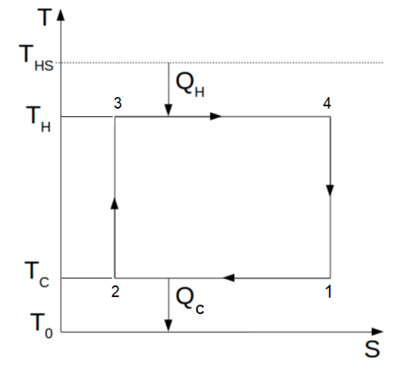
The hot source is in the form of latent heat rate $\dot{Q_0}$ available at temperature T_HS. The waste heat valorization is studied with respect to the ambient temperature T₀. Figure 1 is a representation in temperature—an entropy diagram of the latent heat valorization by means of an endo-reversible Carnot engine. Thus, a third hypothesis is added: the studied case is an endo-reversible one.

Indeed, the Carnot cycle represented in the textbook remains generally totally reversible. The basic heat engine model refers to equilibrium thermodynamics in order to obtain the maximum limit of energy efficiency (first law efficiency) between two reservoirs at constant temperature (thermostats) respectively T_HS at the heat source, T_CS = T₀ at the cold sink.

However, an engine functioning in these conditions would produce no power. So, a more realistic model is to consider a difference of temperature between the reservoirs (source and sink) and the Carnot cycle or engine: this is the endo-reversible model examined hereafter, completed and particularized to latent heat recovery.

2.1.1. Carnot Endo-Reversible Model

Results concerning the Carnot engine analytical approach are available in the literature [25,26]. The reported model is precisely an adaptation of the Curzon–Ahlborn one applied to the studied case.

The heat rates at source and sink are supposed obeying a linear heat transfer law such that:

$${\dot{Q}}_H = K_H\left(T_{HS}–T_H\right),$$

(1)

$${\dot{Q}}_C = K_C\left(T_C–T_0\right),$$

(2)

where K_H and K_C are the heat transfer conductances at the hot side and cold side of the system, respectively; T_H is the cycled fluid temperature at the hot side and T_C is the cycled fluid temperature at the cold side.

In a first attempt K_H, K_C, T_HS and T₀ are constant parameters. The mechanical power delivered by the engine results from the energy balance:

$$\dot{W} = {\dot{Q}}_H-{\dot{Q}}_C,$$

(3)

where $\dot{Q_H}$ is the thermal heat rate exchanged at the hot source, $\dot{Q_C}$ is the thermal rate exchanged at the cold sink and $\dot{W}$ is the mechanical power output.

There are two control variables T_H and T_C but linked by the entropic balance at the converter (one degree of freedom):

$$\frac{{\dot{Q}}_H}{T_H} = \frac{{\dot{Q}}_C}{T_C}.$$

(4)

The resolution by variational calculation assumes the following Lagrange function:

$$L\left(T_H,T_C \right) = \dot{W}+\lambda \left(\frac{{\dot{Q}}_H}{T_H}-\frac{{\dot{Q}}_C}{T_C}\right).$$

(5)

Hence, the necessary condition of the optimum power $Ma{x}_1(\dot{W})$ is achieved for:

$$T_H{}^{*} = \sqrt{T_{HS}}·F_K,$$

(6)

$$T_C{}^{*} = \sqrt{T_0}·F_K,$$

(7)

with

$$F_K = \frac{K_H\sqrt{T_{HS}}+K_C\sqrt{T_0}}{K_H+K_C}.$$

(8)

The maximum power is deduced as:

$$Ma{x}_1\dot{W} = \frac{K_H{K}_C}{K_H+K_C}{\left(\sqrt{T_{HS}}-\sqrt{T_0}\right)}^2,$$

(9)

and the efficiency according to the first law associated to this maximum:

$${\eta }_I\left(Ma{x}_1\dot{W}\right) = 1-\sqrt{\frac{T_0}{T_{HS}}}.$$

(10)

This efficiency corresponds to the one proposed by Curzon and Ahlborn [6], but it can be noticed that a second sequential optimization is possible [10] when considering the finite physical dimension constraint relative to the heat transfer conductances:

$$K_H+K_C = K_T.$$

(11)

By using the same methodology as in the first optimization, it is found that $Ma{x}_2(\dot{W})$ corresponds to the equipartition of the heat transfer conductances for the endo-reversible engine:

$$K_H{}^{*} = K_C{}^{*}= \frac{K_T}{2},$$

(12)

where K_T is the total heat transfer conductance to be allocated.

By using the expression of the two heat transfer conductances from Equation (12) in Equation (9), ${Max}_2(\dot{W})$ results as:

$$Ma{x}_2\dot{W} = \frac{K_T}{4}{\left(\sqrt{T_{HS}}-\sqrt{T_0}\right)}^2.$$

(13)

The efficiency at maximum power expression remains unchanged, but this solution corresponds to an optimal value of ${\dot{Q}}_H$:

$${\dot{Q}}_H\left(Ma{x}_2\dot{W}\right) = \frac{K_T}{4}\sqrt{T_{HS}}\left(\sqrt{T_{HS}}-\sqrt{T_0}\right).$$

(14)

2.1.2. Case with Latent Heat Rate Imposed by the Source

In the case of latent heat rate recovery, the available latent heat rate at the source is a constraint ${\dot{Q}}_0$. When replaced in Equation (1), this constraint determines T_H:

$$T_H = T_{HS}-\frac{{\dot{Q}}_0}{K_H}.$$

(15)

By using Equation (15) in the entropy balance expression (Equation (4)), one gets:

$$K_C\left(1-\frac{T_0}{T_C}\right) = \frac{{\dot{Q}}_0}{T_{HS}-\frac{{\dot{Q}}_0}{K_H}}.$$

(16)

After some calculations, the following expression for the temperature T_H is deduced from Equation (16):

$$T_C = T_0\frac{T_{HS}-\frac{{\dot{Q}}_0}{K_H}}{T_{HS}-{\dot{Q}}_0\left(\frac{1}{K_C}+\frac{1}{K_H}\right)}.$$

(17)

The power output of the engine depending on the heat rate imposed by the source results from Equation (3) when Equations (17) and (2) are considered:

$$\dot{W} = {\dot{Q}}_0\left[1-\frac{T_0}{T_{HS}-{\dot{Q}}_0\left(\frac{1}{K_C}+\frac{1}{K_H}\right)}\right].$$

(18)

It follows that $Ma{x}_1(\dot{W})$ corresponds here to the minimum of the sum $\left(\frac{1}{K_C}+\frac{1}{K_H}\right)$, associated to the finite dimension constraint (Equation (11)). It corresponds again to the equipartition of the heat transfer conductances (Equation (12)) for the endo-reversible engine, and its expression is:

$$Ma{x}_1\dot{W} = {\dot{Q}}_0\left[1-\frac{T_0}{T_{HS}-\frac{4·{\dot{Q}}_0}{K_T}}\right].$$

(19)

This solution is physically acceptable only if:

$${\dot{Q}}_0\le \frac{K_T}{4}\left(T_{HS}-T_0\right).$$

(20)

Otherwise, it can be seen on Equation (19) that an optimal value of ${\dot{Q}}_0$ exists with the given parameters T_HS, T₀ and K_T. It is easy to verify that this optimal value of $\dot{Q_0}$ is exactly the one given by Equation (14), as expected.

Moreover, $Ma{x}_1(\dot{W})$ constrained by the value $\dot{Q_0}$, leads to the associated efficiency according to first law:

$${\eta }_I\left(Ma{x}_1\dot{W}\right) = 1-\frac{T_0}{T_{HS}-\frac{4·{\dot{Q}}_0}{K_T}}.$$

(21)

The higher K_T is, the closer this efficiency is to Carnot’s efficiency one.

This efficiency is a decreasing function of ${\dot{Q}}_0$ in the range of permitted value for this variable (Equation (20)), and an increasing function of T_HS. Equation (21) confirms here that first law efficiency depends on extensities ${\dot{Q}}_0$, K_T as well as intensities T_HS; however, extensities are related by the quotient ${\dot{Q}}_0$/K_T that possesses an intensity dimension.

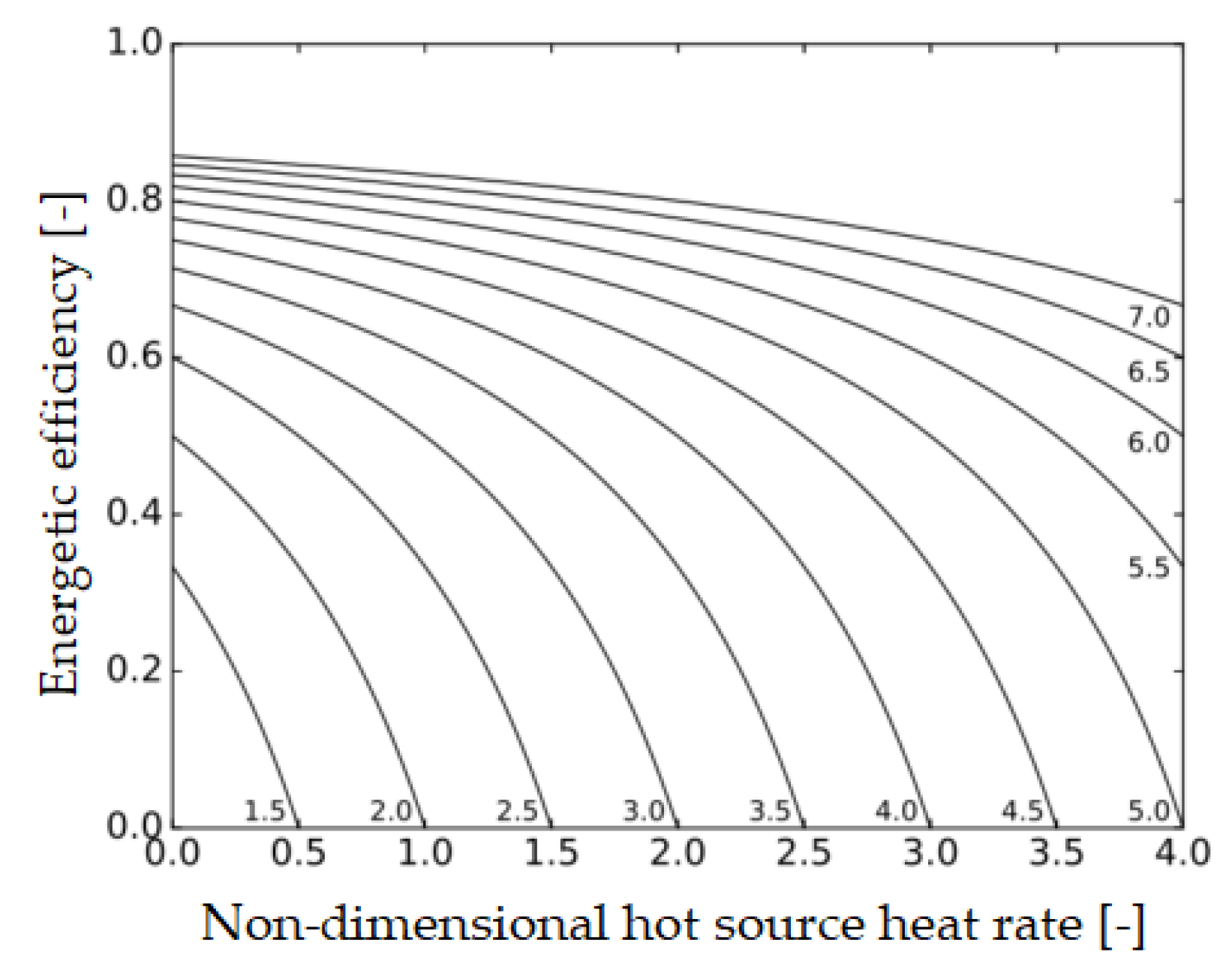
The first law efficiency at maximum power (Equation (21)) appears as a function of the non-dimensional heat rate ${\dot{q}}_0$ and a non-dimensional temperature t_HS such that:

$${\eta }_I\left({\dot{q}}_0,t_{HS} \right)=1-\frac{1}{t_{HS}\left(1-4·{\dot{q}}_0\right)},$$

(22)

with ${\dot{q}}_0 = \frac{{\dot{Q}}_0}{K_T·T_{HS}}$ and $t_{HS} = \frac{T_{HS}}{T_0}$.

The first law efficiency is represented (Figure 2) versus the non-dimensional hot source heat flux for different values of non-dimensional temperature t_HS. This figure shows a strong correlation between ${\dot{q}}_0$ and t_HS influences on efficiency, particularly in the practical range of use (low dimensional heat rate, relatively low value of t_HS).

To complete this approach, we consider an exergy analysis of the studied case. The available exergy in the case of latent heat is:

$$\dot{E}{x}_L = {\dot{Q}}_0\left(1-\frac{T_0}{T_{HS}}\right),$$

(23)

where the subscript L stands for latent heat.

Then, the endo-reversible Carnot exergetic efficiency is:

$${\eta }_{\dot{E}{x}_L}\left(Ma{x}_1\dot{W}\right) = \frac{Ma{x}_1\dot{W}}{\dot{E}{x}_L} = \frac{1-\frac{T_0}{T_{HS}-\frac{4·{\dot{Q}}_0}{K_T}}}{1-\frac{T_0}{T_{HS}}} = \frac{1-\frac{T_0}{T_{HS}\left(1-{\dot{4q}}_0\right)}}{1-\frac{T_0}{T_{HS}}}.$$

(24)

Equation (24) shows that the exergetic efficiency is a decreasing function of ${\dot{q}}_0$, that starts from 1 when ${\dot{q}}_0$ is equal to 0.

2.1.3. Chambadal’s Model: Endo-Reversible Case

The hypothesis of the Chambadal’s case is relative to the thermal contact at the cold sink that is considered perfect, which means that K_C is infinite and T_C = T₀. We maintain the imposed heat rate delivered by the heat source ${\dot{Q}}_H = {\dot{Q}}_0$ and the endo-reversibility hypothesis. In this case, by using Equations (1), (3) and (4), one gets:

$$\dot{W} = {\dot{Q}}_0\left(1-\frac{T_0}{T_H}\right),$$

(25)

with

$$T_H = T_{HS}-\frac{{\dot{Q}}_0}{K_H}.$$

(26)

By combining Equations (25) and (26), a new expression of the mechanical power is found:

$$\dot{W} = {\dot{Q}}_0\left(1-\frac{T_0}{T_{HS} - \frac{{\dot{Q}}_0}{K_H}}\right).$$

(27)

This form represents a particular expression of Equation (18) showing that $\dot{W}$ is zero for ${\dot{Q}}_0$ = 0 and ${\dot{Q}}_0 = K_H\left(T_{HS}-T_0\right)$. An optimum between these two values can be found by derivative with respect to ${\dot{Q}}_0$. After term rearrangement, one gets:

$${{\dot{Q}}_0}^{*} = K_H\sqrt{T_{HS}}\left(\sqrt{T_{HS}}-\sqrt{T_0}\right),$$

(28)

$$Max\dot{W} = K_H{\left(\sqrt{T_{HS}}-\sqrt{T_0}\right)}^2,$$

(29)

and

$${\eta }_I\left(Max\dot{W}\right) = 1-\sqrt{\frac{T_0}{T_{HS}}}.$$

(30)

These results are similar to those obtained in Section 2.1.1, with K_C tending to infinite. The particular form of the efficiency for imposed ${\dot{Q}}_0$ could be retrieved as:

$${\eta }_I\left({\dot{Q}}_0\right)=1-\frac{T_0}{T_{HS} - \frac{{\dot{Q}}_0}{K_H}}.$$

(31)

2.2. Sensible Heat Valorization for Finite Heat Source

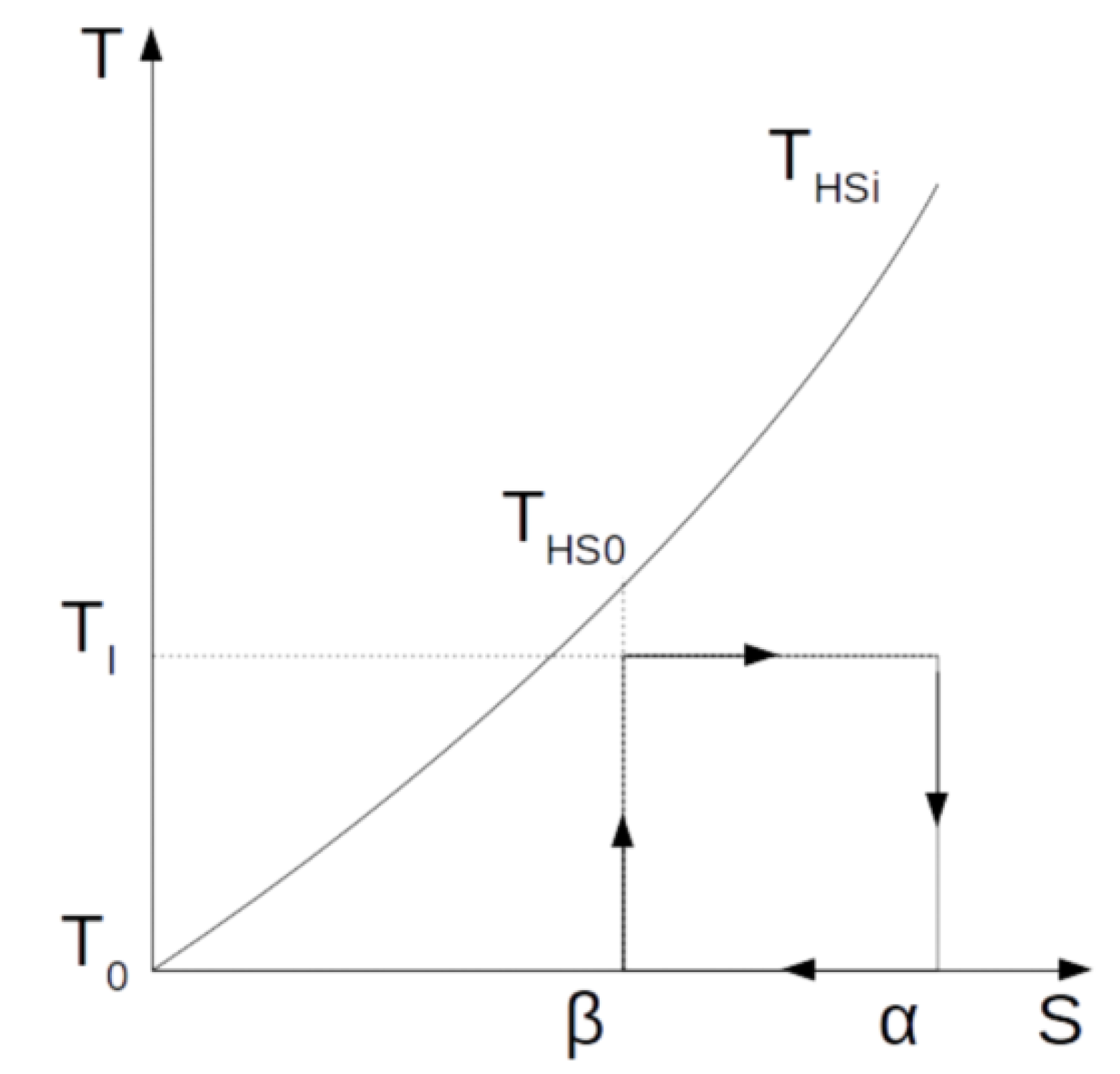
When considering the same hypotheses as in Section 2.1, the T–S diagram of Figure 3 is obtained, and it corresponds to sensible heat transfer case.

It can be observed this time that the recoverable sensible heat flux $\dot{Q_0}$ depends on the source fluid mass flow rate ${\dot{m}}_H$ and on its mass specific heat at constant pressure ${\overline{c}}_{p,H}$ (mean value over the temperature variation range [T₀, T_HSi]). Thus, the thermal capacity rate ${\dot{C}}_H$ equals:

$${\dot{C}}_H = {\dot{m}}_H·{\overline{c}}_{p,H}.$$

(32)

Then, the recoverable heat flux $\dot{Q_0}$ is deduced as:

$${\dot{Q}}_0 = {\dot{C}}_H·\left(T_{HSi}-T_0\right).$$

(33)

The Carnot engine is inserted between the evolving source temperature T_HS (with T₀ < T_HS < T_HSi) and the sink temperature T_CS (with T₀ < T_CS < T_CS0).

To simplify and determine only the superior upper bound, the Chambadal’s engine model (perfect heat transfer at the cold sink) is considered here as well. This approximation corresponds to an ambient cold capacity rate ${\dot{C}}_C = {\dot{m}}_C{\overline{c}}_{p,C}$ much higher than the hot thermal capacity rate ${\dot{C}}_H$ given by Equation (32) (which remains a reasonable hypothesis).

Consequently, the optimization consists in placing the endo-reversible Carnot cycle in an optimal way in the curvilinear triangle (T₀, T_HSi, α) to obtain the maximum mechanical power $\dot{W}$:

$$\dot{W} = {\dot{Q}}_0\left(1-\frac{T_0}{T_I}\right),$$

(34)

with

$${\dot{Q}}_{0 }= {ϵ}_H·{\dot{C}}_H\left(T_{HSi}-T_I\right) = {\dot{C}}_H\left(T_{HSi}-T_{HSo}\right),$$

(35)

where ε_H is the effectiveness of the high temperature heat exchanger and T_I is the vaporization temperature of the working fluid in the Carnot’s engine cycle.

Supposing that ε_H = 1, one gets T_HS0 equal to T_I as used by Chambadal in its Carnot cycle model. More generally, by combining Equations (32) and (33) we get:

$$\dot{W} = {ϵ}_H·{\dot{C}}_H\left(T_{HSi}-T_I\right)\left(1-\frac{T_0}{T_I}\right).$$

(36)

Furthermore, from the derivative with respect to T_I of Equation (36) equal to zero, the fluid optimal vaporization temperature $T_I^{*}$ is obtained:

$${T_I}^{*} = \sqrt{T_{HSi}·T_0}.$$

(37)

This result is formally close to the one obtained in Section 2.1, and $Max\dot{W}$ for the sensible heat case is deduced as:

$$Max\dot{W} = {ϵ}_H·{\dot{C}}_H{\left(\sqrt{T_{HSi}}-\sqrt{T_0}\right)}^2,$$

(38)

while the corresponding efficiency becomes:

$${\eta }_I\left(Max\dot{W}\right)=1-\sqrt{\frac{T_0}{T_{HSi}}}$$

(39)

This result is formally like the one obtained in Section 2.1.1 (see Equation (10)). However, some important differences appear, and they will be discussed in Section 3.

3. New Criteria Compared to Classical Approach

3.1. Optimum Mechanical Power Recovery for Chambadal’s Engine

The comparison of the optimum mechanical power expressions previously established by Equation (29) for the latent heat recovery:

$$Max{\dot{W}}_L = K_H{\left(\sqrt{T_{HS}}-\sqrt{T_0}\right)}^2,$$

and Equation (38) for the sensible heat recovery:

$$Max{\dot{W}}_S = {ϵ}_H·{\dot{C}}_H{\left(\sqrt{T_{HSi}}-\sqrt{T_0}\right)}^2,$$

emphasizes a strong analogy. Thus, the term ${\epsilon }_H{\dot{C}}_H$ corresponds to the finite physical dimension of the source K_H (with same unit), and the temperature T_HSi corresponds to T_HS. These two temperatures also appear in the expression of the first law efficiency at maximum power:

By Equation (30) for the latent heat case:

$${\eta }_{IL}\left(Max\dot{W}\right) = 1-\sqrt{\frac{T_0}{T_{HS}}},$$

By Equation (39) for the sensible heat case:

$${\eta }_{IS}\left(Max\dot{W}\right)=1-\sqrt{\frac{T_0}{T_{HSi}}}.$$

Although the two expressions show apparently the same form, they include differences that will be analyzed hereafter. Thus, the exergy analysis of the two heat recovery cases leads to different results regarding the exergetic efficiency. This difference has the origin in the way the heat transfer happens. Thus, if the analysis is straightforward for the latent heat case where the heat transfer by phase change of a pure substance occurs at constant temperature, it is not the same in the case of sensible heat, where even for constant thermophysical properties (not functions of temperature), an integration with respect to temperature appears (see Figure 3 and the developments in Section 3.2). Thereby, the sensible heat case deserves a careful examination hereafter.

3.2. Exergetic Efficiency for the Sensible Heat Recovery Case

The maximum recoverable heat exergy is:

$$\dot{E}x\left(T_{HSi},T_I\right) = \underset{T_I}{\overset{T_{HSi}}{{\displaystyle \int }}}{\dot{C}}_H\left(1-\frac{T_0}{T}\right)dT.$$

(40)

By integrating Equation (40), one gets:

$$\dot{E}x\left(T_{HSi},T_I\right) = {\dot{C}}_H\left(T_{HSi}-T_I\right)\left(1-\frac{T_0}{{\tilde{T}}_I}\right),$$

(41)

where ${\tilde{T}}_I$ is the entropic temperature defined by:

$${\tilde{T}}_I = \frac{H_{HSi}-H_I}{S_{HSi}-S_I} = \frac{T_{HSi}-T_I}{ln\frac{T_{HSi}}{T_I}}.$$

(42)

Therefore, the exergetic efficiency at maximum power in the Chambadal’s model is:

$${\eta }_{Ex}\left(T_{HSi},T_I{}^{*}\right)=\frac{{\left(\sqrt{T_{HSi}}-\sqrt{T_0}\right)}^2}{\sqrt{T_{HSi}}\left(\sqrt{T_{HSi}}-\sqrt{T_0}\right)-T_{0}ln\sqrt{\frac{T_{HSi}}{T_I{}^{*}}}}.$$

(43)

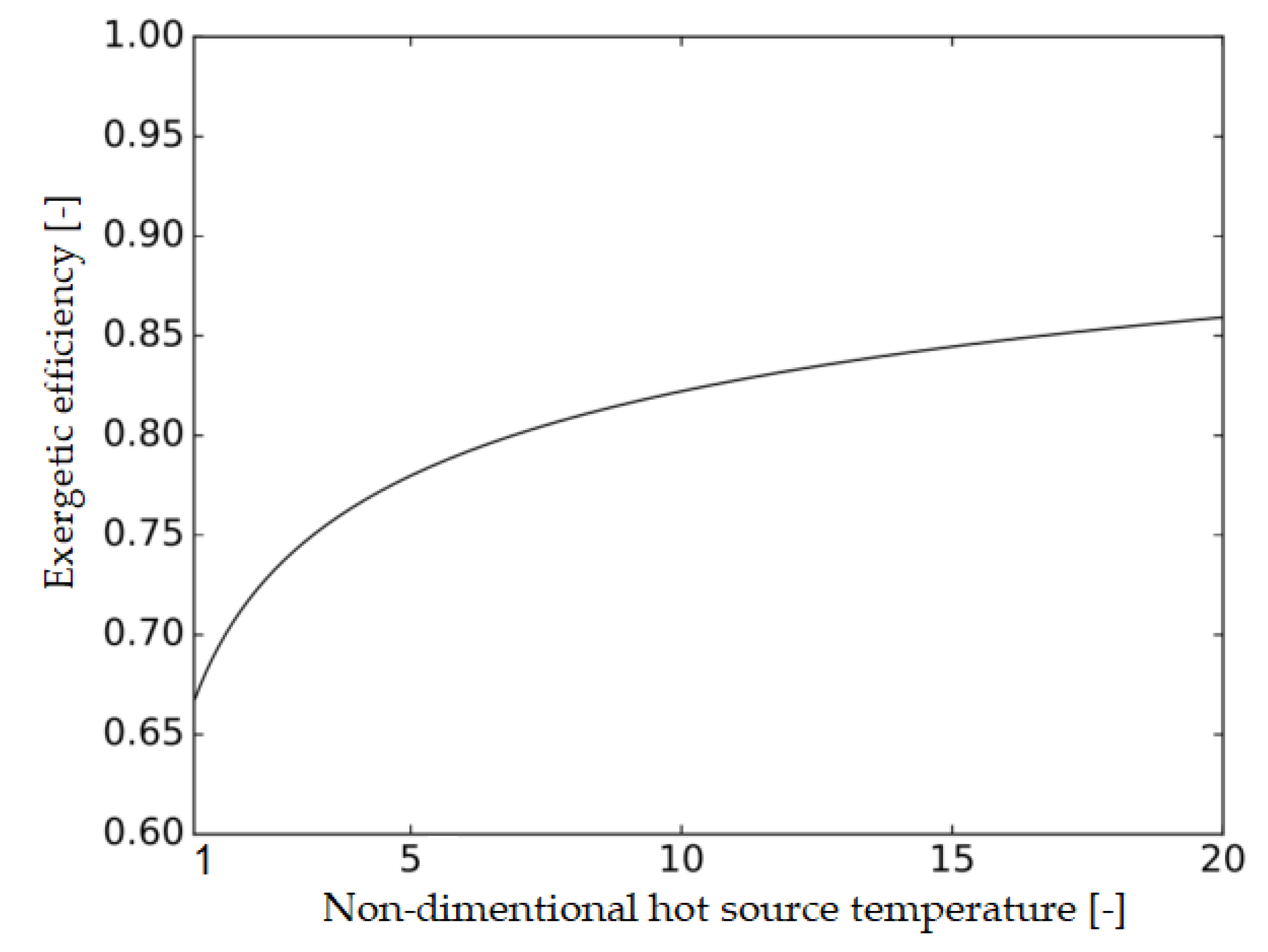
By using the non-dimensional temperatures with respect to T₀ (reference temperature), the new form of Equation (43) is:

$${\eta }_{Ex}\left(t_{HSi},t_I{}^{*}\right)=\frac{{\left(\sqrt{t_{HSi}}-1\right)}^2}{\sqrt{t_{HSi}}\left(\sqrt{t_{HSi}}-1\right)-ln\sqrt{t_{HSi}}}.$$

(44)

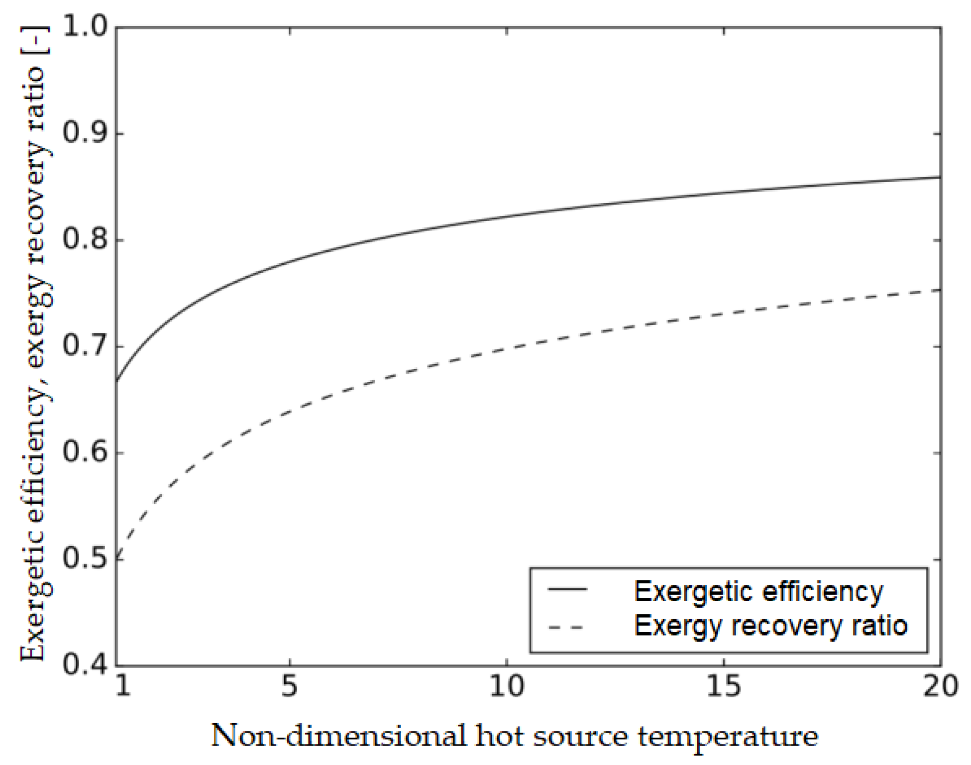
The variation of the exergetic efficiency versus the non-dimensional heat source temperature is illustrated in Figure 4. It shows that exergetic efficiency is an increasing function of t_HSi with an asymptotic behavior.

The use of L’Hospital’s rule allows us to get the lower limit of the exergetic efficiency, namely 0.67, that corresponds to t_HSi = 1. For the physical domain of t_HSi from 1 to 5, one notes a significant increase of the exergetic efficiency with t_HSi (from 0.67 to 0.77).

3.3. Recovery Ratios

These new criteria are defined as the ratio of the maximum recoverable power divided by the energy rate or exergy rate available between the heat source and the ambient. They characterize the whole system consisting of the heat source and converter.

In the present approach the recovery ratios study is limited to the sensible heat case.

3.3.1. Energy Recovery Ratio for the Sensible Heat Case

This ratio τ_ES is defined as the sensible heat rate recovered divided by the available sensible heat:

$${\tau }_{ES} = \frac{{\dot{C}}_H\left(T_{HSi}-T_I\right)}{{\dot{C}}_H\left(T_{HSi}-T_0\right)}.$$

(45)

At maximum power conditions, one gets:

$${\tau }_{ES}{}^{*} = \frac{\sqrt{T_{HSi}}}{\sqrt{T_{HSi}}+\sqrt{T_0}}.$$

(46)

By using the non-dimensional temperature of the heat source in Equation (46), a straightforward expression yields as:

$${\tau }_{ES}{}^{*} = \frac{\sqrt{t_{HSi}}}{\sqrt{t_{HSi}}+1}.$$

(47)

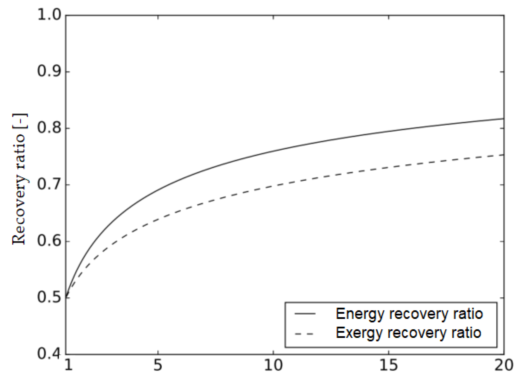
The energy recovery ratio versus the non-dimensional temperature of the heat source is illustrated in Figure 5.

One notes that the energy recovery ratio at maximum power is continuously increasing with non-dimensional heat source temperature t_HSi, thus more interesting as t_HSi is higher.

3.3.2. Exergy Recovery Ratio for the Sensible Heat Case

The exergy recovery ratio τ_Ex is defined as the exergy recovery (namely the mechanical power) divided by the whole available exergy at the source:

$${\tau }_{Ex} = \frac{exergy recovery}{available exergy}.$$

(48)

For latent heat recovery case and maximum power conditions, Equation (48) leads to the expression in Equation (24).

Hence, Equation (24) illustrates that the exergy recovery ratio is identical to the exergetic efficiency. It is also a decreasing function of ${\dot{Q}}_0$, even if demonstrated for the endoreversible situation.

For sensible heat case, the exergy recovery ratio τ_ExS becomes:

$${\tau }_{ExS}\left(Max\dot{W}\right) = \frac{{\dot{C}}_H{\left(\sqrt{T_{HSi}}-\sqrt{T_0}\right)}^2}{\dot{Ex}\left(T_{HSi},T_0\right)},$$

(49)

where

$$\dot{Ex}\left(T_{HSi},T_0\right) = {\dot{C}}_H\left(T_{HSi}-T_0\right)\left(1-\frac{T_0}{\widetilde{T_0}}\right),$$

(50)

with

$${\tilde{T}}_0 = \frac{T_{HSi}-T_0}{ln\frac{T_{HSi}}{T_0}}.$$

(51)

Hence, the exergy recovery ratio of sensible heat becomes:

$${\tau }_{ExS}\left(Max\dot{W}\right) = \frac{{\left(\sqrt{T_{HSi}}-\sqrt{T_0}\right)}^2}{T_{HSi}-T_0-T_0·ln\frac{T_{HSi}}{T_0}},$$

(52)

or in the non-dimensional form with respect to T₀:

$${\tau }_{ExS}\left(Max\dot{W}\right) = \frac{{\left(\sqrt{t_{HSi}}-1\right)}^2}{t_{HSi}-1-ln\left(t_{HSi}\right)}.$$

(53)

The sensible heat exergy recovery ratio is plotted versus the non-dimensional source temperature for the sensible heat case in Figure 5.

The comparison of the energy and exergy recovery ratios (Figure 5) clearly shows that the exergy recovery ratio is lower than the energy one. The curves start at the same point but diverge when the non-dimensional heat source temperature increase. For the upper value of the non-dimensional temperature of heat source, the relative difference between the two ratios is significant. Thus, an increase from 0.70 to 0.77 is noted at $t_{HSi}$ = 10, which means a relative leap of nearly 10%.

An important consequence relative to sensible heat recovery in the frame of the chosen hypotheses is that the exergetic efficiency (Equation (44)) at maximum power ${\eta }_{ex}\left(t_{HSi},t_I{}^{*}\right)$ is different from the exergy recovery ratio ${\tau }_{ExS}\left(Max\dot{W}\right)$ (Equation (53)). This difference is illustrated in Figure 6, which shows the exergetic efficiency being favorable, but not representative of the exergy recovery. The absolute difference is decreasing when t_HSi increases, i.e., from 0.18 to half the value near of t_HSi = 10. Consequently, the evaluation of the waste heat recovery by the exergetic efficiency turns out to be too optimistic by a relative order of 30%.

4. Conclusions and Perspectives

Waste heat recovery can be achieved through two main forms: the latent heat and sensible heat. These two forms were analyzed in the present paper, leading to the identification of some specific aspects, mainly the definition of the entropic temperature in the case of sensible heat recovery.

The thermomechanical recovery of waste heat was examined by considering a Carnot endo-reversible model, and Chambadal’s engine model, with a constant temperature of the hot reservoir. Maximum recoverable power and corresponding first law efficiency of exergy efficiency were exemplified for constant temperature heat reservoirs.

To demonstrate its feasibility of the sensible heat recovery, the limit case of the Chambadal’s model, where the cold reservoir is supposed to be a thermostat (infinite sink) at the ambient temperature T₀, was considered. It allowed establishing an upper bound to the recovery of the sensible heat. Thus, the total recovery of the waste heat flux is not possible for the case of sensible heat even in the case of the Carnot cycle, while it can be completed for the latent heat. This is an important result, since most recoverable thermal wastes are sensible heat.

The results of the study have also emphasized that at maximum power regime of the engine, the efficiency according to the first law of thermodynamics, or the exergetic efficiency, are not truly representative criteria for the complete characterization of technologies used for waste heat valorizing.

Our proposal of two new criteria called “recovery ratio” refers either to maximum recoverable energy on heat form (independently of process), τ_ES, or to maximum recoverable exergy, τ_Ex. In the case of the latent heat, the last ratio is identical to the exergetic efficiency at maximum power conditions. However, it is not the case for sensible heat, mainly due to the non-used exergy between T_I* chosen as high temperature for the Carnot cycle and T₀, the low temperature (ambient).

The importance of our proposal is clearly shown in Figure 5 by the energy recovery ratio that overestimates the process when compared to the exergy recovery ratio. Moreover, the interest of the exergetic recovery ratio appeared in Figure 6 where the exergetic efficiency alone lead to an overestimation of the waste heat valuation by about 30%. Therefore, our proposal of criteria shows that in the most common case of sensible heat recovery, the exergy recovery ratio approach should be preferred in order to have a better estimate of the recovery process quality.

These new criteria may help to wisely choose the technical solutions for efficient recovery of waste heat by different technologies.

Further development of this work consists of extending the new criteria used to other configurations analysis and to a comparison of existing systems and processes performance.

References

- Durakovic, G.; Skaugen, G. Analysis of thermodynamic models for simulation and optimization of Organic Rankine Cycles. Energies 2019, 12, 3307. [Google Scholar] [CrossRef] [Green Version]
- Valencia, G.; Fontalvo, A.; Cardenas, Y.; Duarte, J.; Isaza, C. Energy and exergy analysis of different exhaust waste heat recovery systems for natural gas engine based on ORC. Energies 2019, 12, 2378. [Google Scholar] [CrossRef] [Green Version]
- Huang, S.; Li, C.; Tan, T.; Fu, P.; Xu, G.; Yang, Y. An improved system for utilizing low-temperature waste heat of flue gas from coal-fired power plants. Entropy 2017, 19, 423. [Google Scholar] [CrossRef] [Green Version]
- Feidt, M.; Costea, M. Energy and exergy analysis and optimization of combines heat and power systems. Comparison of various systems. Energies 2012, 5, 3701–3722. [Google Scholar] [CrossRef] [Green Version]
- Brückner, S.; Liu, S.; Miró, L.; Radspieler, M.; Cabeza, L.F.; Lävemann, E. Industrial waste heat recovery technologies: An economic analysis of heat transformation technologies. Appl. Energy 2015, 151, 157–167. [Google Scholar] [CrossRef]
- Zhang, Q.; Zhao, X.; Lu, H.; Ni, T.; Li, Y. Waste energy recovery and energy efficiency improvement in China’s iron and steel industry. Appl. Energy 2017, 191, 502–520. [Google Scholar] [CrossRef]
- Agathokleous, R.; Bianchi, G.; Panayiotou, G.; Arestia, L.; Argyrou, M.C.; Georgiou, G.S.; Tassou, S.A.; Jouhara, H.; Kalogirou, S.A.; Florides, G.A.; et al. Waste heat recovery in the EU industry and proposed new technologies. Energy Procedia 2017, 161, 489–496. [Google Scholar] [CrossRef]
- Bell, L.E. Cooling, heating, generating power, and recovering waste heat with thermoelectric systems. Science 2008, 321, 1457–1461. [Google Scholar] [CrossRef] [PubMed] [Green Version]
- Le, V.L. Étude de la Faisabilité des Cycles Sous-Critiques et Supercritiques de Rankine Pour la Valorisation de Rejets Thermiques. Ph.D. Thesis, Lorraine University, Lorraine, France, September 2014. (In French). [Google Scholar]
- Glavatskaya, O.; Goupil, C.; El Bakkali, A.; Shonda, O. Exergetic analysis of a thermogenerator for automotive application: A dynamic numerical approach. AIP Conf. Proc. 2012, 1449, 475–481. [Google Scholar]
- Glavatskaya, O. Conversion D’énergie Thermique en Energie Electrique Par Les Modules Thermoélectriques en Vue de Réduire La Consommation et Les Emissions Polluantes. Ph.D. Thesis, University of Caen, Caen, France, January 2012. (In French). [Google Scholar]
- Glavatskaya, Y. Conversion de L’énergie Thermique Des Gaz D’échappement en Travail Mécanique Par un Cycle de RANKINE Afin de Réduire Les Emissions Des Gaz à Effet de Serre. Ph.D. Thesis, University Paris 6, Paris, France, January 2012. (In French). [Google Scholar]
- Dong, Y.; El-Bakkali, A.; Feidt, M.; Descombes, G.; Périlhon, C. Association of finite-dimension thermodynamics and a bond-graph approach for modeling an irreversible heat engine. Entropy 2012, 14, 1234–1258. [Google Scholar] [CrossRef] [Green Version]
- Anton, S.R.; Sodano, H.A. A review of power harvesting using piezoelectric materials (2003–2006). Smart Mater. Struct. 2007, 16, 3. [Google Scholar]
- Chagnon-Lessard, N.; Mathieu-Potvin, F.; Gosselin, L. Geothermal power plants with maximized specific power output: Optimal working fluid and operating conditions of subcritical and transcritical Organic Rankine Cycles. Geothermics 2016, 64, 111–124. [Google Scholar] [CrossRef]
- Rachedi, M.; Feidt, M.; Amirat, M.; Merzouk, M. Optimal operating conditions of a transcritical endoreversible cycle using a low enthalpy heat source. Appl. Therm. Eng. 2016, 107, 379–385. [Google Scholar] [CrossRef]
- Le, V.L.; Feidt, M.; Kheiri, A.; Pelloux-Prayer, S. Performance optimization of low-temperature power generation by supercritical ORCs (Organic Rankine Cycles) using low GWP (global warming potential) working fluids. Energy 2014, 67, 513–526. [Google Scholar] [CrossRef]
- Eveloy, V.; Karunkeyoon, W.; Rodgers, P.; Al Alili, A. Energy, exergy and economic analysis of an integrated solid oxide fuel cell—Gas turbine—Organic Rankine power generation system. Int. J. Hydrogen Energy 2016, 41, 13843–13858. [Google Scholar] [CrossRef]
- Calise, F.; d’Accadia, M.D.; Macaluso, A.; Piacentino, A.; Vanoli, L. Exergetic and exergoeconomic analysis of a novel hybrid solar-geothermal polygeneration system producing energy and water. Energy Convers. Manag. 2016, 115, 200–220. [Google Scholar] [CrossRef]
- Chen, L.G.; Meng, F.K.; Sun, F.R. Thermodynamic analyses and optimization for thermoelectric devices: The state of the arts. Sci. China Technol. Sc. 2016, 59, 442–455. [Google Scholar] [CrossRef]
- Oluleye, G.; Jobson, M.; Smith, R.; Perry, S.J. Evaluating the potential of process sites for waste heat recovery. Appl. Energy 2016, 161, 627–646. [Google Scholar] [CrossRef]
- Singh, D.V.; Pedersen, E. A review of waste heat recovery technologies for maritime applications. Energy Convers. Manag. 2016, 111, 315–328. [Google Scholar] [CrossRef]
- Punov, P.; Milkov, N.; Danel, Q.; Périlhon, C. A Study of Waste Heat Recovery Impact on a Passenger Car Fuel Consumption in New European Driving Cycle. In Proceedings of the European Automotive Congress EAEC-ESFA 2015, Bucharest, Romania, 25–27 November 2015; pp. 151–163. [Google Scholar]
- Danel, Q. Étude Numérique et Expérimentale D’un Cycle de Rankine-Hirn de Faible Puissance Pour la Récupération D’énergie. Ph.D. Thesis, CNAM, Paris, France, December 2016. (In French). [Google Scholar]
- Curzon, F.L.; Ahlborn, B. Efficiency of a Carnot engine at maximum power output. Am. J. Phys. 1975, 43, 22–24. [Google Scholar] [CrossRef]
- Feidt, M. Thermodynamique Optimale en Dimensions Physiques Finies; Lavoisier: Paris, France, 2013. (In French) [Google Scholar]
Figure 1.
Representation for latent heat recovery by means of a Carnot cycle in a T–S diagram.
Figure 2.
Energy efficiency versus non-dimensional hot heat rate for different non-dimensional temperature.
Figure 3.
Scheme for sensible heat recovery by means of a Carnot cycle illustrated in T–S diagram.
Figure 4.
Exergetic efficiency versus heat source non-dimensional temperature.
Figure 5.
Energy and exergy recovery ratio for sensible heat case versus the non-dimensional heat source temperature.
Figure 6.
Exergetic efficiency and exergy recovery ratio for sensible heat case versus the non-dimensional heat source temperature.
© 2020 by the authors. Licensee MDPI, Basel, Switzerland. This article is an open access article distributed under the terms and conditions of the Creative Commons Attribution (CC BY) license (http://creativecommons.org/licenses/by/4.0/).
Share and Cite
MDPI and ACS Style
Feidt, M.; Costea, M.; Feidt, R.; Danel, Q.; Périlhon, C. New Criteria to Characterize the Waste Heat Recovery. Energies 2020, 13, 789. https://doi.org/10.3390/en13040789
AMA Style
Feidt M, Costea M, Feidt R, Danel Q, Périlhon C. New Criteria to Characterize the Waste Heat Recovery. Energies. 2020; 13(4):789. https://doi.org/10.3390/en13040789
Chicago/Turabian StyleFeidt, Michel, Monica Costea, Renaud Feidt, Quentin Danel, and Christelle Périlhon. 2020. "New Criteria to Characterize the Waste Heat Recovery" Energies 13, no. 4: 789. https://doi.org/10.3390/en13040789
Note that from the first issue of 2016, this journal uses article numbers instead of page numbers. See further details here.