Configuration Optimization Model for Data-Center-Park-Integrated Energy Systems under Economic, Reliability, and Environmental Considerations

Abstract

The analysis of energy configuration in the planning of data-center-park-integrated energy systems (DCP-IESs) has become an enormous challenge, owing to multi-energy complementarity, energy cascade use, and energy security. In this study, a configuration model of DCP-IESs was established to obtain the economic and low-carbon energy uses of the data centers, based on mixed integer linear programming. In the model, carbon emissions were converted to economic indicators through carbon pricing. Then, the configuration model was modified according to the security of the proposed device switching logic, and the Markov-based reliability estimation method was used to ensure the redundant design of the configuration. Using the new energy configuration method, the DCP-IES configuration scheme could be obtained under economical, low-carbon, and high reliability conditions. A data center park in Shanghai was selected as a case study, and the results are as follows: it will only take 2.88 years for the economics of DCP-IES to reach those of traditional data center energy systems. Additionally, the use of configuration model in DCP-IES would result in a reduction in annual carbon emissions of 39,323 tons, with a power usage effectiveness of 1.388, whereas an increase in reliability results in an increasingly faster increase in the initial investment cost.

1. Introduction

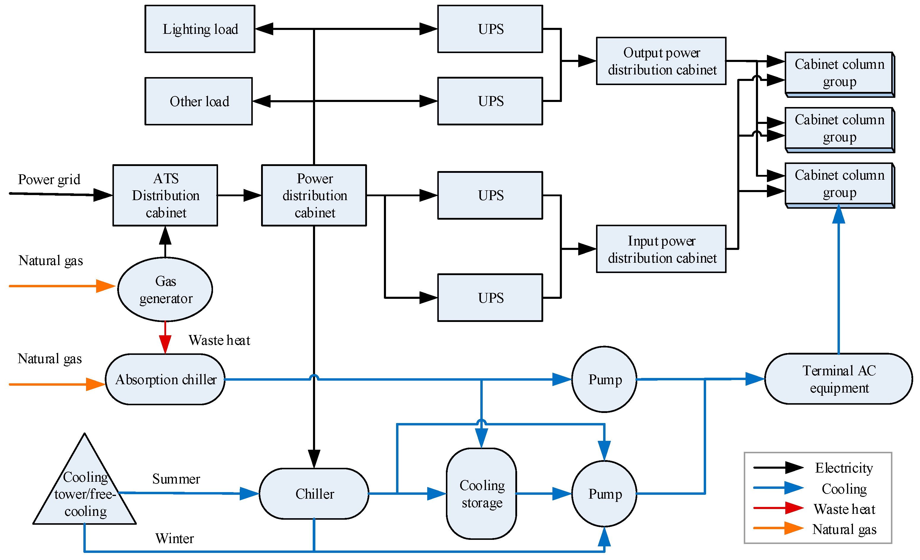
1.1. DCP-IESs and Their Key Characteristics

With advancements in industrialization and informatization, large data centers, which are usually distributed in the form of a park, are expanding rapidly in China. The market size of Internet Data Centers (IDCs) in China and the world is shown in Figure 1 [1], reflecting a clear trend of rapid increase in recent years (average rate of increase is 40% in China). Along with this rapid development, high energy consumption and carbon emissions have become a major problem for IDCs [2]. The existing research [3] shows that the reasonable configuration of data-center-park-integrated energy systems (DCP-IES) can realize economical, low-carbon, and reliable operation. Therefore, it is urgent to establish a better model for optimizing the energy configuration and analyzing the reliability of DCP-IES to reduce both energy consumption and carbon emissions.

Data center energy consumption involves not only consumption from web servers and private branch exchanges but also consumption from air conditioning systems (ACS), power distribution units, uninterrupted power supplies (UPS), and illuminating and switching units [4]. Figure 2 shows the energy consumption structure of IDCs, most energy consumption of which is attributed to the use of traditional electrical chiller system [5]. From Figure 2, the energy consumption structure of IDCs in China and the world is basically the same, and there are primarily two components of energy consumption: electrical consumption from IT equipment and energy consumption from other auxiliary equipment. IT equipment consumes approximately 50% of the total energy, whereas ACS equipment consumes nearly 35%, with a power usage effectiveness (PUE) [4] of approximately 2. This demonstrates the first key characteristic of DCP-IESs: high energy consumption. PUE is defined as the ratio of total power consumption of IDC to IT power load, as shown in Equation (1) [6], where $P_e$ is the input power, which includes the large power grid and renewable energy generation; $P_{oil}$ is the input oil; $P_{gas}$ is the input gas; $P_c$ is the input cooling; and $P_{IT}$ is the power consumption of IT equipment. The units of the above variables are electricity-equivalent units. The higher the PUE value is, the lower the efficiency of the IDC [7].

$$PUE=\frac{{\displaystyle \sum }{P}_e+{\displaystyle \sum }{P}_{oil}+{\displaystyle \sum }{P}_{gas}+{\displaystyle \sum }{P}_c}{{\displaystyle \sum }{P}_{IT}},$$

(1)

On the one hand, most energy consumed by DCP-IESs originates from the state power grid, with a carbon emission factor 0.620 (tCO₂/MWh) in China, as shown in

Table 1. Carbon emission factor of electric power industry in the world [8].

Electric Power Industry	Carbon Emission Factor (tCO2/MWh)
China (2017)	0.620
USA (2017)	0.420
UK (2017)	0.237
Germany (2016)	0.560
France (2017)	0.074
Japan (2016)	0.544
Russia (2016)	0.358
India (2017)	0.723

[8]. This demonstrates the second key feature of DCP-IESs: high carbon emissions. Additionally, IDCs exhibit a cascade energy use structure, e.g., IT equipment generally consumes high-grade energy, whereas cooling equipment uses low-grade energy [9].

1.2. Literature Review

For the three key characteristics described above, scholars carried out numerous studies. Generally, the low-carbon emissions, low energy consumption, and cascade energy use of data centers can be achieved through the operational efficiency optimization of the equipment and the optimal design of energy system.

For the operational efficiency optimization of the equipment, an attempt to maximize the operational efficiency of the equipment is typically conducted by increasing the fuel conversion efficiency, optimizing the operational control strategy, etc. Rong [4] reviewed three methods to reduce the energy consumption of IDCs: (1) using energy-saving technologies in high-performance computing, (2) implementing energy conservation technologies in computer rooms, and (3) applying renewable energy. Rossi [10] indicated that several techniques could be used to promote energy efficiency in high-performance computing, ranging from scaling the frequencies of the processors to putting the device to sleep during idle periods and consolidating virtual machines. Additionally, supercomputer architecture, parallel science, and parallel software development can provide opportunities for energy conservation [11,12,13,14]. For energy conservation of ACS, there are four main considerations: (1) appropriate cooling strategy [15]; (2) good layout design and air flow distribution for computer rooms [16,17]; (3) economizer cycles [18,19]; and (4) simulation-based control [20]. In addition to these, the use of heat pipes [5,21,22,23] and free-cooling [24,25,26] in data centers was also attempted. All of the above-mentioned methods involved the optimization of the method or improvement of a specific technology in existing energy systems; however, they did not address configuration optimization in the system planning and design.

For the optimal design of energy system, in order to integrate multiple energy sources and increase renewable energy penetration, scholars mainly adopt three methods to optimize the design of energy system: (1) classic methods, (2) metaheuristic methods, and (3) distributed computing. Sheme et al. [27] introduced the minimum percentage supply (MPS) and used the classic algorithms to configure the capacity of wind power and photovoltaic power in data center, which maximized the renewable energy use in high latitudes. Wang et al. [28] developed a multi-objective optimal design model for integrated energy system with economy, technology, and environment minimization. Then the configuration capacity of various equipment was obtained by using the non-dominated sorting genetic algorithm 2 (NSGA-II). Tran et al. [29] conducted the alternating direction method of multipliers (ADMM) to deal with the typical daily optimal dispatching problem of combined heating and power (CHP) system. The case study showed that ADMM algorithm had the faster convergence speed than particle swarm optimization (PSO). van der Heijde et al. [30] developed a two-stage optimization algorithm to achieve the optimal design and dispatching of integrated heating system. The genetic algorithm (GA) was adopted to realize the equipment capacity configuration in the first layer, and the optimization solution toolbox of Python was used to achieve the optimal dispatching of the equipment in the second layer. Reynolds et al. [31] developed an optimized dispatching management method, in which the artificial neural network (ANN) and the GA were adopted to predict the output of renewable energy equipment and determine the operation strategy of the equipment, respectively. In these studies, however, the strategy used at the operational stage was not combined with the selection of energy conversion technologies at the design stage, and the safety of the device pre-start and reliability of the system were not considered.

On the other hand, in the design of a DCP-IES, the reliability of the energy supply is very important [32], as any equipment failure may cause instability or even failure of the entire energy system. To improve the reliability of the DCP-IES, standby devices are typically provided [33]. However, this involves increasing the initial investment. In particular, after a certain increase in the reliability of the energy supply, a further small increase may require a huge investment [34]. Therefore, how to optimize the design configuration of standby devices has become an urgent issue in need for a solution. Additionally, the configuration of the DCP-IES by the method of multi-energy complementarity ultimately results in the increase in the switching frequency between devices [35]. In actual engineering applications, the device cannot immediately advance to its stable operational state, e.g., absorption chillers need approximately 40 min from start-up to smooth operation [35]. A normal energy supply can be guaranteed by the appropriate device switching logic when the device is switched. Therefore, it is necessary to design the relevant switching logic and analyze the possible system faults caused by the device switching. Then, the relevant constraints to avoid those faults are fed back into the configuration model to repair and improve the model.

In summary, there is no study on the configuration optimization model for DCP-IESs under multi-energy complementarity, device switching, and redundant design considerations. Therefore, it is significant to develop the configuration optimization model for DCP-IESs.

1.3. Scientific Contribution of the Study

Compared to previous research, the study aims to develop a new configuration optimization model for DCP-IESs under economic, environmental, and reliability considerations. Therefore, the major contributions of present work are listed as follows:

First, the integrated configuration model of DCP-IES was established based on mixed integer linear programming algorithms (MILP), considering both the cost and carbon emissions. A double-objective function was established by introducing carbon trading prices. In the model, the strategies for the operational stage were taken into consideration in the configuration of energy conversion technologies at the planning stage.

Second, compared with traditional electric cooling and large power grids powering, the multi-energy configuration increases the switching frequency between devices. The switching logic of the DCP-IES uninterrupted energy supply was implemented to ensure the system security during the frequent switching of the devices, given the pre-start time of the device, and the security constraints were fed back into the integrated configuration model. It is unique in current research.

Third, the reliability estimation method for the complex series-parallel energy system, based on Markov processes, enabled providing the redundant design of the modified optimization configuration to ensure that the DCP-IES was safe and reliable in the event of device failure. The logical structure of the study is shown in Figure 3. In summary, this study provided a method for the configuration of DCP-IESs in the planning and design stages under economic, environmental, and high reliability considerations.

This paper contains five different sections: Section 1 provides an introduction of the DCP-IES from the research perspective and presents several characteristics of the DCP-IES; Section 2 describes the gaps in research of the current energy configuration of the DCP-IES; Section 3 describes the optimal configuration model and provides reliability calculation methods for the cooling and power supply systems in the new configuration model; Section 4 addresses a case study in Shanghai, China, which mainly includes model solving, model modification, result reliability analysis, and redundant design; and finally, the conclusions of this study are found in Section 5.

2. Existing Problems to Solve

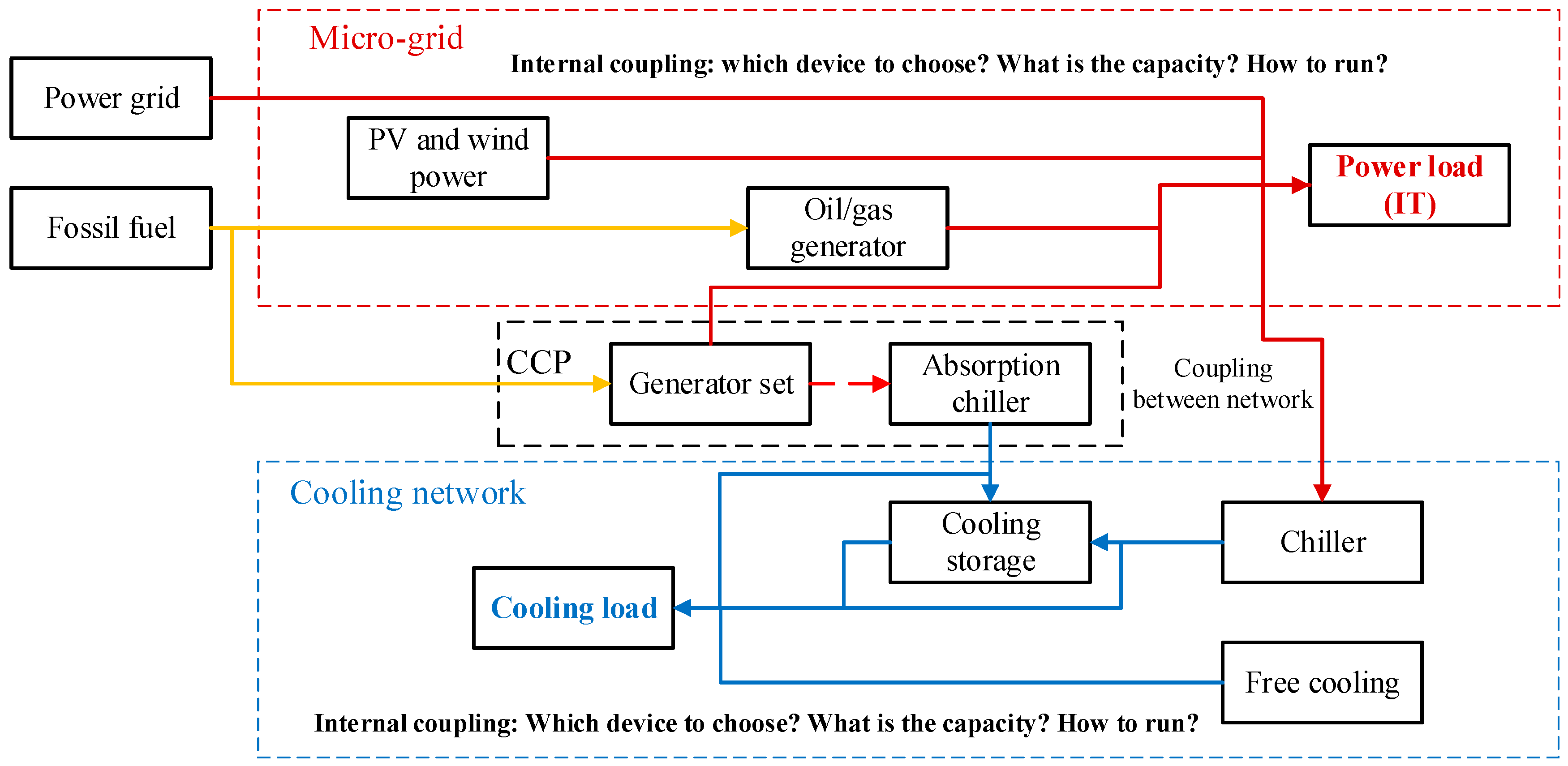
2.1. Three Coupled Configuration Issues

Basically, there are three major configuration issues in the DCP-IES: selection of energy conversion technologies, configuration capacity of each technology, and scheduling in the planning and design stages. These issues are coupled with each other within each energy network (cooling network and microgrid) or between networks (network nodes) and are difficult to segment, as shown in Figure 4. After solving these three issues, it will be easy to verify energy planning indexes, such as the total energy consumption index, carbon emission index, renewable energy index, and energy efficiency index, for IDC parks. This study provides a solution for these three problems by establishing a configuration model for the planning and design stages.

2.2. Redundancy and Device Switching Problems

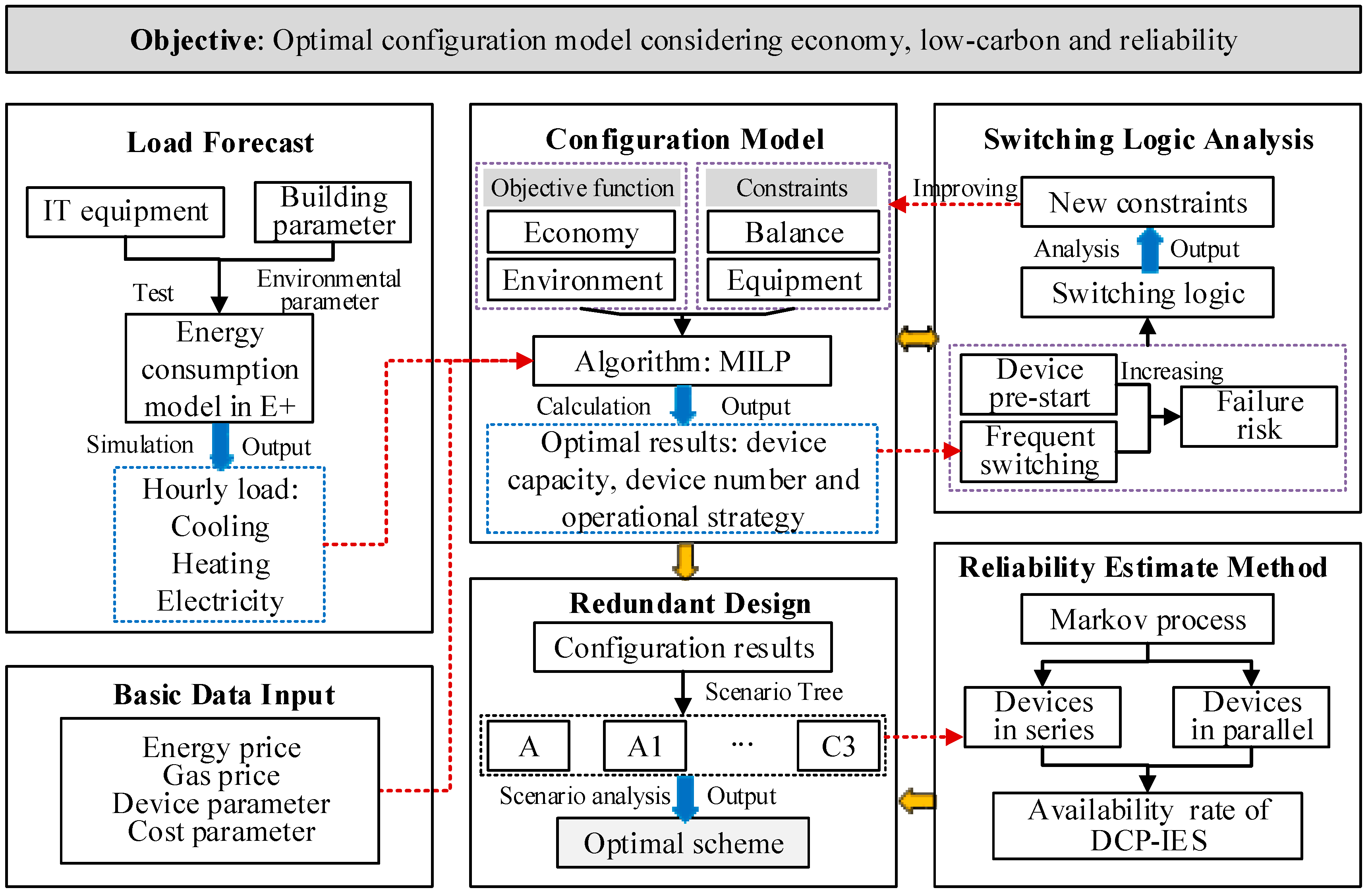
Compared with the traditional configuration, this new energy configuration model for DCP-IESs is more complicated. Complex device coupling and switching increases the probability of system failure. The comprehensive consideration of the DCP-IES energy supply reliability during the energy configuration phase is particularly important. Therefore, it is necessary to design a new redundant configuration method and switching logic to satisfy the security requirements of DCP-IESs. In this study, the evaluation of system reliability under the new energy configuration method primarily included two considerations: (1) possible system faults caused by the device switching would be analyzed, and the relevant constraints would be used to improve the configuration model; and (2) the reliability of the electricity and cooling redundant design would be analyzed based on Markov Chain processes.

3. Methodology

3.1. Hypotheses

Owing to the complexity of the energy system configuration process, assumptions were adopted by the model as follows: power from local generation is grid-connected without power injection and the step size of the dispatch with regard to cooling and power is one hour.

3.2. Configuration Model

Considering both the cost and carbon emissions, the objective function of the configuration model is defined in Equation (2), in which the optimal object of low-carbon emissions is transformed to economic objects through the carbon trading price. The variables are the output of each energy conversion technology at each hour, as shown in Equation (3), where $\mathit{P}$ is the variable matrix, $t=1,2,3,\dots ,8760$ represents the hour number over an entire year, $j$ represents the different energy conversion technologies listed in

Table 2. Energy conversion technologies.

$\mathit{j}$	1	2	3	4	5	6	7	8
Energy conversion technology	CCP	Absorption chiller	Chiller	Free-cooling	Cooling storage	Power grid	PV	Wind power

, and $p_{t,j}$ represents the output of $j$ at time $t$. Therefore, the final configured capacity can be defined as $\max \left(p_{t,j}\right)$.

$$\min {{\displaystyle \sum }}^{ }\left[C_{in}+C_o+C_m+{{\displaystyle \sum }}_{t=1}^{8760}\epsilon (p_{t,6}{\omega }_6+\frac{p_{t,1}}{{\eta }_{e}q}{\omega }_1)\Delta t\right],$$

(2)

$$\mathit{P}=\left[\begin{array}{cccc}{p}_{1,1}& p_{1,2}& \dots & p_{1,j}\\ p_{2,1}& p_{2,2}& \dots & p_{2,j}\\ ⋮& ⋮& ⋮& ⋮\\ p_{t,1}& p_{t,2}& \dots & p_{t,j}\end{array}\right],$$

(3)

where $C_{in}$ is the uniform annual value of the initial cost in USD and is defined by Equation (4), $C_o$ is the annual operative cost in USD and is defined by Equation (5), $C_m$ is the equipment maintenance cost in USD and is defined by Equation (6), $\epsilon$ is the carbon trading price, i.e., $4.71/tCO₂, ${\omega }_6$ is the carbon emission factor of power grid in tCO₂/kWh, ${\omega }_1$ is the carbon emission factor of natural gas in tCO₂/Nm³, ${\eta }_e$ is the generating efficiency of CCP in %, $q$ is the lower calorific value of natural gas in kJ/Nm³, and $\Delta t$ is the time interval in h.

$$C_{in}={{\displaystyle \sum }}_{j}P{r}_j\max \left(p_{t,j}\right)\frac{i}{1-\frac{1}{{\left(1+i\right)}^{n_j}}},$$

(4)

$$C_o={{\displaystyle \sum }}_{t=1}^{8760}P{r}_e\frac{100\ast p_{t,1}}{{\eta }_{e}q}\Delta t+P{r}_g{{\displaystyle \sum }}_{t=1}^{8760}{p}_{t,6}\Delta t+C_{trans},$$

(5)

$$C_m={{\displaystyle \sum }}_j[{\alpha }_j\max \left(p_{t,j}\right)+{\beta }_j({{\displaystyle \sum }}_{t=1}^{8760}{p}_{t,j}\Delta t)],$$

(6)

where $P{r}_j$ is the price per unit capacity of j in $/kW, $i$ is the dimensionless discount rate, $n_j$ is the service life of j in year, $P{r}_e$ is the time-of-use electricity price in $/kWh, $P{r}_g$ is the natural gas price in $/Nm³, $C_{trans}$ is the basic power cost of transformer in USD, ${\alpha }_j$ is the dimensionless fixed cost factor of j, and ${\beta }_j$ is the dimensionless variable cost factor of j.

The supply–demand balance is shown in Equation (7) and is employed to demonstrate the cooling and power balance, in which coefficient matrix $\mathit{ϵ}$ is equal to the combination of the cooling matrix and power matrix, as shown in Appendix A.

$$\mathit{P}\mathit{ϵ}=\left[\begin{array}{cc}\mathit{L}\mathit{C}& \mathit{L}\mathit{E}\end{array}\right],$$

(7)

where $\mathit{L}\mathit{C}$ is the column vector of the cooling load, and $\mathit{L}\mathit{E}$ is the column vector of the electrical load, as shown in Appendix A.

For each device, on the one hand, its output must be positive except cooling storage, as shown in Equation (8). On the other hand, the output of all devices cannot be continuously reduced to zero and must always be less than the rated capacity, as shown in Equation (9).

$$p_{t,j}\ge 0\left(j\ne 5\right),$$

(8)

$${\gamma }_j{p}_{min,j}\le p_{t,j}\le {\gamma }_j{p}_{max,j},$$

(9)

where ${\gamma }_j$ represents the state of device j, either startup (1) or shutdown (0), $p_{min,j}$ is the minimum output of device j in kW, and $p_{max,j}$ is the rated capacity of device j in kW.

In DCP-IESs, there is a coupling relationship between the cooling and power networks. First, the waste heat consumed by the absorption chillers must be less than the waste heat generated by the CCP systems, as shown by Equation (10). Second, the power consumed by chillers should be added to the electrical load of the DCP-IES, as shown by Equation (11).

$$p_{t,1}\ge p_{t,2}/CO{P}_2,$$

(10)

$$\mathit{L}\mathit{E}=\mathit{L}{\mathit{E}}^{\prime }+\frac{1}{CO{P}_3}{\mathit{P}}_{\mathbf{3}},$$

(11)

where $p_{t,1}$ represents the output electric power of CCP, and we assume that the heat power used by the absorption chiller is equal to $p_{t,1}$. In actual engineering, the power generation efficiency of the gas generator set is approximately 40%, and two-thirds of the remaining 60% can be used by the absorption chiller. Therefore, in this study, the heat power used by the absorption chiller is assumed to be $p_{t,1}$, $p_{t,2}$ represents the output of absorption chiller, $CO{P}_2$ is the efficiency of the absorption chiller, ${\mathit{P}}_{\mathbf{3}}$ represents the column vector of the chiller output, and $CO{P}_3$ is the efficiency of the chiller. $\mathit{L}{\mathit{E}}^{\prime }$ represents the system electrical load, excluding consumption by the chillers.

The free-cooling constraint is defined by Equation (12),

$$p_{t,4}=\{\begin{array}{c}\max \left(p_{t,4}^{\prime }, p_{t,4}\right) \left(T\le T_1\right)\\ 0 (T>T_1)\end{array},$$

(12)

where $p_{t,4}^{\prime }$ is the maximum of the free-cooling capacity that can be carried in the environment at time t in kW, subject to natural resources, $T$ is the outdoor wet-bulb temperature, and $T_1$ is outdoor critical wet-bulb temperature for enabling free-cooling, i.e., $T_1=280$ K. In this study, the outdoor wet-bulb temperature is used as a criterion for enabling the free-cooling, as the free-cooling is provided by the cooling tower, and the lowest outlet temperature of the cooling tower is equal to the outdoor wet-bulb temperature.

In this model, the cooling storage is quite different from that of other devices, with the following constraints:

$$C{S}_{t+1}=C{S}_t+p_{t,5}\Delta t,$$

(13)

$$\left|p_{t,5}\right|\le {\gamma }_5{p}_{max,5},$$

(14)

$${{\displaystyle \sum }}_{h=1}^{24}{p}_{t,5}=0,$$

(15)

where $C{S}_t$ is the gross cooling storage at time t in kWh, $C{S}_{t+1}$ is the gross cooling storage at time t + 1 in kWh, $\Delta t$ is the time interval, positive and negative values of $p_{t,5}$ represent the charge or discharge state of cooling storage, respectively, ${\gamma }_5$ represents the state of cooling storage, either startup (1) or shutdown (0), and $p_{max,5}$ is the maximum power of cooling storage. Equation (13) indicates that the gross cooling storage at time t + 1 is equal to the gross cooling storage at time t plus the amount of charge or minus the amount of discharge in the time interval. Equation (14) indicates that the output power of cooling storage at time t must be less than the maximum power of cooling storage. Equation (15) means that the cooling storage for one day cannot be used for the next day.

In summary, Equation (2) is dependent on Equations (7)–(15).

3.3. Equipment Model Based on Operational Data

The factors affecting one device could be classified as external factors and internal factors. The external factors usually consist of factors related to the medium temperature and environmental conditions, whereas the internal factors are linked to the performance of the heat exchangers and compressors. Because of these factors, the system efficiency would be dynamic, rather than constant. In this study, actual operational data of chillers were fitted to the functional relationship between the COP and partial load ratio ($plr$), as defined by Equation (16), where the COP of the chiller is 5.8 under rated conditions.

$$CO{P}_3=-12.46pl{r}^2+19.13plr-0.879,$$

(16)

where $CO{P}_3$ represents the efficiency of the chiller.

3.4. Estimation of System Reliability

The device state mainly includes the operational state and standby state. The operational state contains the working state (represented by 1) and the fault state (represented by 0). The device state for the next moment is related only to the current state, regardless of other states, which is a typical Markov process [36]. Therefore, the probability of equipment in the same state should follow an exponential distribution [37], as shown in Equations (17) and (18),

$$F_1\left(\tau \right)=Pr{o}_1\left(t\le \tau \right)=1-e^{-\lambda \tau },$$

(17)

$$F_0\left(\tau \right)=Pr{o}_0\left(t\le \tau \right)=1-e^{-\mu \tau },$$

(18)

where $\lambda$ is the failure rate, time/day, $1/\lambda$ represents the average trouble-free working time, $\mu$ is the repair rate in time/day, $1/\mu$ represents the average outage time, $Pr{o}_1\left(t\le \tau \right)$ is the probability that the device maintains the working state during $\tau$, and $Pr{o}_0\left(t\le \tau \right)$ is the probability that the device maintains the fault state during $\tau$.

Under the condition that the number of states in the state space is limited, the stationary state probability (SSP) of the system is constant and independent of the initial state [38]. For m-step homogeneous Markov chains where $\mathrm{m}\to \infty$, the SSP of the system in each state could be found by solving Equation (19),

$$\{\begin{array}{l}\mathit{P}\mathit{r}\mathit{o}\mathit{M}=0\\ {{\displaystyle \sum }}^{ }Pr{o}_m=1\end{array},$$

(19)

where $\mathit{M}$ is the transfer density matrix; $\mathit{P}\mathit{r}\mathit{o}$ is the SSP vector of each state; and $m$ is the number of states. If there are n devices, then $m=2^n$, and $\mathit{M}$ is a $2^n\times 2^n$ order matrix. For example, there are four states for a system with two devices only, namely state 1 (1, 1), state 2 (1, 0), state 3 (0, 1), and state 4 (0, 0), and the transfer density matrix is shown in Equation (20),

$$\mathit{M}=\left[\begin{array}{cccc}-\left({\lambda }_a+{\lambda }_b\right)& {\lambda }_b& 0& {\lambda }_a\\ {\mu }_b& -\left({\mu }_b+{\lambda }_a\right)& {\lambda }_a& 0\\ 0& {\mu }_a& -\left({\mu }_a+{\mu }_b\right)& {\mu }_b\\ {\mu }_a& 0& {\lambda }_b& -\left({\mu }_a+{\lambda }_b\right)\end{array}\right],$$

(20)

where ${\lambda }_a$ and ${\lambda }_b$ are the failure rates of devices a and b, respectively, and ${\mu }_a$ and ${\mu }_b$ are the repair rates of devices a and b, respectively.

For the system with n devices connected in series, the failure rate (${\lambda }_{tandem,n}$), repair rate (${\mu }_{tandem,n}$), and availability rate ($A_{tandem,n}$) of the system can be obtained by solving Equations (19) and (20), which are shown in Equations (21)–(23), respectively,

$${\lambda }_{tandem,n}={{\displaystyle \sum }}_{k=1}^n{\lambda }_k,$$

(21)

$${\mu }_{tandem,n}=\frac{{{\displaystyle \sum }}_{k=1}^n{\lambda }_k}{{{\displaystyle \sum }}_{k=1}^n({\lambda }_k/{\mu }_k)},$$

(22)

$$A_{tandem,n}=\frac{1}{{{\displaystyle \sum }}_{k=1}^n({\lambda }_k/{\mu }_k)+1},$$

(23)

For the system with two devices connected in parallel, the failure rate (${\lambda }_{parallel,2}$), repair rate (${\mu }_{parallel,2}$), and availability rate ($A_{parallel,2}$) of the system can be obtained by solving Equations (19) and (20), which are shown in Equations (24)–(26), respectively,

$${\lambda }_{parallel,2}=\frac{\left({\mu }_1+{\mu }_2\right){\lambda }_1{\lambda }_2}{{\lambda }_1{\mu }_2+{\lambda }_2{\mu }_1+{\mu }_1{\mu }_2},$$

(24)

$${\mu }_{parallel,2}={\mu }_1+{\mu }_2,$$

(25)

$$A_{parallel,2}=1-\frac{{\lambda }_1{\lambda }_2}{\left({\lambda }_1+{\mu }_1\right)\left({\lambda }_2+{\mu }_2\right)},$$

(26)

Using Equation (19) and Equations (21)–(26), the reliabilities of both cooling and electrical systems can be determined.

4. Case Study

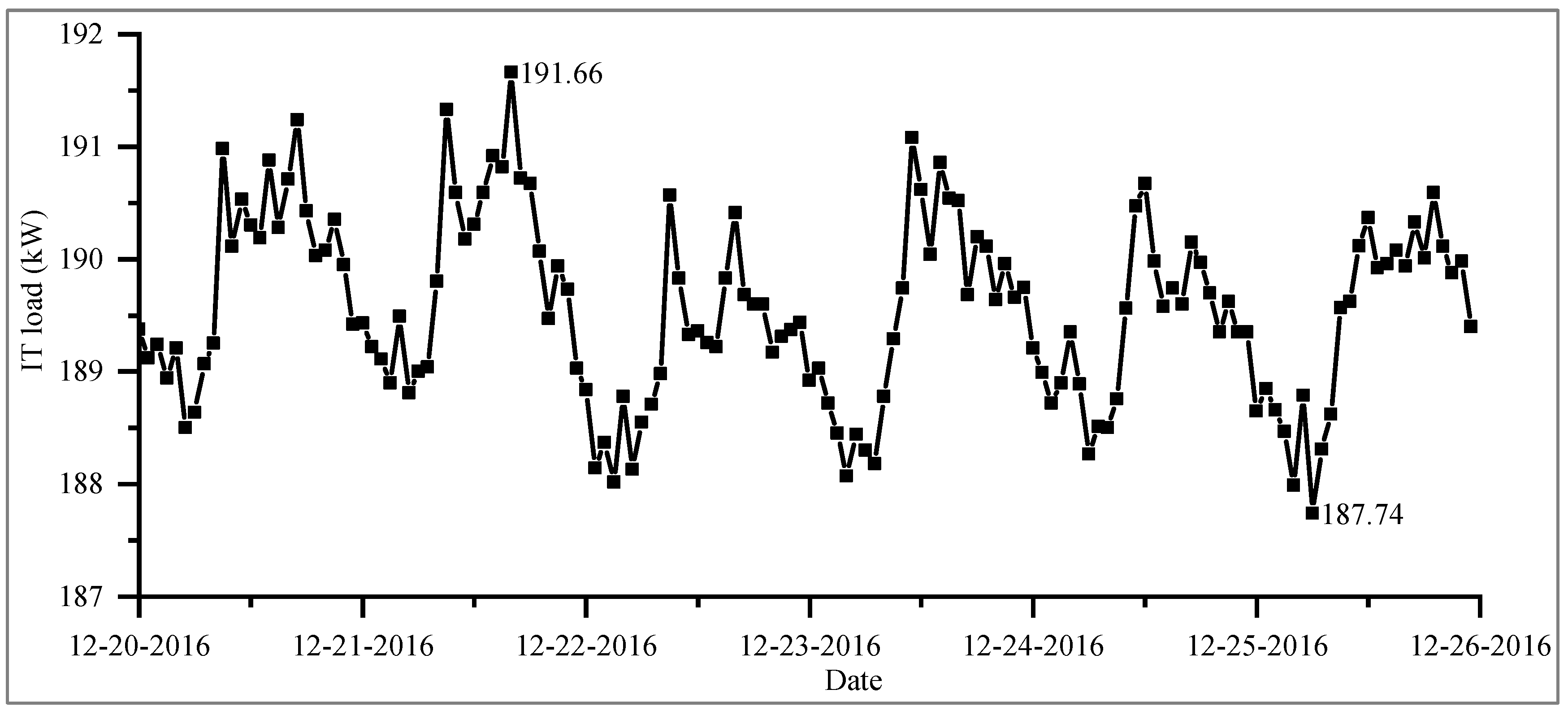
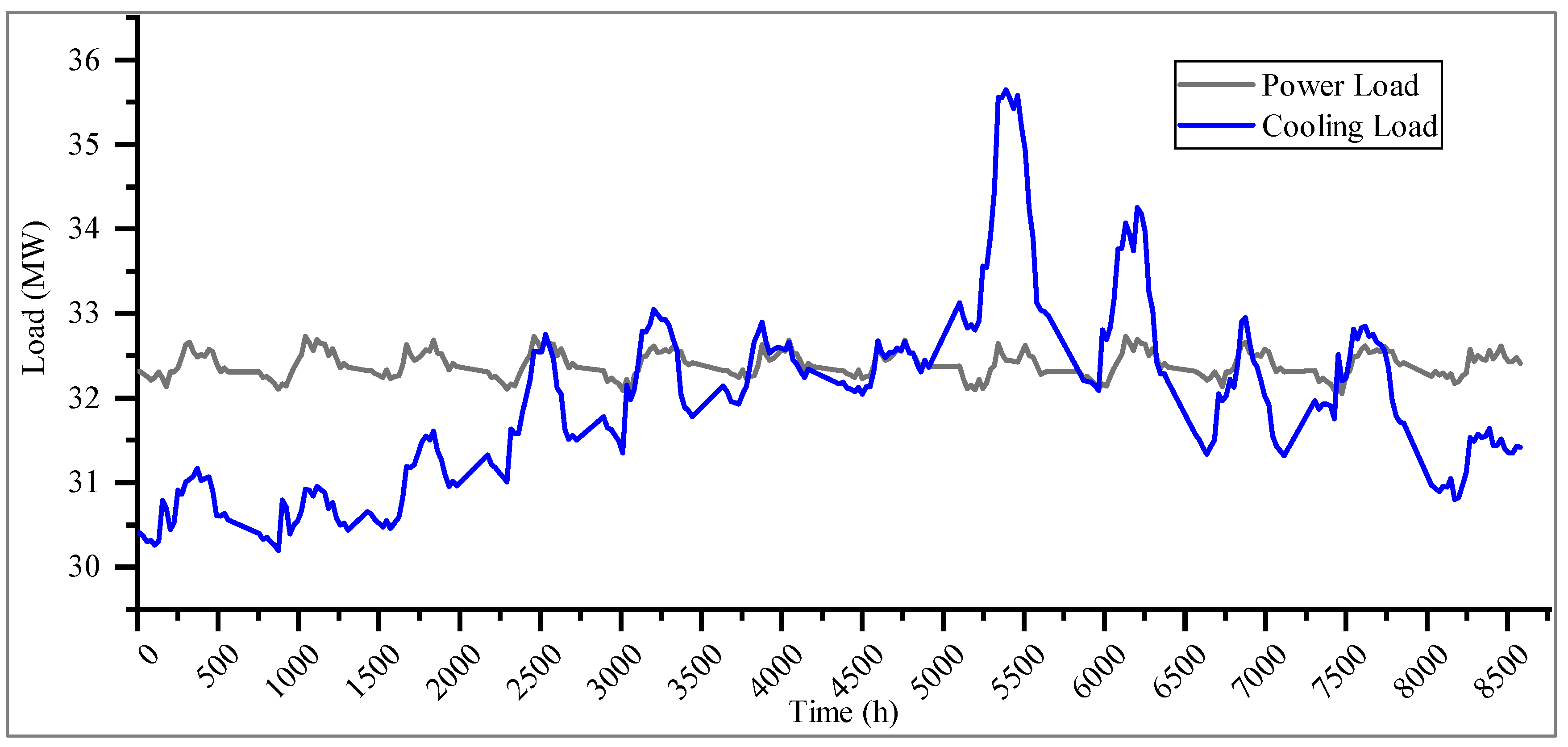
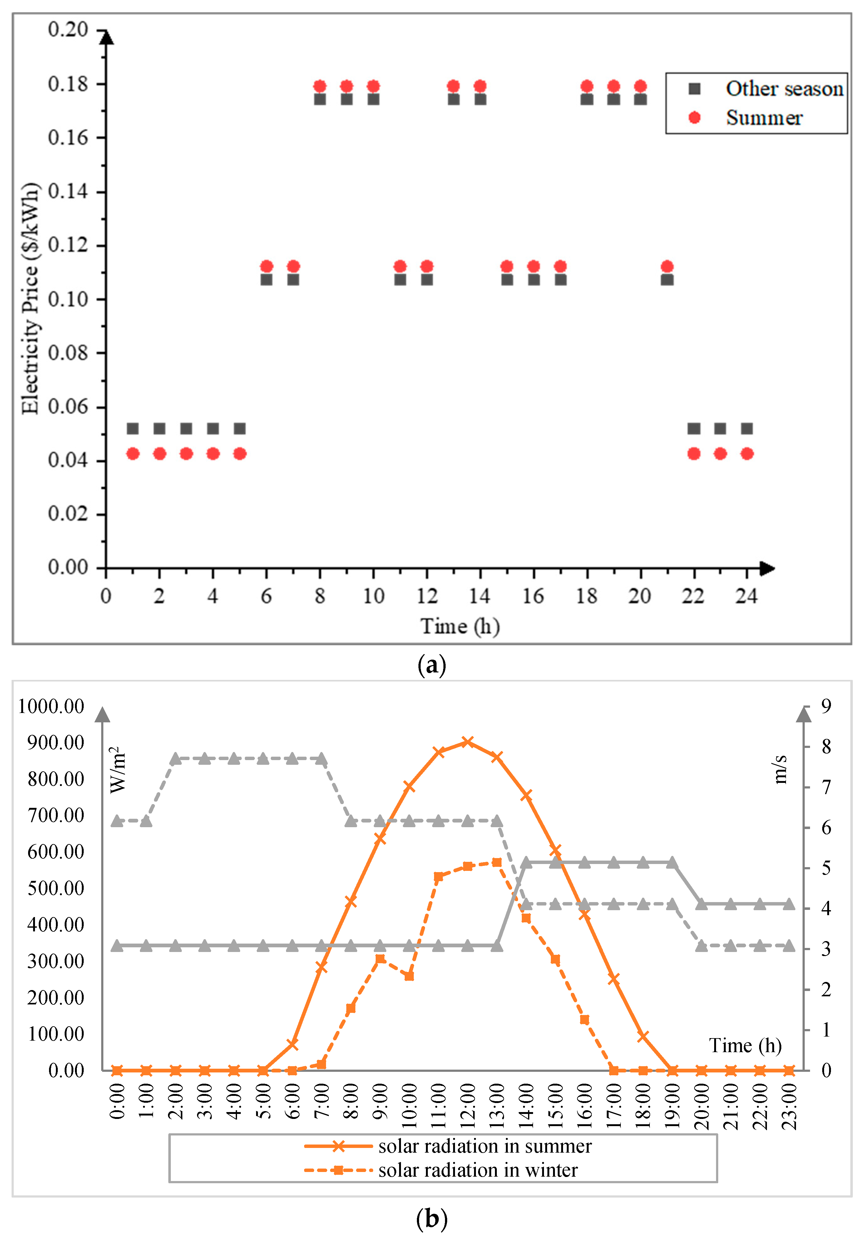
4.1. Cooling and Power Load Prediction Using Operational Data

In this study, a real data center park (DCP) located in Shanghai, China was selected as a case study to implement the configuration method developed in this study. Hourly power consumption data of IT equipment were collected during the period of 19 December and 25 December 2016 by monitoring the active power output of the UPS, as shown in Figure 5. These data were then put into Energy Plus [39,40], a popular dynamic building performance simulation engine, to calculate the hourly power load and cooling load of this DCP, with results shown in Figure 6. Apparently, the cooling load in winter was less than the electrical load, owing to the heat loss through the building fabric, whereas in summer, the opposite behavior took place.

4.2. Basic Parameter Determination

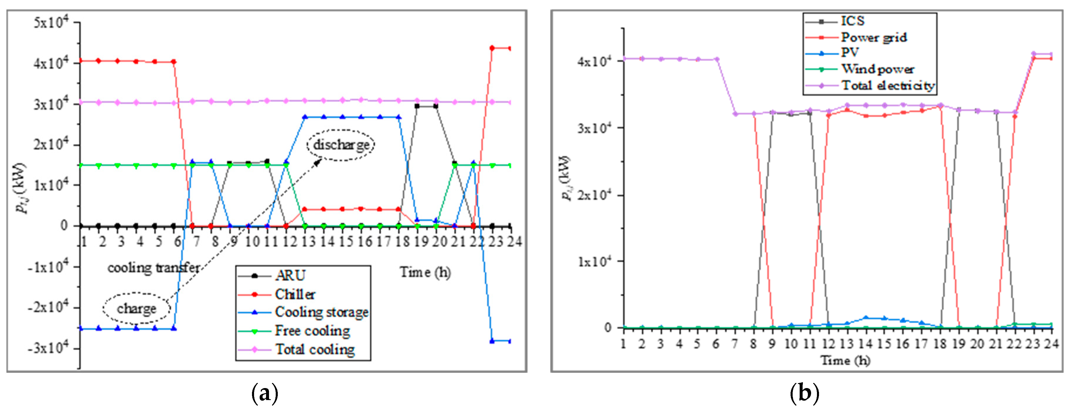
For the configuration model developed in this study, its basic input parameters include the cooling and electrical loads, natural gas price, electricity price, local renewable energy resources, equipment performance parameters, and equipment price parameters. The time-of-use electricity price, wind, and solar resources are illustrated in Figure 7. Equipment parameters and others are listed in

Table 3. Input parameters for equipment.

Device J	$\mathit{P}\mathit{r} (\mathbf{\$}/\mathbf{kW})$	$\mathit{\alpha } (\mathbf{\$}/\mathbf{kW})$	$\mathit{\beta } (\mathbf{\$}/\mathbf{kWh})$	$\mathit{n} \left(\mathbf{Years}\right)$	$\mathit{P}{\mathit{r}}_{\mathit{g}} (\mathbf{\$}/{\mathbf{m}}^3)$	${\mathit{\eta }}_{\mathit{e}} (\%)$	COP
1	225.03	1.93	0.014	20	0.46	40	-
2	99.82	1.77	0.004	15	-	-	0.9
3	74.72	1.77	0.003	20	-	-	5.8
4	16.83	1.40	0.003	20	-	-	-
5	114.08 $/m3	1.57	0.003	20	-	-	-
6	14.26	0.00	0.003	20	-	-	-
7	798.59	2.07	0.013	25	-	-	-
8	926.93	2.07	0.013	20	-	-	-

.

4.3. Results

The DCP-IES configuration model developed in this study is a MILP model, and Cplex in GAMS was selected as the tool for solving the calculations. In the MILP model, there are not only continuous variables but also integer variables, and there are two methods to solve the MILP problem, namely the Branch and Bound method and Cutting Plane method. The Branch-and-Cut Algorithm (BCA) adopted in the study is a combination of the above two methods. BCA is a typical classic optimization algorithm for solving MILP problems. It can be solved by calling a commercial solver. The global optimal and unique solution can be obtained by using BCA, but it requires more computing time. In addition, the MILP problem is generally non-deterministic polynomial hard problem, and the algorithm of MILP problem is generally non polynomial complexity algorithm. The computational complexity belongs to type $O\left(a^n\right)$, where $a$ is a constant, $n$ is the number of variables. In other words, when choosing the classic optimization algorithm to solve the configuration model established in the paper, the number of variables should be within a certain limit, otherwise the result will not converge. Therefore, only the typical daily energy configuration is calculated in the paper. On the other hand, the currently popular metaheuristic optimization algorithms have strong generalized solving ability, which can be used to solve the MILP problem. However, the optimal solutions of metaheuristic algorithms are usually not the global optimal. To this end, the computing time and optimal results between the BCA and NSGA-II are compared, as shown in

Table 4. Computing time and optimal results of BCA and NSGA-II.

Iterations		1	20	40	60	80	100	120	140
Computing time (s)	BCA	1803	1743	1821	1845	1794	1827	1819	1807
	NSGA-II	150	167	334	497	733	1972	2145	3156
INI 1 (million USD)	BCA	35.09	35.09	35.09	35.09	35.09	35.09	35.09	35.09
	NSGA-II	37.69	36.69	35.86	36.36	35.19	35.69	35.36	35.16
OC 2 (million USD)	BCA	30.45	30.45	30.45	30.45	30.45	30.45	30.45	30.45
	NSGA-II	32.17	31.99	32.06	31.09	30.74	31.16	31.31	30.81
CE 3 (tCO2)	BCA	232,250	232,250	232,250	232,250	232,250	232,250	232,250	232,250
	NSGA-II	245,335	243,972	244,517	237,157	234,431	237,702	238,792	234,976

¹ INI—Initial investment; ² OC—Operating cost; ³ CE—Carbon emissions.

. The population size of the NSGA-II is set to 50–200, and the genetic algebra is set to 500. From Table 4, the more the iteration is, the longer the computing time of NSGA-II is. However, as the iteration increases, the computing time of BCA remains the same basically. Moreover, the optimal results of NSGA-II are worse than that of BCA. Therefore, BCA is selected as the solution algorithm of MILP model with acceptable computing time and stable optimal results.

The calculation results were compared with those calculated from a traditional data center energy system (TDC-ES), which is powered by a power grid and cooled by chillers. The cost and carbon emissions for both the DCP-IES and TDC-ES are shown in

Table 5. Cost and carbon emissions for both DCP-IES and TDC-ES.

Types	CCP	AC 1	Chiller	FC 2	CS 3	PG 4	PV	WP 5	Total
DCP-IES INI (million USD)	7.37	2.94	5.18	0.26	3.81	9.57	4.88	1.10	35.09
DCP-IES OC (million USD)	10.27	0.33	0.64	0.11	0.56	18.42	0.10	0.01	30.45
DCP-IES CE (tCO2)	42,488	0	0	0	0	189,762	0	0	232,250
TDC-ES INI (million USD)	0	0	2.99	0	0	8.71	0	0	11.71
TDC-ES OC (million USD)	0	0	0.86	0	0	37.69	0	0	38.55
TDC-ES CE (tCO2)	0	0	0	0	0	271,573	0	0	271,573

¹ AC—Absorption chiller; ² FC—Free-cooling; ³ CS—Cooling storage; ⁴ PG—Power grid; ⁵ WP—Wind power.

. It is worth noting that the initial investment (INI) in Table 5 does not include the INI of the redundant equipment. From Table 5, the INI of the DCP-IES was $23.38 million higher than that for TDC-ES; however, the annual operational cost (OC) was $8.10 million lower. It will only take 2.88 years for the economics of DCP-IES to reach those of TDC-ES. Afterwards, the economics of DCP-IES will be better than those of TDC-ES. The investment payback period (PP) of TDC-ES and DCP-IES also are calculated, respectively, according to the annual income and initial cost, as shown in Equation (27), where $C_{in}$ is the initial cost; $C_o$ is the annual operative cost; $S{P}_e$ and $S{P}_c$ are the selling price of electricity and cooling, respectively; $L{E}_t$ and $L{C}_t$ represent the electrical load and cooling load at time $t$. Generally, the investment payback period varies with the selling price of cooling and electricity. Therefore, let $S{P}_e=0.114$ USD/kWh and $S{P}_c=0.083$ USD/kWh in this paper based on engineering experience. The investment payback period of DCP-IES and TDC-ES are 3.41 and 6.59 years respectively, which can be calculated by Equation (27). In addition, the carbon emissions (CE) of DCP-IES were 39,323 tons lower than those of TDC-ES. Based on Equation (1) and the obtained operational strategy, the PUE of DCP-IES is 1.389. In summary, the energy allocation using the configuration model is better than that of the traditional energy system, although its initial investment is higher.

$$PP=\frac{C_{in}}{{{\displaystyle \sum }}_{t=1}^{8760}\left(S{P}_{e}L{E}_t+S{P}_{c}L{C}_t\right)-C_o},$$

(27)

Based on the results from the configuration model, hourly outputs of eight energy conversion technologies were obtained for the entire year. The operation strategies of cooling and electricity in a typical winter day and typical summer day are illustrated in Figure 8 and Figure 9, respectively. The outputs for both PV and wind power were small, owing to the availability of natural resources. Influenced by the fluctuations of the electrical price in the power grid, the electricity was served by either the CCP or the power grid at different times during the day. This type of alternating output leads to frequent switching of the multi-energy complementary system. In actual operation, the device, especially the absorption chiller, has a pre-starting time, which cannot realize real-time switching. Therefore, before applying the configuration model established in this study, it is necessary to design the relevant switching logic and analyze the possible system faults caused by the device switching. Then, the relevant constraints to avoid those faults are fed back into the configuration model to repair and improve the model. The next section demonstrates the analysis of this problem.

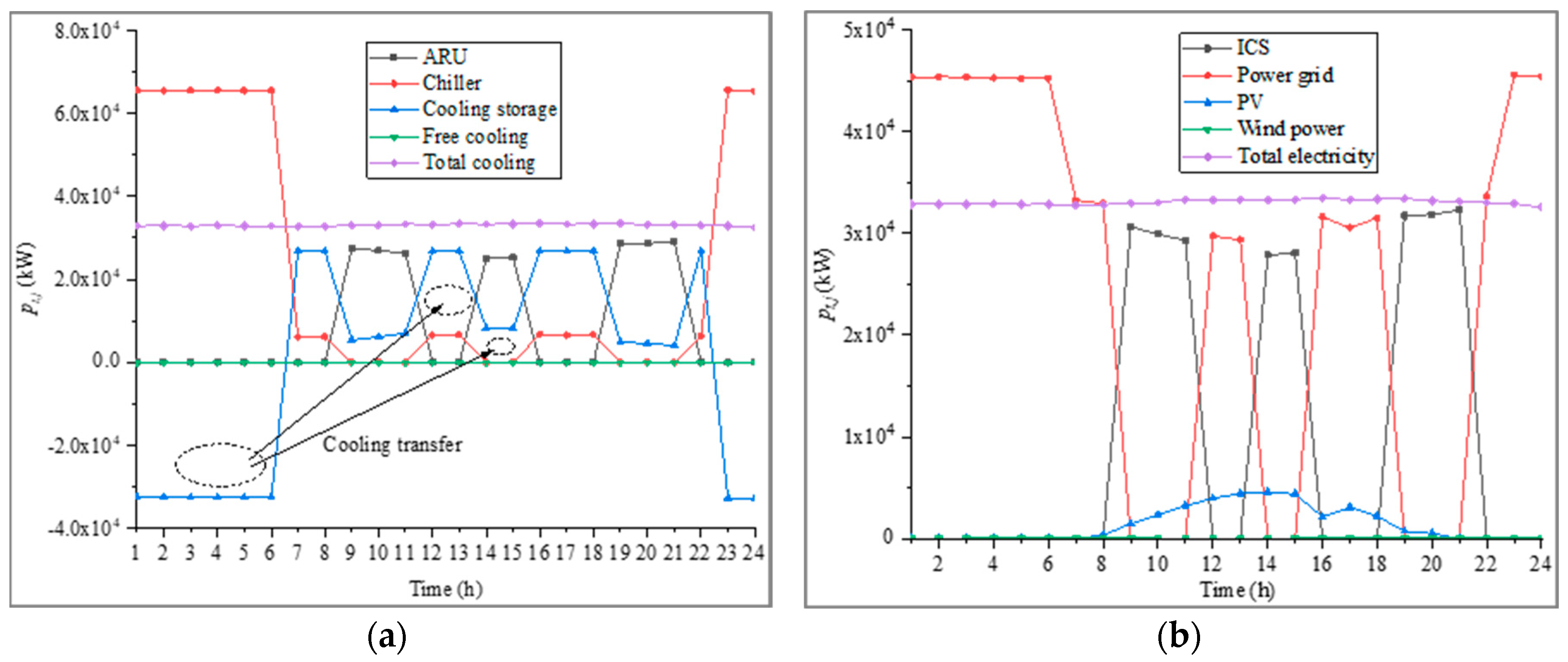
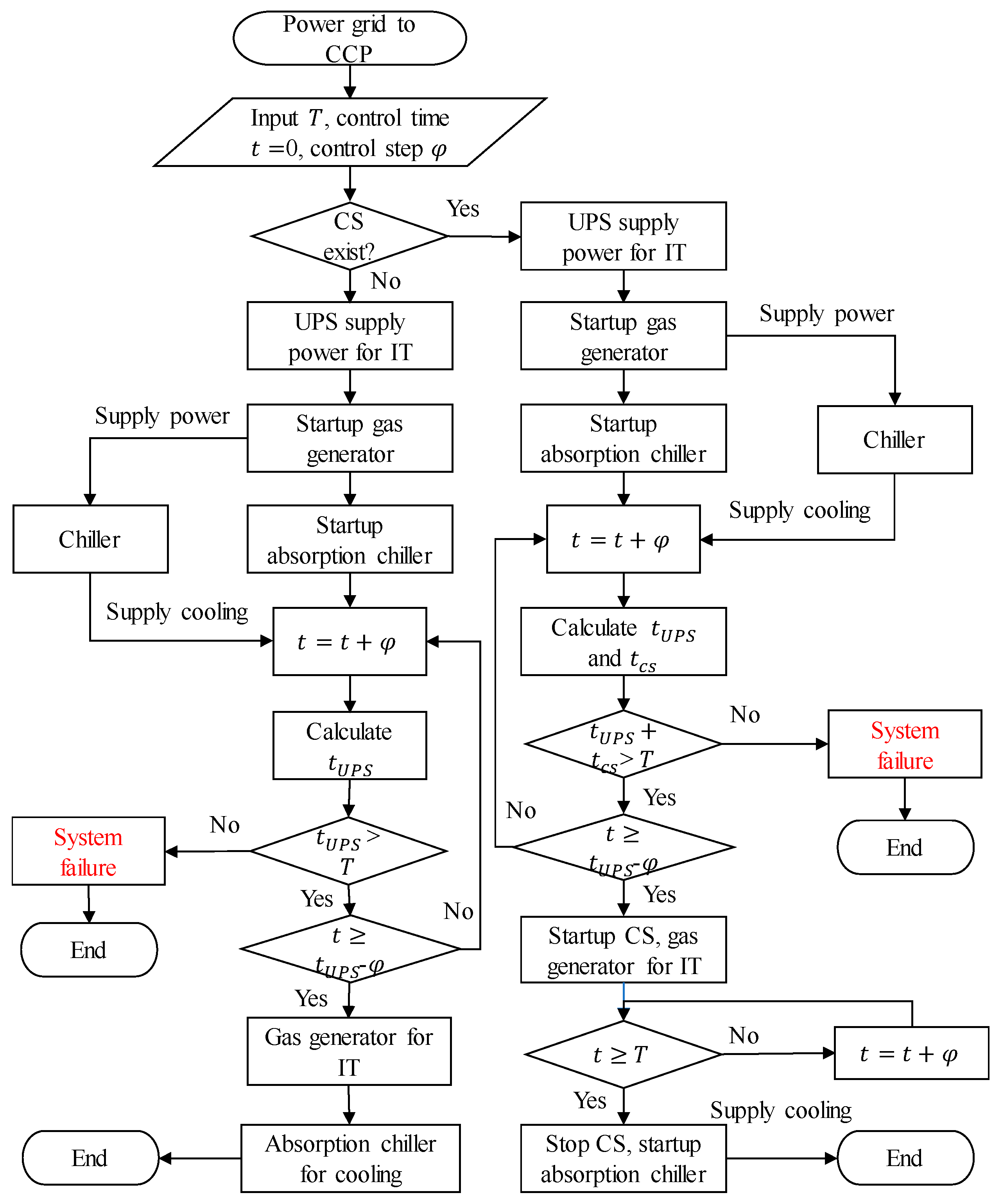
4.4. Switching Logic Analysis

A simplified diagram for the DCP-IES is provided in Figure 10. According to the optimal configuration results, the switching logic between a large power grid and CCP is given, as shown in Figure 11.

From Figure 11, when switching from a large grid power to CCP, the system determines whether cooling storage is available. If cooling storage is available, the following instructions are executed: calculate the cooling storage continuous working time ($t_{cs}$), and calculate the UPS storage capacity ($C{a}_{UPS}$) and continuous working time ($t_{UPS}$). From this operation, the start-up sequence and number of devices needed are determined. The pre-cooling time for the absorption chiller was set as $T=40$ min. As can be seen from Figure 11, there are two system failures that cannot guarantee the normal operation of DCP-IESs, which are caused by the relationship among $t_{UPS}$, $t_{cs}$, and $T$. Parameters $t_{UPS}$ and $t_{cs}$ are calculated by Equations (28) and (29), respectively. Therefore, the two following constraints could be used to ensure the reliability of switching: First, the configuration capacity of CCP is increased to provide sufficient power for the IT equipment and chillers during the pre-cooling time of the absorption chillers, as shown in Equation (30), and second, the configuration capacities of the UPS and cooling storage are increased, as shown in Equation (31).

$${{\displaystyle \sum }}_{t=1}^{t_{cs}}\left(L{C}_t-p_{t,3}-p_{t,4}\right)=C{a}_{cs},$$

(28)

$${{\displaystyle \sum }}_{t=1}^{t_{UPS}}\left(L{E}_{t,IT}+L{E}_{t,chiller}-p_{t,1}\right)=C{a}_{UPS},$$

(29)

where $C{a}_{cs}$ is the available capacity of cooling storage in kWh, $C{a}_{UPS}$ is the available capacity of UPS in kWh, $L{C}_t$ is the cooling load of DCP-IES at time t in kW, $L{E}_{t,IT}$ and $L{E}_{t,chiller}$ are the electricity load of IT and chiller at time $t$ in kW, respectively, and $p_{t,1}$, $p_{t,3}$, and $p_{t,4}$ are the outputs of device $j$ at time $t$, $j=1, 3, 4$, respectively.

$$p_{t,1}\ge \frac{p_{t,2}}{CO{P}_3}+L{E}_t,t\le T,$$

(30)

$$t_{cs}+t_{UPS}\ge T,$$

(31)

where $CO{P}_3$ is the efficiency of the chiller, $L{E}_t$ is the total electricity load of the DCP-IES at time $t$, including IT, chiller, etc. Equations (30) and (31) can be brought into the configuration model as a constraint to avoid switching faults. Clearly, the above switching logic is based on the fact that the chillers can meet the total cooling load solely. The optimal configuration results (Table 5) indicate that the optimization results satisfy the condition. In summary, a multi-objective configuration optimization model that considers the device pre-start time is established.

4.5. Reliability Analysis and Redundant Design

After obtaining the optimal energy configuration based on cost, carbon emissions, and device pre-start, as shown in

Table 6. Modified optimization energy configuration of DCP-IES.

Devices	Capacity (kW)	Quantity	INI (Million USD)	OC (Million USD)
CCP	8500	4	7.57	10.27
AC	7624	4	2.94	0.33
Chiller	2800USRT 1	7	5.21	0.67
FC	2500	6	0.26	0.11
CS	10,000 m3	2	3.82	0.56
PG	46,276	1	9.57	18.42
PV	6100	-	4.88	0.10
WP	1186	-	1.10	0.01
Total	-	-	35.34	30.63

¹ 1 USRT = 3.517 kW.

, the energy system needs to be designed redundantly and evaluated for reliability. When the equipment fails, the standby equipment can be used to ensure the normal operation of the DCP-IES; this is the redundant design. Then, the reliability analysis of DCP-IES is carried out by using the reliability estimation method in Section 3.4. In the redundant design of DCP-IESs, the reliability of the system could be improved by increasing the number of standby devices. However, this would result in an increased INI. In particular, for an increase in the reliability of the energy supply by a certain amount, a small increase in reliability would require a huge financial cost. Therefore, the reliability analysis of the DCP-IES must be accompanied by a cost calculation to obtain the optimal redundant design.

Comparing Table 5 and Table 6 shows that the configuration capacity of CCP was larger than the result before correction, and the total INI increased by $0.24 million with a PUE of 1.388. When redundant design is performed on the above configuration results, it does not affect the OC of the DCP-IES. Therefore, the economic analysis of redundant design can be simplified to the INI analysis. Furthermore, 12 redundant scenarios were established to analysis the reliability and INI of the DCP-IES, as shown in Figure 12, where Scenario A was no redundant design, Scenario B was power grid redundancy, and Scenario C was diesel-generator redundancy.

The failure rate and repair rate of each device required in Section 3.4 are shown in

Table 7. Failure rate and repair rate of each device [38].

Device	CCP	AC	Chiller	FC	CS	PG	PV	WP
Failure rate (time/day)	0.00547945	0.00136986	0.000913240	0.000684790	0.0103903	0.00305800	0.0170452	0.0121137
Repair rate (time/day)	2.541667	2.000000	2.000000	1.000000	1.000000	5.083333	3.2906082	3.4042571

. Using the reliability estimation method in Section 3.4 and topological structure shown in Figure 10, the available rate of electricity, available rate of cooling, and INI in all 12 redundant scenarios could be obtained, as shown in

Table 8. Reliability and initial investment of DCP-IES for all 12 redundant scenarios.

Redundant Scenario	Available Rate of Electricity (%)	Available Rate of Cooling (%)	INI (Million USD)
A	99.9399	99.9894	35.34
A1	99.9900	99.9897	37.11
A2	99.9399	99.9940	35.64
A3	99.9900	99.9948	37.41
B	99.9996	99.9954	44.91
B1	99.9998	99.9957	46.67
B2	99.9996	99.9992	45.21
B3	99.9998	99.9993	46.97
C	99.9989	99.9935	43.44
C1	99.9995	99.9935	45.21
C2	99.9989	99.9989	43.74
C3	99.9995	99.9990	45.51

. It should be noted that the presence of a standby CCP or standby chiller signifies that only one more CCP or chiller is reserved. If two CCPs or chillers were to fail during the operation, the system would malfunction.

Table 8 shows that the minimum INI was $35.34 million for no standby device, as defined in Scenario A. Not surprisingly, the energy supply reliability was the lowest, with the available rates of electricity and cooling of 99.9399% and 99.9894%, respectively. The electricity supply reliability in Scenarios B1 and B3 was 99.9998%, which was the highest for all scenarios, and the corresponding INIs were $46.67 and $46.97 million, respectively. The cooling available rate of Scenario B3 was the highest among all, with the available rate of cooling and INI of 99.9993% and $46.97 million, respectively. To meet the five “9” reliability requirements of electricity and cooling supply in the DCP-IES design, the redundant design of Scenario B2 was concluded to be the most appropriate, with the INI of $45.21 million. Additionally, as shown in Table 8, when the reliability changed from the three “9” in Scenario A to the four “9” in Scenario A3 and to the five “9” in Scenario B2, the INI increased from $35.34 million to $37.41 million and then to $45.21 million, i.e., as the reliability increases, the INI increases increasingly faster. In summary, the DCP-IES configuration method was obtained under the comprehensive considerations of cost, carbon emissions, device pre-start, and reliability.

5. Conclusions

With the rapid development of information technology, integrated data centers, mostly in the basic form of parks, were built extensively. These buildings are often characterized as high energy intensive with stable load and high carbon emissions, which is very beneficial to the integrated use of multiple sources of energy in the DCP. In this context, the economical and low-carbon multi-objective configuration model was established based on the MILP method, and the configuration model was modified according to the security of the device switching. Then, the configuration results were designed redundantly using the reliability estimation method based on Markov processes. Finally, the DCP-IES configuration method was obtained under the comprehensive considerations of cost, carbon emissions, device pre-start, and reliability. The following conclusions were drawn:

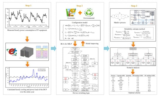
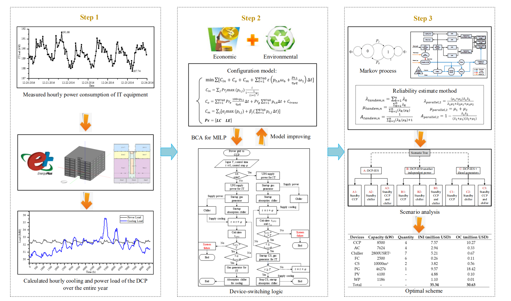
• In the multi-objective configuration model, the carbon emissions of DCP-IESs were converted into economic indicators through carbon pricing and were optimized for the initial investment, operational costs, and maintenance costs of the system. Renewable energy, waste heat, free-cooling, and cooling storage were all considered. Compared with traditional energy systems, the results indicated that it would only take 2.88 years for the economics of the DCP-IES to catch up to those of the TDC-ES; the carbon emissions of the DCP-IES were 39,323 tons lower than those for the TDC-ES, and the PUE was 1.389.
• Multi-energy integration led to the frequent device switching of the DCP-IES. Based on the given device switching logic, the relevant constraints for avoiding the switching faults were fed back into the configuration model to correct the model. The results indicated that the total initial investment increased by $0.24 million, and the PUE was 1.388.
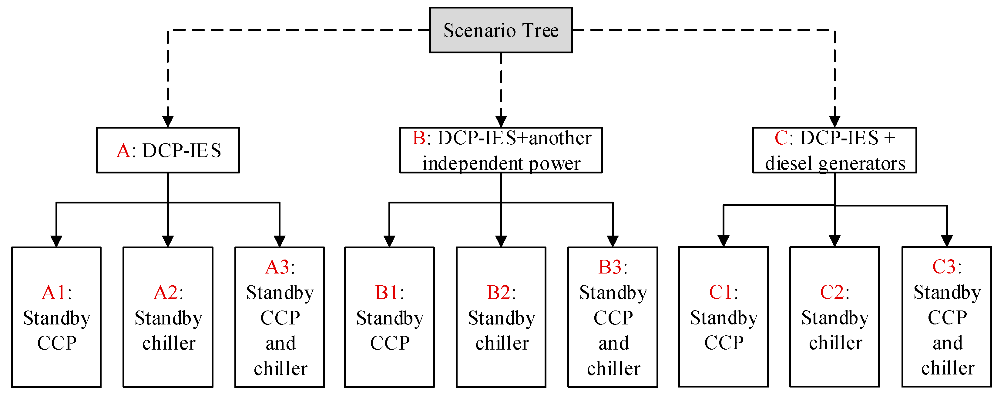
• In 12 scenarios of redundant design, both the cooling availability and power availability of DCP-IESs were calculated for systems with parallel- and series-arranged devices, based on Markov processes. The results indicated that the total initial investment for the DCP-IES meeting the four “9” reliability requirement, represented by Scenario A3, was $37.41 million, and the total initial investment for the DCP-IES meeting the five “9” reliability requirement, represented by Scenario B2, was $45.21 million. As the reliability increases, the initial investment cost increases increasingly faster.
• Using the new energy configuration method, the configuration scheme of the DCP-IES could be obtained under economical, low-carbon, and reliability requirements. With the help of the new DCP-IES configuration model, DCP planners can easily obtain energy indicators during the planning stage, designers can quickly achieve low-carbon energy allocations, and operators can obtain operational strategies of system devices based on real-time load forecasting results.

However, there are still some limitations. The step size of the dispatch with regard to cooling and electricity is one hour in the paper under the complexity considerations of energy system configuration process. Therefore, the configuration model cannot achieve the cooling and electricity joint optimal configuration in one minute. The solution complexity of the configuration model grows exponentially with the increase of variables. Hence, it is difficult to use the model to solve the hourly equipment configuration over an entire year, when there are a large number of available devices. The operational efficiency of each device will vary with the operational conditions in actual engineering applications. However, only chillers were considered in this study. Additionally, any surplus electricity generated in the DCP-IES should be delivered to the power grid. These issues will be considered in future research.

References

1. China National Information Infrastructure. The Research Report of Chinese IDC Market Trend and Investment Strategy in 2017–2019; China National Information Infrastructure: Beijing, China, 2016. [Google Scholar]
2. Song, X.; Liu, L.; Zhu, T.; Zhang, T.; Wu, Z. Comparative analysis on operation strategies of CCHP system with cool thermal storage for a data center. Appl. Therm. Eng. 2016, 108, 680–688. [Google Scholar] [CrossRef]
3. Huang, P.; Copertaro, B.; Zhang, X.; Shen, J.; Löfgren, I.; Rönnelid, M.; Fahlen, J.; Andersson, D.; Svanfeldt, M. A review of data centers as prosumers in district energy systems: Renewable energy integration and waste heat reuse for district heating. Appl. Energy 2020, 258, 114109. [Google Scholar] [CrossRef]
4. Rong, H.; Zhang, H.; Xiao, S.; Li, C.; Hu, C. Optimizing energy consumption for data centers. Renew. Sustain. Energy Rev. 2016, 58, 674–691. [Google Scholar] [CrossRef]
5. Ding, T.; He, Z.G.; Hao, T.; Li, Z. Application of separated heat pipe system in data center cooling. Appl. Therm. Eng. 2016, 109, 207–216. [Google Scholar] [CrossRef]
6. Jaureguialzo, E. PUE: The Green Grid metric for evaluating the energy efficiency in DC (Data Center). Measurement method using the power demand. In Proceedings of the 2011 IEEE 33rd International Telecommunications Energy Conference (INTELEC), Amsterdam, The Netherlands, 9–13 October 2011; pp. 1–8. [Google Scholar]
7. Sharma, M.; Arunachalam, K.; Sharma, D. Analyzing the data center efficiency by using PUE to make data centers more energy efficient by reducing the electrical consumption and exploring new strategies. Procedia Comput. Sci. 2015, 48, 142–148. [Google Scholar] [CrossRef] [Green Version]
8. International Energy Agency. Global Energy & CO2 Status Report; International Energy Agency: Paris, France, 2018. [Google Scholar]
9. Sevencan, S.; Lindbergh, G.; Lagergren, C.; Alvfors, P. Economic feasibility study of a fuel cell-based combined cooling, heating and power system for a data centre. Energy Build. 2016, 111, 218–223. [Google Scholar] [CrossRef] [Green Version]
10. Rossi, F.D.; Xavier, M.G.; De Rose, C.A.F.; Calheiros, R.N.; Buyya, R. E-eco: Performance-aware energy-efficient cloud data center orchestration. J. Netw. Comput. Appl. 2017, 78, 83–96. [Google Scholar] [CrossRef]
11. Asghari, N.; Mandjes, M.; Walid, A. Energy-efficient scheduling in multi-core servers. Comput. Netw. 2014, 59, 33–43. [Google Scholar] [CrossRef]
12. Li, X.; Qian, Z.; Lu, S.; Wu, J. Energy efficient virtual machine placement algorithm with balanced and improved resource utilization in a data center. Math. Comput. Model. 2013, 58, 22–35. [Google Scholar] [CrossRef]
13. Wang, Y.; Wang, X. Performance-controlled server consolidation for virtualized data centers with multi-tier applications. Sustain. Comput. Inform. Syst. 2014, 4, 52–65. [Google Scholar] [CrossRef]
14. Chen, H.; Zhu, X.; Guo, H.; Qin, X.; Zhu, J.; Wu, J. Towards energy-efficient scheduling for real-time tasks under uncertain cloud computing environment. J. Syst. Softw. 2014, 53, 50–58. [Google Scholar] [CrossRef]
15. Cho, K.; Chang, H.; Jung, Y.; Yoon, Y. Economic analysis of data center cooling strategies. Sustain. Cities Soc. 2017, 31, 234–243. [Google Scholar] [CrossRef]
16. Ni, J.; Bai, X. A review of air conditioning energy performance in data centers. Renew. Sustain. Energy Rev. 2017, 67, 625–640. [Google Scholar] [CrossRef]
17. Lu, H.; Zhang, Z.; Yang, L. A review on airflow distribution and management in data center. Energy Build. 2018, 179, 264–277. [Google Scholar] [CrossRef]
18. Ham, S.-W.; Kim, M.-H.; Choi, B.-N.; Jeong, J.-W. Energy saving potential of various air-side economizers in a modular data center. Appl. Energy 2015, 138, 258–275. [Google Scholar] [CrossRef]
19. Yu, J.; Jiang, Y.; Yan, Y. A simulation study on heat recovery of data center: A case study in Harbin, China. Renew. Energy 2019, 130, 154–173. [Google Scholar] [CrossRef]
20. Oró, E.; Depoorter, V.; Garcia, A.; Salom, J. Energy efficiency and renewable energy integration in data centres. Strategies and modelling review. Renew. Sustain. Energy Rev. 2015, 42, 429–445. [Google Scholar] [CrossRef]
21. Tian, H.; He, Z.; Li, Z. A combined cooling solution for high heat density data centers using multi-stage heat pipe loops. Energy Build. 2015, 94, 177–188. [Google Scholar] [CrossRef]
22. Yue, C.; Zhang, Q.; Zhai, Z.; Ling, L. Numerical investigation on thermal characteristics and flow distribution of a parallel micro-channel separate heat pipe in data center. Int. J. Refrig. 2019, 98, 150–160. [Google Scholar] [CrossRef]
23. Zhou, F.; Wei, C.; Ma, G. Development and analysis of a pump-driven loop heat pipe unit for cooling a small data center. Appl. Therm. Eng. 2017, 124, 1169–1175. [Google Scholar] [CrossRef]
24. Dong, K.; Li, P.; Huang, Z.; Su, L.; Sun, Q. Research on free cooling of data centers by using indirect cooling of open cooling tower. Procedia Eng. 2017, 205, 2831–2838. [Google Scholar] [CrossRef]
25. Yang, Y.; Wang, B.; Zhou, Q. Air conditioning system design using free cooling technology and running mode of a data center in Jinan. Procedia Eng. 2017, 205, 3545–3549. [Google Scholar] [CrossRef]
26. Zhang, H.; Shao, S.; Xu, H.; Zou, H.; Tian, C. Free cooling of data centers: A review. Renew. Sustain. Energy Rev. 2014, 35, 171–182. [Google Scholar] [CrossRef]
27. Sheme, E.; Holmbacka, S.; Lafond, S.; Lučanin, D.; Frashëri, N. Feasibility of using renewable energy to supply data centers in 60° north latitude. Sustain. Comput. Inform. Syst. 2018, 17, 96–106. [Google Scholar] [CrossRef]
28. Wang, Y.; Wang, X.; Yu, H.; Huang, Y.; Dong, H.; Qi, C.; Baptiste, N. Optimal design of integrated energy system considering economics, autonomy and carbon emissions. J. Clean. Prod. 2019, 225, 563–578. [Google Scholar] [CrossRef]
29. Tran, H.N.; Narikiyo, T.; Kawanishi, M.; Kikuchi, S.; Takaba, S. Whole-day optimal operation of multiple combined heat and power systems by alternating direction method of multipliers and consensus theory. Energy Convers. Manag. 2018, 174, 475–488. [Google Scholar] [CrossRef]
30. Van der, H.; Vandermeulen, A.; Salenbien, H. Integrated optimal design and control of fourth generation district heating networks with thermal energy storage. Energies 2019, 12, 2766. [Google Scholar] [CrossRef] [Green Version]
31. Reynolds, J.; Ahmad, M.W.; Rezgui, Y.; Hippolyte, J.-L. Operational supply and demand optimisation of a multi-vector district energy system using artificial neural networks and a genetic algorithm. Appl. Energy 2019, 235, 699–713. [Google Scholar] [CrossRef]
32. Ritchie, A.J.; Brouwer, J. Design of fuel cell powered data centers for sufficient reliability and availability. J. Power Sources 2018, 384, 196–206. [Google Scholar] [CrossRef]
33. Wang, J.; Zhang, Q.; Yoon, S.; Yu, Y. Reliability and availability analysis of a hybrid cooling system with water-side economizer in data center. Build. Environ. 2019, 148, 405–416. [Google Scholar] [CrossRef]
34. Figueirêdo, J.; Maciel, P.; Callou, G.; Tavares, E.; Sousa, E.; Silva, B. Estimating reliability importance and total cost of acquisition for data center power infrastructures. In Proceedings of the 2011 IEEE International Conference on Systems, Man, and Cybernetics, Anchorage, AK, USA, 9–12 October 2011; pp. 421–426. [Google Scholar]
35. Ma, H.; Li, C.; Lu, W.; Zhang, Z.; Yu, S.; Du, N. Experimental study of a multi-energy complementary heating system based on a solar-groundwater heat pump unit. Appl. Therm. Eng. 2016, 109, 718–726. [Google Scholar] [CrossRef]
36. Gillespie, D.T. (Ed.) 1-RANDOM VARIABLE THEORY. In Markov Processes; Academic Press: San Diego, CA, USA, 1992; pp. 1–58. [Google Scholar]
37. Cranston, M.; Greven, A. Coupling and harmonic functions in the case of continuous time Markov processes. Process. Their Appl. 1995, 60, 261–286. [Google Scholar] [CrossRef] [Green Version]
38. Wang, J. Optimal Design of Building Cooling Heating and Power System and Its Multi-Criteria Integrated Evaluation Method; North China Electric Power University: Beijing, China, 2012. [Google Scholar]
39. Crawley, D.B.; Lawrie, L.K.; Winkelmann, F.C.; Buhl, W.F.; Huang, Y.J.; Pedersen, C.O.; Strand Richard, K.; Liesen Richard, J.; Fisher Daniel, E.; Witte Michael, J.; et al. EnergyPlus: Creating a new-generation building energy simulation program. Energy Build. 2001, 33, 319–331. [Google Scholar] [CrossRef]
40. Fumo, N.; Mago, P.; Luck, R. Methodology to estimate building energy consumption using Energy Plus Benchmark Models. Energy Build. 2010, 42, 2331–2337. [Google Scholar] [CrossRef]
Figure 1. The market size of IDCs in China and the world.
Energies 13 00448 g001
Figure 2. (a) Energy consumption structure of typical IDC in China; (b) Energy consumption structure of typical IDC in the world.
Energies 13 00448 g002
Figure 3. Logical structure of the paper.
Energies 13 00448 g003
Figure 4. The three coupled configuration issues in DCP-IES.
Energies 13 00448 g004
Figure 5. Measured hourly power consumption of IT equipment.
Energies 13 00448 g005
Figure 6. Calculated hourly cooling and power load of the DCP over the entire year.
Energies 13 00448 g006
Figure 7. (a) Time-of-use electricity price in Shanghai; (b) Renewable energy in a typical day in Shanghai.
Energies 13 00448 g007
Figure 8. (a) Operational strategies of cooling equipment in a typical winter day; (b) Operational strategies of power generation equipment in a typical winter day.
Energies 13 00448 g008
Figure 9. (a) Operational strategies of cooling equipment in a typical summer day; (b) Operational strategies of power generation equipment in a typical summer day.
Energies 13 00448 g009
Figure 10. Simplified diagram for energy supply systems.
Energies 13 00448 g010
Figure 11. Switching logic of DCP-IES.
Energies 13 00448 g011
Figure 12. Scenario tree of redundant design for DCP-IES.
Energies 13 00448 g012