Article

Carbon and Water Footprint of Energy Saving Options for the Air Conditioning of Electric Cabins at Industrial Sites

1
Dipartimento Politecnico di Ingegneria e Architettura (DPIA), University of Udine, Via delle Scienze 206, 33100 Udine (UD), Italy
2
Danieli & C. Officine Meccaniche S.p.A., Via Nazionale, 41, 33042 Buttrio (UD), Italy
*
Author to whom correspondence should be addressed.
Energies 2019, 12(19), 3627; https://doi.org/10.3390/en12193627
Submission received: 26 August 2019 / Revised: 18 September 2019 / Accepted: 19 September 2019 / Published: 23 September 2019
(This article belongs to the Special Issue Energy-Water Nexus)

Abstract

:
Modern electric and electronic equipment in energy-intensive industries, including electric steelmaking plants, are often housed in outdoor cabins. In a similar manner as data centres, such installations must be air conditioned to remove excess heat and to avoid damage to electric components. Cooling systems generally display a water–energy nexus behaviour, mainly depending on associated heat dissipation systems. Hence, it is desirable to identify configurations achieving both water and energy savings for such installations. This paper compares two alternative energy-saving configurations for air conditioning electric cabins at steelmaking sites—that is, an absorption cooling based system exploiting industrial waste heat, and an airside free-cooling-based system—against the traditional configuration. All systems were combined with either dry coolers or cooling towers for heat dissipation. We calculated water and carbon footprint indicators, primary energy demand and economic indicators by building a TRNSYS simulation model of the systems and applying it to 16 worldwide ASHRAE climate zones. In nearly all conditions, waste-heat recovery-based solutions were found to outperform both the baseline and the proposed free-cooling solution regarding energy demand and carbon footprint. When cooling towers were used, free cooling was a better option in terms water footprint in cold climates.

1. Introduction

The iron and steelmaking industry is an energy-intensive sector that accounts for about 18% of the world’s total industry final energy consumption [1]. Steelmaking processes are also carbon intensive, and the sector accounts for 5% of global CO2 emissions [2].
Consequently, the steelmaking industry is currently subjected to emission trading schemes (ETSs) in several countries [3,4]. Overall, emission certificate costs have been low in recent years, hardly providing steel plant operators with an economic rationale to reduce their energy demand and emissions. However, progressively more stringent environmental standards and energy policy scenarios increase the likelihood of a rise in primary energy and CO2-emission certificate costs [5]. To avoid a consequent increase in the market price of steel products, it is crucial for steelmaking industries to identify cost-effective solutions for carbon emission reduction.
Worldwide steelmaking industries are also aware of the water–energy nexus [6] implications of their attempts to improve efficiency: a position paper on water saving by the World Steel Association [7] points out that “the additional processes (required to save water) are nearly always in conflict with objectives to reduce energy consumption or CO2 emissions”.
Similarly, research in the steel sector also reports some unexpected cases of water consumption increase as an observed outcome of energy-saving measures in real settings [8] or as a potential consequence of suboptimal carbon reduction practices under simulated incentive frameworks [9]. This may even happen in the case of waste-heat recovery [9,10], which is generally considered a synergistic option to decrease water and energy demand, as far as it reduces the need to discard water into the environment via cooling towers and cooling fans [11]. Therefore, to highlight synergies and avoid pitfalls, it is important that energy-saving projects in steelmaking and, more generally, in energy- and water-intensive industries, are evaluated with a nexus view [6], considering their impact on primary energy consumption and carbon emissions, as well as on water consumption.
Overviews of heat recovery options in the steelmaking industry have been presented by Moya and Pardo [12], He and Wang [1], as well as Johansson and Söderström [13]. Several waste heat utilization practices have been proposed, including iron-ore or scrap pre-heating, in basic oxygen furnace (BOF) steelmaking cycles, or electric-arc furnaces (EAFs), respectively, as well as power generation with Rankine cycles [13] which to date mainly occurs in BOF plants [14].
However, all these waste-heat utilization routes allow the exploitation of only a fraction of the sizeable waste heat flows available at steelmaking sites [15]. To improve energy efficiency and decarbonize industries, other forms of the utilization of waste heat are sought, particularly as direct or upgraded heat utilization [13].
One option for the internal utilization of medium-low-temperature waste heat flows in steelmaking, and more generally for energy-intensive industries, is to identify some process cooling demand that is currently met with vapour compression cooling systems, and substitute these with waste-heat-based absorption cooling systems. In fact, absorption cooling is a mature technology [16] that makes use of low global warming potential and non-ozone-layer-depleting natural materials as working fluid pairs. In particular, H2O–LiBr and NH3–H2O are the best performing and most common working fluid pairs [17]. H2O–LiBr systems are safer and less complex than NH3–H2O systems; the latter are therefore almost exclusively used for applications requiring refrigeration temperatures below 0 °C. Overall, absorption cooling running on solar heat or on waste heat sources can be regarded as zero-carbon-emission cooling systems [18].
For absorption cooling based air conditioning systems, the literature has focused primarily on solar cooling [19]. Most solar cooling applications make use of single effect cycles, which can be regarded as the state-of-the-art commercially mature technology for low-temperature applications running on hot water below 100 °C [16]. With the increasing spread of parabolic concentrators, double, triple, and variable effect cycles have been increasingly investigated [19,20], as they are more adept at exploiting medium-temperature heat sources (up to about 260 °C; see [18]) by enabling systems to reach the coefficient of performance (COP; or energy efficiency ratio (EER) on the order of 1.25 (double effect [18]) or 2 (triple effect [18]), depending on the heat source temperature, whereas single effect cycles have EERs on the order of 0.7 (hot water temperature on the order of 90 °C [21]). Readers are asked to bear in mind that in this paper we will refer to this parameter as EER, in accordance with the terminology introduced by standard EN 14511, which defines the EER as the ratio of the total cooling capacity of refrigerators to their effective power input, both expressed in Watt.
Practical industrial waste heat (IWH)-based cooling applications have received relatively less attention than solar cooling in the literature: the technology was proposed in some review papers [22,23], and mathematical models for the optimization of district cooling applications based on industrial waste heat recovery have recently been proposed for illustrative case studies from the chemical industry [24,25]. Some techno-economic feasibility assessments of absorption cooling as a recovery option for industrial low-grade waste heat have been performed by Brückner et al. [26] for general European IWH potentials, and by Cola et al. [27] for a drying process in the textile industry. In both cases, the assessment was performed either on a purely economic [26] basis or on an economic and thermodynamic basis [27]. However, the environmental implications of different choices, particularly with a water–energy-nexus-aware view, have hardly been considered.
An application of H2O–LiBr single effect absorption cooling to the air conditioning of electric transformer, generator, and switch cabins for the steelmaking industry was recently proposed in [9]. In fact, electric cabins must be air conditioned to remove excess heat and avoid damage to electric components, in order to avoid abnormal functioning or breakdowns of electric equipment due to Joule heating. This is especially true for EAF steelmaking sites, where transformers are required to provide electricity to all the electric equipment (e.g., electric motors, control rooms, robots, and the EAF electrodes). However, this application could be of interest for any industrial site housing large transformers in electric cabins.
The authors of [9] demonstrated that at average climate conditions for the EU-15 area, absorption cooling is economically preferable to Organic Rankine Cycle (ORC)-based power generation for exploiting intermittent low-grade waste heat flows available at EAF steelmaking sites. Moreover, they performed an assessment of the carbon emission and water consumption performance of those systems at average EU conditions.
However, they admit that a limitation of their study is that climate differences among different countries have not been considered, assuming a constant cooling demand for the whole year and for the entire area of analysis.
This may be acceptable when considering cabins located within industrial sheds and when performing comparisons for geographically limited areas. However, modern electric and electronic equipment in energy-intensive industries, including electric steelmaking plants, is often housed in outdoor cabins. The water–energy impact of such systems is likely to be affected by climate, particularly depending on the residual waste heat dissipation systems installed, such as forced air coolers (a.k.a. dry coolers, DCs in the following) or cooling towers (CTs). The energy and money savings generated by heat-recovery-based cooling systems might even be negligible in some climates, and other options might be more efficient for cabin air conditioning.
The present study aims to overcome the mentioned limitations, and to investigate the economic and water–energy nexus implications of exploiting low-grade process waste heat in outdoor electric cabins worldwide, based on typical situations at EAF sites.
To the best of the authors’ knowledge, this problem has not yet been addressed on this scale. However, some input for research design and methodology selection could be obtained from research on data centres [28,29,30,31,32], which also need intensive and continuous cooling to preserve electric and electronic components. Indeed, for data centres, absorption cooling has been proposed as a means to recover waste heat from the internal electric equipment (e.g., a subset of servers) to meet a part of internal cooling loads [28,29]. However, to the best of the authors’ knowledge, the opportunity of exploiting an external waste heat source to feed absorption cooling systems for data centre air conditioning has not been investigated. On the other hand, direct air free cooling technology, which uses the cold outside air to remove the heat generated inside these facilities, has been extensively investigated for data centres [30,31,32], and could be an interesting low-cost option for electric cabins as well.
From a water–energy nexus perspective, this paper aims to determine whether and where process waste heat recovery for absorption cooling may be a better option than airside free cooling for maintaining acceptable temperatures within electric cabins. Thereby, this research is expected to widen current knowledge of the environmental performance of absorption cooling systems as a recovery option for low-grade industrial waste heat, particularly from a water–energy nexus perspective.

2. Methodology

To achieve the objectives mentioned above, a reference electric cabin is defined in Section 2.1, and the air conditioning configurations described in Section 2.2 were examined—that is, traditional vapour compression cooling (baseline strategy, mechanical vapour compression (MVC)), vapour compression cooling combined with airside free cooling (FC), and waste-heat-recovery-based absorption cooling (ABS). Each air conditioning option was evaluated in combination with either DC or CT in order to identify the best-performing configurations.
The cooling systems for the reference cabin were modelled with the transient energy simulation software TRNSYS [33] in locations representing worldwide climate zones as defined by the ASHRAE [34] using climate data available with TRNSYS, as specified in Section 2.3. To evaluate the water–energy impact of these systems, the primary energy demand as well as the carbon and water footprints were calculated for each configuration by evaluating the direct electricity and water consumption based on simulations, as well as indirect contributions such as carbon emissions, primary energy and blue water consumption associated with electricity generation in each location, based on the approach and assumption described in Section 2.4. The economic efficiency was also assessed using the data reported in Section 2.5, particularly by establishing if and where absorption cooling is able to compete with the airside free cooling configuration.

2.1. Air Conditioning System and Building Specifications

The cabin cooling system consists of an air-cooling unit located inside the room, where the thermostat is set to keep the inside temperature under 40 °C—a safety operation threshold provided by electric equipment manufacturers.
Compared with data centres [30], the regulation requirements for electric cabins at steelmaking sites are substantially less restrictive, as they house robust equipment designed for harsh working environments. Thus, in this study, it was assumed that the temperature control system operates with a set point temperature of 35 ± 2.5 °C. In this analysis, a 1000-kW cooling load from internal equipment was assumed as typical for a reference electric cabin having a building surface area of 3700 m2 and a volume of 17,000 m3. Outside electric cabins were investigated in the present work in order to determine the extent to which local climate affects the cabin cooling load and the performance of different cooling systems. The thermal transmittance of the cabin was evaluated based on data provided by cabin manufacturers at 0.4 W/m2·K.

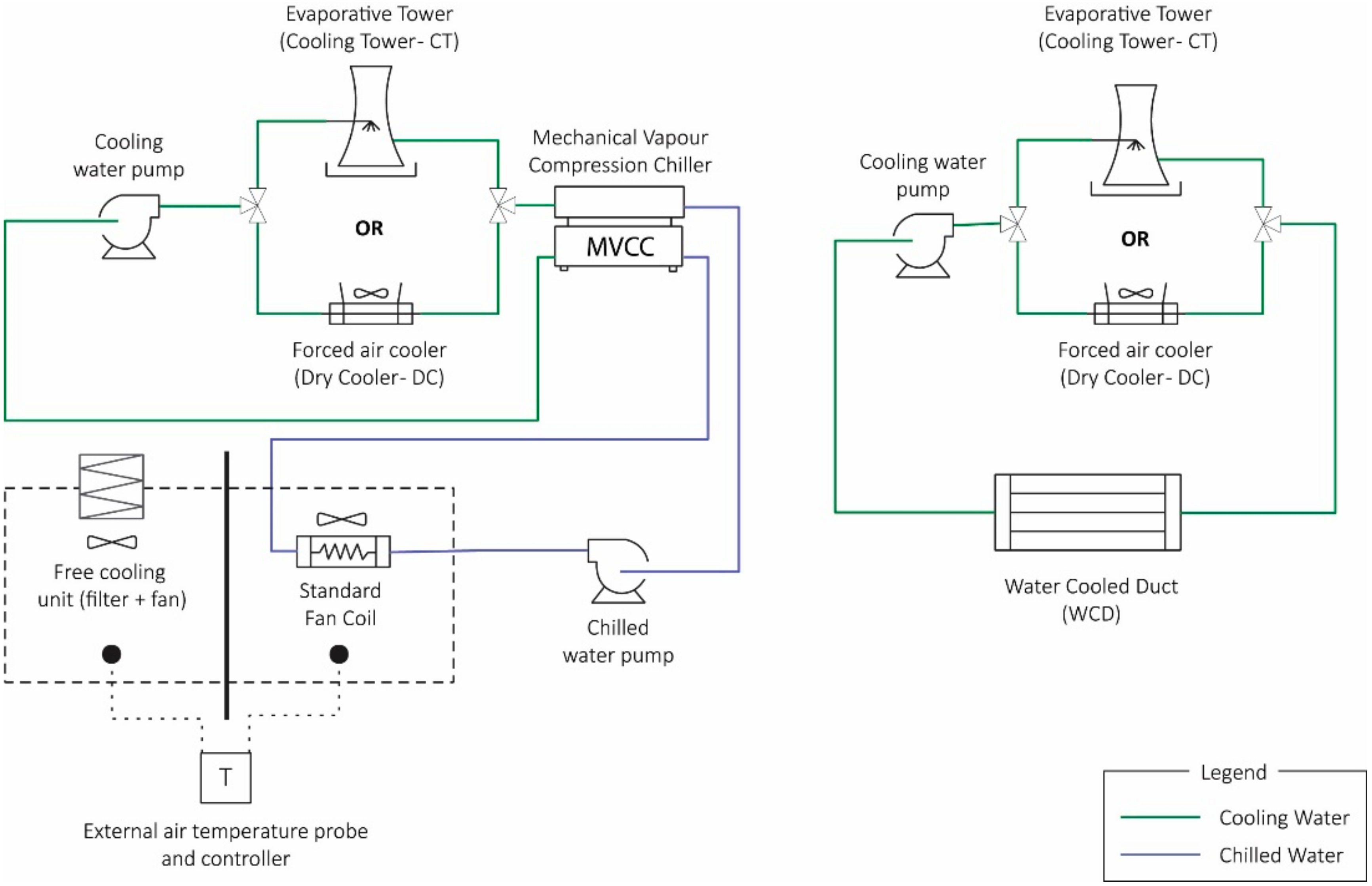
2.2. Cooling Systems Configurations

Three alternative cabin air conditioning configurations are modelled and compared in this study: the baseline mechanical vapour compression chiller (MVC) described in Section 2.2.1; an energy-saving mechanical vapour compression configuration based on airside free cooling with outside air (FC), presented in Section 2.2.2; and a waste heat recovery absorption-cooling-based configuration (ABS), as specified in Section 2.2.3. In particular, as in [5] and [9], it is proposed to recover waste heat from the hot gas line cooling system of conventional electric arc furnaces based on the plant layout and temperature profiles reported in [9]. In fact, in conventional EAFs, off-gases leaving the furnace and the following dropout box are cooled down to at least 600 °C, as required for the operation of subsequent plant components, by flowing through a modular gas-tight water-cooled duct [5,35], known in the industry as a WCD. In conventional configurations, the water used as refrigerant in the WCD needs to be cooled down in heat rejection units (i.e., either DC or CT). Total removed heat loads vary over time due to process intermittence, and depending on steelworks capacity, reaching values ranging between 10 and 20 MW for a 130 t nominal tap weight furnace [36]. For the heat recovery system of concern, we considered the opportunity to derive a water flow from a module of the cooling water circuit corresponding to an average heat flow of about 3100 kW. To obtain a simple and homogenous assessment of the impact of heat rejection units depending on climate, it was assumed that the same technology (i.e., either DC or CT) was used both for heat rejection at the WCD and as condenser for cabin refrigeration cycles.

2.2.1. Water-Cooled MVC Chiller

Mechanical vapour compression chillers are the most common refrigerators for air-conditioning purposes. In this study a water-cooled magnetic centrifugal chiller was selected as baseline refrigeration system for electric cabin air conditioning. The nominal capacity installed was 1300 kW and the performance was taken from a York catalogue for chillers [37]. The EER was 6.4, evaluated at an entering/leaving chilled water temperature of 12/7 °C and entering/leaving condenser water temperature of 30/35 °C.
Figure 1 shows the scheme of this configuration, which depicts both the cabin air conditioning system and the module of the WCD cooling circuit selected for heat recovery in configuration 2.2.3.

2.2.2. Free Cooling and MVC chiller

The FC configuration analysed in this paper, represented in Figure 2, consists of an MVC air conditioning configuration coupled with an external air ventilation system which draws air from outside and, after filtering, directly introduces it into the cabin, thereby reducing the cooling load for the conventional MVC chiller. In order to reduce the computational load without losing the significance in comparison, a fixed value of external air temperature was chosen to control the operation of the free cooling system. A value of 18 °C was assumed as the switch-off temperature, allowing the capacity of the free cooling ventilation system to be comparable with the internal fans’ capacity. Thus, when the external air temperature is higher than 18 °C, the standard MVC chiller operates to cool the internal cabin air. Otherwise, the system operates in FC mode. Also in this case, no heat recovery from the WCD occurs and its full load is dissipated at heat rejection units.

2.2.3. Air-Cooler and Water-Cooled ABS Chiller

The waste-heat-recovery-based cooling system represented in Figure 3 relies on a hot-water-fed single effect absorption chiller. As underlined in [5], in conventional WCDs at EAFs, due to no further utilization purposes of the emitted thermal energy, the cooling water outlet temperature is usually in the range of 50 °C [38]. If thermal energy recovery is considered, the design temperature of the cooling system has to be increased.
While it is also feasible to increase it to 200 °C, as demonstrated in [5], for this absorption cooling application the choice was made to increase it only to the average value of 90 °C. In this way, the system was designed to operate with hot water, in order to avoid introducing additional complexities from steam operation, such as additional maintenance and safety requirements related to higher temperature, pressure and phase change, which would be an additional burden in EAF plants without or with minimal steam networks. With hot water, single effect absorption chillers are used, whose reference EER is in the order of 0.7, in accordance with manufacturers’ catalogues [39,40] and the literature [21]. A commercial absorption cooling system with a nominal capacity of 1319 kW was assumed to be installed, based on the LG Absorption Chiller catalogue [40]. At EAF steelmaking sites where steam networks exist, an integrated development of heat-recovery-based steam generation as in [5] and of absorption-based cooling could be considered in order to exploit more efficient double effect absorption cycles [18,26]. However, this is beyond the scope of the present paper. Given the intermittence of the EAF melting process, based on the aforementioned tap-to-tap cycle, variations in flue gas temperatures correspond to oscillations in cooling water temperature at the heat recovery outlet. Thus, as in [5] and [9] a water storage tank is used as a hot water reservoir to compensate for power-off phases by limiting the temperature variability, which for single effect absorption cooling purposes is deemed acceptable in the range of 85 to 95 °C. The hot storage size was also designed to meet safety design criteria for cabin air conditioning systems, which imply that the cooling load to be removed from electric cabins was assumed to be constantly present during steelworks operations and to persist, during maintenance stops, for a period of three hours after the steelworks stop.

2.3. TRNSYS Simulation Model Development

TRNSYS [33] was used in this work to perform a dynamic simulation of the behaviour of the elements used in the various configurations analysed. TRNSYS libraries consist of components such as heating, ventilation and air conditioning (HVAC), electronics, controls, hydronics, etc. The elements are called types, and can be linked to others to simulate entire systems.
Dynamic system simulation is possible by including performance data and simulation parameters for individual elements. The configurations defined in Section 2 were modelled in TRNSYS based on the schematic diagrams shown in Figure 1, Figure 2 and Figure 3, obtaining TRNSYS input files (usually referred to as decks). As an example, the TRNSYS deck for the ABS configuration is represented in Figure 4.
The mass flowrates of chilled water and condenser water required by chillers were taken from manufacturers’ catalogues. MVC and ABS systems were simulated using technical data (reference chilled, cooling, and hot water flow rates) from the manufacturers’ catalogues [37] and [40], respectively, and the TRNSYS inbuilt performance data file, which allows EER simulation as a function of cooling, chilled, and hot water temperatures. The hot water tank was a stratified, five-layer adiabatic liquid storage tank simulated using TRNSYS type60. Cooling water from CTs or DCs served as input for the chiller condenser while the water leaving the chiller condenser was used as the input in CTs or DCs depending on the configuration studied. For the simulation of heat rejection units, technical data required as TRNSYS input were taken from LU-VE catalogue [41] and YWCT catalogue [42] for DCs and CTs, respectively.
A weather data file derived from the EnergyPlus weather database [43] was provided as input to CT, DC, and the cabin building to capture the effect of external environment conditions. Climate zones were selected according to ASHRAE [34]. Table 1 shows the cities selected here to represent each climate zone and their climate characteristics. The three cooling configurations described in the previous section were simulated in 16 out of 17 of the selected cities. Climate zone number 8 was not considered for simulations since cooling towers are inoperable in this zone [32] due to the extremely low temperatures (see Table 1). Therefore, a total of 96 simulations were performed.

2.4. Calculation of Water–Energy–Greenhouse Gas (GHG) Nexus Indicators

In accordance with [9,44], the total blue water footprint, carbon footprint and primary energy demand were selected as water–energy–carbon nexus indicators in this analysis. They meet most requirements reported by [45,46] for sustainability indicators; in particular, they are easy to interpret, able to show trends over time and sensitive to changes in the systems analysed here (i.e., different configurations of cabin refrigeration systems).

2.4.1. Water Footprint

The total water footprint Wf was calculated as the sum of the water consumption within systems (direct water use, Wd) and the water footprint of energy consumed (indirect water use, Wind) according to Equation (1):
W f = W d + W i n d = k · W e v + C W , e l E e l .
In the present evaluation, we did not account for water pollution impacts (so-called grey water), but only for blue water footprint, which measures the consumptive use of surface and ground water.
Direct water consumption only occurs in CT configurations due to evaporation loss, drift and makeup-water requirements. Evaporated quantities were calculated with TRNSYS [33] using type51b. Additional water losses due to bleed off and drift were quantified as in [9] using a multiplicative coefficient k on the evaporated water Wev, taking k = 2 as a reasonable estimate [47]. The footprint calculation approach and the data sources reported in [9] were used to derive the indirect water consumption rate CW,el for each reference city based on the national electricity production mix reported in Table 2, elaborated from the WorldBank database [48].
The total electricity demand Eel was determined as the sum of the energy required for each component simulated in TRNSYS. The chiller performance was considered in the energy consumption calculation by using the corresponding TRNSYS types. In-built TRNSYS performance data files were used to evaluate the EER and consequently the energy consumption, which is related to the cooling water temperature returning from the heat rejection device (DC or CT) as well as the temperature of chilled outlet water. For the absorption chiller, the inlet hot water temperature was also introduced as parameter to determine the EER. As a result, the yearly average EER values obtained from simulations in the climate regions of concern ranged between 0.52 and 0.55 for absorption cooling systems, and between 5.24 and 9.61 for compression cooling systems.

2.4.2. Carbon Footprint and Primary Energy Demand Calculation

Carbon footprint has been defined as “the quantity of GHGs expressed in terms of CO2 equivalent mass emitted into the atmosphere by an individual, organization, process, product or event from within a specified boundary” [49].
As in the case of water footprint, differences in the carbon footprint of the configurations examined are exclusively bound to electricity consumption, since none of the air conditioning alternatives examined implies any direct fuel consumption. Carbon footprint was thus calculated according to Equation (2).
C O 2 f = C O 2 i n d = C C O 2 , e l E e l .
On the other hand, based on the data sources used in this study (see [9]), carbon footprint coefficients for electricity consumption CCO2,el were estimated with a life cycle approach (i.e., all CO2eq emissions consumption from extraction to plant construction were considered).
In a similar manner to [50], in this study it was assumed that the changes in direct carbon equivalent emissions from refrigerant leaks induced by switching from vapour compression units to absorption cooling systems were negligible compared to the emissions of greenhouse gases embodied in purchased electricity.
The primary energy consumption associated with purchased electricity was calculated according to Equation (3):
P E D = C P E D , e l E e l .
Site-to-source energy conversion factors C P E D , e l reported in Table 2 were obtained with the methodology and data sources discussed in [9,51] based on national energy mix data reported in Table 2.

2.5. Basis for Economic Assessment

The life cycle cost was used as a basis for economic assessment. According to the scheme proposed in [46], life cycle costs of buildings under an energy efficiency assessment framework may include initial, operation, repair, spare, downtime, loss, maintenance (corrective, preventive and predictive) and disposal costs. Based on available data, only initial (capital) costs of installations and operational costs of electricity and of water were considered.
For each configuration, the life cycle cost (LCC) for an interest rate of 10% and a lifetime of 10 years was calculated using the standard formula:
L C C = C o p q n 1 q n · i + C c a p ,
where:
-
C o p is the operating cost.
-
C c a p is the plant capital cost.
-
i is the interest rate.
-
n is the useful life of the plant.
-
q   =   1   +   i .
A payback analysis was also later introduced to compare the economic feasibility between ABS and FC configurations. The payback period (PB) was evaluated using the following formula:
P B = C p , A B S C p , F C C o , F C C o , A B S ,
where:
-
C p , A B S is the plant cost of the ABS configuration.
-
C p , F C is the plant cost of the FC configuration.
-
C o , F C is the operating (energy and water) cost of FC alternatives.
-
C o , A B S is the operating (energy and water) cost of ABS alternatives.
One should bear in mind that the simple payback time calculated according to Equation (5) allows a direct comparison between ABS and FC alternatives, but does not account for interest rates, which may lead to slightly different results with respect to LCC-based comparisons.
Capital cost estimates for absorption cooling systems, mechanical vapour compression cooling systems, dry coolers and cooling towers were obtained from the cost functions reported in [9], summarized in Table 3.
The operational expenses for different configurations were mainly determined by electricity consumption and—for CT configurations—by water consumption. It was not possible to retrieve electricity and industrial water prices all over the world. To obtain an approximate estimate for reasonable ranges, Western European values were derived from [9] as guide values, and are reported in Table 4.

3. Results and Discussion

3.1. Average Total Cabin Cooling Load

Figure 5 shows the total cooling load, averaged over operating hours of one year, for the reference electric cabin in the climate zones of interest. On a yearly basis, heat transfer through the cabin envelope led to lower cooling loads, particularly in colder climates. However, the difference between the average cooling load in climate 7 (cold) and in climate 1A (hot) Was less than 3% of the total cooling load.

3.2. Electric Energy Consumption

For each configuration, Figure 6 shows the annual electric energy consumption of the whole system (i.e., including cabin cooling as well as waste heat management from the WCD within the system boundaries). In Figure 6, Figure 7, Figure 8 and Figure 9, the results are represented as histograms for each climate zone, in two rows (sub-figures) depending on the condenser used (with DC above and CT below). The bars labelled as BASE, FC, and ABS corresponding to the traditional MVC, free cooling, and absorption cooling configurations, respectively.
In Figure 6, the electricity demand by auxiliaries (AUX) is represented in green scale at the base of the bars, the demand for cabin refrigeration (REF) is represented by the intermediate bars in blue scale, while the top bars in yellow scale correspond to the electricity demand for heat dissipation from the WCD of the EAF. The relative reduction of electricity consumption in the ABS cooling mode compared with the baseline was on the order of 40% to 60%, and was more evident in CT configurations, which inherently require less electric power than DC to dissipate the same heat flows. In the FC configuration, which does not include waste heat recovery, the electricity consumption for heat dissipation at the WCD remained unchanged from baseline.
The reduction in electricity consumption for refrigeration was more pronounced in FC than in ABS configuration in several climatic regions, but almost exclusively when DCs were used. In fact, the overall balance resulted in a slight to remarkable advantage for ABS in all but the last climates in CT configurations, whereas in DC configurations FC outperformed the ABS configuration in climate zones 4C (mixed-marine), 5A (cool-humid), 5C (cool-marine) and 7. Interestingly enough, in continental dry climates such as in Dunhuang (5B) and Helena (6B), prolonged high-temperature periods in summer reduced the contribution of FC to electric energy saving over the year, making ABS cooling more attractive in terms of electricity demand.

3.3. Direct and Indirect Water Consumption

Water consumption is illustrated in Figure 7. DC configurations imply only indirect water consumption, which was small and basically mirrored electricity consumption patterns, in a more or less pronounced way depending on the water intensity of the local electricity generation mix (see Table 2). In other words, this means that when DCs were used as heat dissipation systems, ABS configurations were mostly preferable to FC configurations also as to their impact on freshwater consumption.
For CT configurations, the direct water consumption (at the base of bars, in blue) was several orders of magnitude larger than the indirect consumption. Nevertheless, their overall balance was significantly affected by the indirect water footprint: for instance, although the direct water consumption of CTs evidently decreased in colder climates, the total water footprint of the baseline CT configuration in Östersund (climate region 7) equalled the baseline in Cairo (climate region 2B) due to the high indirect water footprint of electricity in Sweden.
For CT configurations, FCs were usually best performers in terms of direct freshwater footprint. In fact, the direct water consumption of FC configurations was always lower than that of corresponding ABS systems, except in very hot humid climates (1A). Indeed, the ABS configuration generally had a direct water consumption lower than or equal to the baseline, and its total (i.e., direct plus indirect) freshwater footprint was always lower than the baseline. However, FC configurations, in spite of their higher electricity demand, generally outperformed ABS cooling in terms of overall freshwater footprint, which was lower for the ABS configuration only in Singapore (1A) and New Delhi (1B). For New Delhi, this was mainly due to the high indirect water consumption associated with the national electricity mix, which is rich in water-intensive solid-fuel-based power generation (Table 2).

3.4. Direct and Indirect CO2 Emissions

CO2 footprints are compared in Figure 8. Only indirect CO2 emissions associated with electricity consumption characterized the systems of interest. Hence, the CO2 emission performance of configurations reflects electricity consumption both for DC and CT configurations. Indeed, the influence of the national energy mix on carbon emission was remarkable: for instance, baseline DC configurations achieved similar performance in Birmingham and Cairo, although their electricity consumption would be about 15% higher in the latter city (see Figure 6). Nevertheless, the climate dependence trend demonstrated for electricity (Figure 6) was basically conserved for CO2 emissions (Figure 8): heat-recovery-based ABS cooling outperformed FC in all but the last CT configuration and in very hot to mixed climate zones, as well as in cool climates with hot summers, for DC configurations.

3.5. Primary Energy Consumption

The primary energy consumption trends represented in Figure 9 basically followed the CO2 footprint trends. Comparing Figure 8 and Figure 9, slight differences in the trends were observed in regions with higher shares of nuclear energy (e.g., Taipei—2A, Lyon—4A, Seoul—4B, Östersund—7), which has minimal GHG emissions but a high primary energy factor according to reference [45].

3.6. Economic Performance

The LCCs of alternative cooling systems configurations are compared in Figure 10.
It is interesting to observe that at the resource cost conditions considered (average conditions, labelled as “Mean” in Table 4), the life cycle costs for configurations using CTs were slightly higher than corresponding configurations using DCs. In the long run, the lower capital costs and lower electricity cost of CT-based solutions did not compensate the additional economic impact of water consumption.
The proposed FC strategy requires few components and a simple regulation, which means that, compared with the baseline, additional investments are basically negligible. As a consequence, the life cycle costs of FC configurations were always lower than those of corresponding MVC configurations.
The proposed waste-heat to cooling ABS configuration requires significant investment but generates major savings in electricity costs and—for CT configurations—small savings in water costs in most climates. As a result, the life cycle costs of ABS configurations at average price conditions were always lower than those of corresponding MVC configurations, but in some climate regions (4C, 5A, 5C, 6A, 6B, 7 with either DCs or CTs, and also in 4A with CTs) they were higher than those of FC configurations, as shown in Figure 10.
This is highlighted more generally in Figure 11, which shows the simple payback time (PBT) of ABS with respect to corresponding FC configurations according to Equation (5). Figure 11 also shows the dependence of PBT on climate zones, electricity prices and, for CT configurations, on water prices. In particular, Figure 11a shows the sensitivity of the economic performance of ABS with DC to the electricity price by presenting PBTs at minimum, mean and maximum levels of electricity price according to Table 4. Similarly, Figure 11b shows the sensitivity of PBTs in the ABS with CT configuration to the electricity price and Figure 11c shows the sensitivity of PBTs in the ABS with CT configuration to the water price (at the minimum, mean and maximum levels reported in Table 4). It can be observed that lower electricity prices resulted in smaller savings and consequently longer payback periods, which stretched even beyond the investment time horizon for CT configurations from climate zone 3C and subsequent. Similarly, high water prices in CT configurations increased operational expenses of ABS configurations, and hence led to longer payback times. Grey areas, corresponding to regions 4C, 5A, 5C, 6A and 7 with either DCs or CTs, and also in 6B with CTs) indicate the climate zones where the electricity consumption of ABS configuration was mostly higher than that of FC configuration: depending on price levels, the payback times of ABS configurations in these cases would either be negative (i.e., ABS never pays off) or at least longer than the system’s service life.
It can be observed that:
-
ABS cooling was more cost effective than FC in most climates and paid off in less than three years even at worst (i.e., lowest) electricity price conditions in very hot to warm dry or humid climate zones, both in DC and CT configurations;
-
Where DCs are used (e.g., due to general water scarcity), ABS cooling may be a more rewarding option than FC even in mixed to cool dry climate zones (4B and 5B). Similar paybacks were also achieved with DC in warm marine climate zones (3C), however it should be noted that if industries are placed directly by the sea-coast, other resource-efficient heat rejection options may be used (e.g., once-through cooling) which are beyond the scope of the present research;
-
ABS CT configurations, featuring lower electricity consumption and absolute electric energy savings than DC, had slightly longer PBTs, which were nevertheless satisfactory (i.e., lower than three years) in very hot to warm dry climates, and in unfavourable economic conditions (low electricity prices or high water prices).
-
The economic performance of ABS systems with CTs was more sensitive to electricity price in hot climates, and to water prices in mixed to cool dry climates where FC enables substantial water savings compared with ABS cooling (see Figure 7).

4. Conclusions

In this study, the energy, water, CO2 and primary energy consumption of different configurations of air conditioning systems for electric cabins were analysed considering 16 ASHRAE climate zones worldwide. The case at hand refers to electric cabins of EAF steelmaking sites, but the methodology and general results could be easily extended to similar installations in process industries having considerable low-grade waste heat flows.
It was confirmed that the proposed waste heat utilization system for absorption cooling allowed substantial energy savings and an overall favourable water–energy–GHG balance in all climate zones compared with traditional mechanical vapour compression air cooling systems for electric cabins. Compared with the simple airside free cooling configuration proposed here, absorption cooling was also the better option as to electric energy consumption in nearly all climate zones (15 out of 16 climate zones for systems with cooling towers and 12 out of 16 climate zones for systems with dry coolers as heat rejection units). A similar trend was observed for GHG emissions and primary energy demand, which had more or less pronounced differences depending on the local electricity generation mix of the analysed locations. In some cases, such indicators were shown to be more heavily affected by the country’s energy mix than by climatic conditions.
However, it was shown that in configurations using cooling towers, free cooling led to significantly lower direct water consumption in nearly all climate regions, and to a lower overall water footprint, particularly in mixed to very cold climates. In climate regions 4B to 7, free cooling was also more cost effective than waste-heat recovery for the examined ranges of economic parameters. In those regions, free cooling also allowed substantial energy savings, though lower than those of corresponding absorption cooling solutions.
Hence, in general terms, our results indicate that waste heat recovery for electric cabin cooling is an energy efficient solution which is also water efficient when dry cooling systems are used. In systems with cooling towers, it generally decreases the system’s water footprint compared with baseline configurations, but not with free cooling alternatives. Under the technical and market conditions examined in this paper, absorption cooling was clearly the least cost option for electric cabin cooling in warm to very hot climate zones, but where CTs are used it is the most water-efficient option only in very hot dry climates.
Due to the better performance of absorption cooling in terms of energy and carbon footprint, even in cold climates and with a low-carbon national energy generation mix, carbon- or energy-efficient incentives could make it economically feasible also in further climate regions (e.g., in mixed climate zones), even for systems using cooling towers and at high water prices. In that case, industrial designers and energy managers might prefer absorption cooling solutions because of their energy efficiency even where, compared with FC, they are suboptimal in terms of water consumption.
It is thus recommended that, particularly in intermediate climate conditions, decision makers accurately evaluate the water footprint of their energy efficiency projects; the approach proposed in the current analysis could support them in this task. It is also desirable that policy makers who design incentives supporting industrial energy efficiency or GHG reduction combine them with constraints or incentives for water consumption reduction, taking a nexus approach.

Author Contributions

Conceptualization: D.C. and O.S.; Methodology: collectively developed by all authors; Investigation: M.S. and A.Z.; Software and Visualization: M.S. and A.Z.; Supervision: D.C., O.S. and A.D.A.; Writing—original draft: D.C. and M.S.; Writing—review and editing: O.S., A.Z. and A.D.A.

Funding

This research received no external funding.

Conflicts of Interest

The authors declare no conflict of interest.

Nomenclature

ABS(C)Absorption Chiller
AUXElectricity demand by auxiliaries
BFBlast Furnace
BOFBasic Oxygen Furnace
C O 2 f Total CO2 footprint—tons
C O 2 i n d Total CO2 indirect emissions—tons
C C O 2 , e l Carbon footprint coefficients for electricity consumption (tCO2/GWh)
C i n v Plant investment cost (EURO)
C o p Operating cost (EURO/year)
C o , A B S ABS configuration operating cost (EURO/year)
C o , F C FC configuration operating cost (EURO/year)
C P E D , e l Site-to-source energy conversion factors (TOE/GWh)
C p , A B S Plant cost of ABS configuration (EURO)
C p , F C Plant cost of FC configuration (EURO)
C W , e l Indirect water consumption rate (m3/GWh)
CTCooling Tower
COPCoefficient of Performance
DCDry Coolers
EAFElectric Arc Furnace
E e l Total electricity demand (GWh)
EEREnergy Efficiency Ratio
ETSEmission Trading Schemes
EUEuropean Union
FCFree Cooling
GHGGreenhouse Gas
HVACHeating, Ventilation and Air Conditioning
i Interest rate (%)
IWHIndustrial Waste Heat
k Multiplicative coefficient for water losses due to bleed off and drift—dimensionless
MVC(C)Mechanical Vapour Compression Chiller
n Life of the plant (years)
ORCOrganic Rankine Cycle
PEDPrimary Energy Demand (consumption) (TOE)
PB Payback Period (years)
PBTPayback Time
q Defined as 1 + i
REFRefrigeration
TOETon (of) Oil Equivalent
WCDWater Cooled Duct
WENWater Energy Nexus
W d Direct water use (m3)
W e v Evaporated water (m3)
W f Total water footprint (m3)
W i n d Indirect water use (m3)

References

  1. He, K.; Wang, L. A review of energy use and energy-efficient technologies for the iron and steel industry. Renew. Sustain. Energy Rev. 2017, 70, 1022–1039. [Google Scholar] [CrossRef]
  2. IEA. World Energy Outlook 2010; International Energy Agency: Paris, France, 2010; Available online: https://webstore.iea.org/world-energy-outlook-2010 (accessed on 17 June 2019).
  3. European Union. European Commission, EU-ETS Handbook 2015. Available online: https://ec.europa.eu/clima/sites/clima/files/docs/ets_handbook_en.pdf (accessed on 17 June 2019).
  4. Huisingh, D.; Zhang, Z.; Moore, J.C.; Qiao, Q.; Li, Q. Recent advances in carbon emissions reduction: Policies, technologies, monitoring, assessment and modeling. J. Clean. Prod. 2015, 103, 1–12. [Google Scholar] [CrossRef]
  5. Keplinger, T.; Haider, M.; Steinparzer, T.; Patrejko, A.; Trunner, P.; Haselgrübler, M. Dynamic simulation of an electric arc furnace waste heat recovery system for steam production. Appl. Therm. Eng. 2018, 135, 188–196. [Google Scholar] [CrossRef]
  6. Schnoor, J. Water-energy nexus. Environ. Sci. Technol. 2011, 45, 5065. [Google Scholar] [CrossRef] [PubMed]
  7. World Steel Association. Water Management in the Steel Industry 2015; Position Paper; WSA AISBL: Brussels, Belgium, 2015; ISBN 978-2-930069-81-4. Available online: https://www.worldsteel.org/en/dam/jcr:f7594c5f-9250-4eb3-aa10-48cba3e3b213/Water+Management+Position+Paper+2015.pdf (accessed on 17 June 2019).
  8. Wang, C.; Zheng, X.; Cai, W.; Gao, X.; Berrill, P. Unexpected water impacts of energy-saving measures in the iron and steel sector: Tradeoffs or synergies? Appl. Energy 2017, 205, 1119–1127. [Google Scholar] [CrossRef]
  9. Chinese, D.; Santin, M.; Saro, O. Water-energy and GHG nexus assessment of alternative heat recovery options in industry: A case study on electric steelmaking in Europe. Energy 2017, 141, 2670–2687. [Google Scholar] [CrossRef] [Green Version]
  10. Gao, C.; Wang, D.; Dong, H.; Cai, J.; Zhu, W.; Du, T. Optimization and evaluation of steel industry’s water-use system. J. Clean. Prod. 2011, 19, 64–69. [Google Scholar] [CrossRef]
  11. Gu, Y.; Xu, J.; Keller, A.A.; Yuan, D.; Li, Y.; Zhang, B.; Wenig, Q.; Zhang, X.; Deng, P.; Wang, H.; et al. Calculation of water footprint of the iron and steel industry: A case study in Eastern China. J. Clean. Prod. 2015, 92, 274–281. [Google Scholar] [CrossRef]
  12. Moya, J.A.; Pardo, N. The potential for improvements in energy efficiency and CO2 emissions in the EU27 iron and steel industry under different payback periods. J. Clean. Prod. 2013, 52, 71–83. [Google Scholar] [CrossRef]
  13. Johansson, M.T.; Söderström, M. Options for the Swedish steel industry energy efficiency measures and fuel conversion. Energy 2011, 36, 191–198. [Google Scholar] [CrossRef]
  14. Lin, Y.P.; Wang, W.H.; Pan, S.Y.; Ho, C.C.; Hou, C.J.; Chiang, P.C. Environmental impacts and benefits of Organic Rankine Cycle power generation technology and wood pellet fuel exemplified by electric arc furnace steel industry. Appl. Energy 2016, 183, 369–379. [Google Scholar] [CrossRef]
  15. Lee, B.; Sohn, I. Review of innovative energy savings technology for the electric arc furnace. JOM 2014, 66, 1581–1594. [Google Scholar] [CrossRef]
  16. Xu, Z.; Wang, R. Absorption refrigeration cycles: Categorized based on the cycle construction. Int. J. Refrig. 2016, 62, 114–136. [Google Scholar] [CrossRef]
  17. Sun, J.; Fu, L.; Zhang, S. A review of working fluids of absorption cycles. Renew. Sustain. Energy Rev. 2012, 16, 1899–1906. [Google Scholar] [CrossRef]
  18. Banu, P.A.; Sudharsan, N. Review of water based vapour absorption cooling systems using thermodynamic analysis. Renew. Sustain. Energy Rev. 2018, 82, 3750–3761. [Google Scholar] [CrossRef]
  19. Shirazi, A.; Taylor, R.A.; Morrison, G.L.; White, S.D. Solar-powered absorption chillers: A comprehensive and critical review. Energy Convers. Manag. 2018, 171, 59–81. [Google Scholar] [CrossRef]
  20. Wang, J.; Yan, R.; Wang, Z.; Zhang, X.; Shi, G. Thermal Performance Analysis of an Absorption Cooling System Based on Parabolic Trough Solar Collectors. Energies 2018, 11, 2679. [Google Scholar] [CrossRef]
  21. Eicker, U. Energy Efficient Buildings with Solar and Geothermal Resources; John Wiley & Sons: Hoboken, NJ, USA, 2014. [Google Scholar]
  22. Viklund, S.B.; Johansson, M.T. Technologies for utilization of industrial excess heat: Potentials for energy recovery and CO2 emission reduction. Energy Convers Manag. 2014, 77, 369–379. [Google Scholar] [CrossRef]
  23. Xia, L.; Liu, R.; Zeng, Y.; Zhou, P.; Liu, J.; Cao, X.; Xiang, S. A review of low-temperature heat recovery technologies for industry processes. Chin. J. Chem. Eng 2018. In Press, Corrected Proof. [Google Scholar] [CrossRef]
  24. Liew, P.Y.; Walmsley, T.G.; Alwi, S.R.W.; Manan, Z.A.; Klemeš, J.J.; Varbanov, P.S. Integrating district cooling systems in locally integrated energy sectors through total site heat integration. Appl. Energy 2016, 184, 1350–1363. [Google Scholar] [CrossRef]
  25. Leong, Y.T.; Chan, W.M.; Ho, Y.K.; Isma, A.I.M.I.A.; Chew, I.M.L. Discovering the potential of absorption refrigeration system through industrial symbiotic waste heat recovery network. Chem. Eng. Trans. 2017, 61, 1633–1638. [Google Scholar]
  26. Brückner, S.; Liu, S.; Miró, L.; Radspieler, M.; Cabeza, L.F.; Lävemann, E. Industrial waste heat recovery technologies: An economic analysis of heat transformation technologies. Appl. Energy 2015, 151, 157–167. [Google Scholar] [CrossRef]
  27. Cola, F.; Romagnoli, A.; Hey, J. An evaluation of the technologies for heat recovery to meet onsite cooling demands. Energy Convers. Manag. 2016, 121, 174–185. [Google Scholar] [CrossRef]
  28. Haywood, A.; Sherbeck, J.; Phelan, P.; Varsamopoulos, G.; Gupta, S.K. Thermodynamic feasibility of harvesting data centre waste heat to drive an absorption chiller. Energy Convers. Manag. 2012, 58, 26–34. [Google Scholar] [CrossRef]
  29. Ebrahimi, K.; Jones, G.F.; Fleischer, A.S. A review of data centre cooling technology, operating conditions and the corresponding low-grade waste heat recovery opportunities. Renew. Sustain Energy Rev. 2014, 31, 622–638. [Google Scholar] [CrossRef]
  30. Oró, E.; Depoorter, V.; Pflugradt, N.; Salom, J. Overview of direct air free cooling and thermal energy storage potential energy savings in data centres. Appl. Therm. Eng. 2015, 85, 100–110. [Google Scholar] [CrossRef]
  31. Daraghmeh, H.M.; Wang, C.C. A review of current status of free cooling in datacentres. Appl. Therm. Eng. 2017, 114, 1224–1239. [Google Scholar] [CrossRef]
  32. Agrawal, A.; Khichar, M.; Jain, S. Transient simulation of wet cooling strategies for a data centre in worldwide climate zones. Energy Build. 2016, 127, 352–359. [Google Scholar] [CrossRef]
  33. Thermal Energy System Specialists LLC—TRNSYS 17 Documentation, Mathematical Reference. Available online: http://web.mit.edu/parmstr/Public/TRNSYS/04-MathematicalReference.pdf (accessed on 17 June 2019).
  34. ASHRAE. ASHRAE/IESNA 90.1 Standard-2007-Energy Standard for Buildings Except Low-Rise Residential Buildings; American Society of Heating Refrigerating and Air-conditioning Engineers: New York, NY, USA, 2007. [Google Scholar]
  35. Pansera, G.; Griffini, N. Dedusting plants for electric arc furnaces. Millenn. Steel. 2016, 85–89. Available online: http://millennium-steel.com/wp-content/uploads/articles/pdf/2005/pp85-89%20MS05.pdf (accessed on 17 June 2019).
  36. Kühn, R.; Geck, H.G.; Schwerdtfeger, K. Continuous off-gas measurement and energy balance in electric arc steelmaking. ISIJ Int. 2005, 45, 1587–1596. [Google Scholar] [CrossRef]
  37. Johnson Controls. York® Commercial & Industrial HVAC 2016; Johnson Controls: Milwaukee, WI, USA, 2017; Available online: http://www.clima-trade.com/Download/be_york_chillers_and_heatpumps_en_2016.pdf (accessed on 17 June 2019).
  38. Mombeni, A.G.; Hajidavalloo, E.; Behbahani-Nejad, M. Transient simulation of conjugate heat transfer in the roof cooling panel of an electric arc furnace. Appl. Therm. Eng. 2016, 98, 80–87. [Google Scholar] [CrossRef]
  39. Johnson Controls. York® YIA Absorption Chiller Engineering Guide; Johnson Controls: Milwaukee, WI, USA, 2017; Available online: https://www.johnsoncontrols.com/-/media/jci/be/united-states/hvac-equipment/chillers/be_engguide_yia_singleeffect-absorption-chillers-steam-and-hot-water-chillers.pdf (accessed on 17 June 2019).
  40. LG Electronics. LG HVAC Solution Absorption Chiller. 2018. Available online: https://www.lg.com/global/business/download/resources/CT00022379/CT00022379_28284.pdf (accessed on 17 June 2019).
  41. LU-VE/AIA. Dry Coolers and Condensers for Industrial Applications. 2017. Available online: https://manuals.luve.it/Industrial%20Applications/files/assets/common/downloads/Industrial%20Applications.pdf (accessed on 17 June 2019).
  42. YWCT. YWCT Cooling Tower Catalogue. 2010. Available online: http://www.customcoolingtowers.com/_Uploads/dbsAttachedFiles/YWCT_Catalog_2010_2.pdf (accessed on 17 June 2019).
  43. Energy Plus Climate Database. 2018. Available online: https://energyplus.net/ (accessed on 17 June 2019).
  44. Chhipi-Shrestha, G.; Kaur, M.; Hewage, K.; Sadiq, R. Optimizing residential density based on water–energy–carbon nexus using UTilités Additives (UTA) method. Clean Technol. Environ. Policy 2018, 20, 855. [Google Scholar] [CrossRef]
  45. Waas, T.; Hugé, J.; Block, T.; Wright, T.; Benitez-Capistros, F.; Verbruggen, A. Sustainability assessment and indicators: Tools in a decision-making strategy for sustainable development. Sustainability 2014, 6, 5512–5534. [Google Scholar] [CrossRef]
  46. Danish, M.S.S.; Senjyu, T.; Ibrahimi, A.M.; Ahmadi, M.; Howlader, A.M. A managed framework for energy-efficient building. J. Build. Eng. 2019, 21, 120–128. [Google Scholar] [CrossRef]
  47. REA, Inc. Cooling Tower Make-up Water Flow Calculation. Available online: http://www.reahvac.com/tools/cooling-tower-make-water-flow-calculation/ (accessed on 17 September 2019).
  48. World Bank Database. World Development Indicators: Electricity Production, Sources, and Access. Available online: http://www.tsp-data-portal.org/Breakdown-of-Electricity-Generation-by-Energy-Source#tspQvChart (accessed on 18 June 2019).
  49. Pandey, D.; Agrawal, M.; Pandey, J.S. Carbon footprint: Current methods of estimation. Environ. Monit. Assess. 2011, 178, 135–160. [Google Scholar] [CrossRef] [PubMed]
  50. Meunier, F. Co- and tri-generation contribution to climate change control. Appl. Therm. Eng. 2002, 22, 703–718. [Google Scholar] [CrossRef]
  51. Wilby, M.R.; Gonzalez, A.B.R.; Díaz, J.J.V. Empirical and dynamic primary energy factors. Energy 2014, 73, 771–779. [Google Scholar] [CrossRef]
Figure 1. Mechanical vapour compression chiller schematic diagram.
Energies 12 03627 g001
Figure 2. Mechanical vapour compression chiller with free cooling system schematic diagram.
Energies 12 03627 g002
Figure 3. Absorption chiller schematic diagram.
Energies 12 03627 g003
Figure 4. Absorption cooling (ABS) configuration modelled in TRNSYS. Dashed lines are used as control indicators.
Energies 12 03627 g004
Figure 5. Simulated average cabin load over 16 climate zones.
Energies 12 03627 g005
Figure 6. Electricity consumption based on climate zone and case study. AUX: electricity demand by auxiliaries; REF: demand for cabin refrigeration.
Energies 12 03627 g006
Figure 7. Direct and indirect water consumption based on climate zone and case study.
Energies 12 03627 g007
Figure 8. Indirect CO2 emission based on climate zone and case study.
Energies 12 03627 g008
Figure 9. Primary energy (PE) consumption based on climate zone and case study.
Energies 12 03627 g009
Figure 10. Life cycle cost (LCC) analysis based on climate zone and case study at mean electricity and water prices. CAP. is for plant capital costs, Elec. and Water are the life cycle operational expenses for electricity and water, respectively.
Energies 12 03627 g010
Figure 11. Payback times of ABS cooling solutions with respect to FC solutions depending on electricity and water prices (a) FC with DC, sensitivity to electricity price; (b) FC with CT, sensitivity to electricity price; (c) FC with CT, sensitivity to water price.
Energies 12 03627 g011aEnergies 12 03627 g011b
Table 1. Climate zones defined by ASHRAE and relative representative city. Zone number 8 (in italics) was not considered in this work.
Climate ZoneCityDRY BULB t. (°C)WET BULB t. (°C)RH (%)
MinMaxMeanMinMaxMeanMinMaxMean
1ASingapore21.133.827.516.928.225.14410084
1BNew Delhi5.244.324.7429.51999962
2ATaipei63822.85.12920.33510081
2BCairo742.921.762715.91010059
3AAlgiers−0.838.517.7-127.114.61310075
3BTunis1.339.918.81.226.815.21410072
3CAdelaide239.216.21.225.211.7610063
4ALyon−8.533.611.9−9.226.29.41610076
4BSeoul−11.832.711.9−13.329.69.2910069
4CAstoria−3.328.310.3−4.721.48.62910081
5AHamburg−8.5329−9.222.87.12610080
5BDunhuang−19.639.19.8−2024.33.649842
5CBirmingham−7.430.49.7−7.820.37.71910078
6AMoscow−25.230.65.5−25.221.73.72810077
6BHelena−29.436.16.8−29.719.12.51110057
7Ostersund−25.726.53.2−26.118.51.32310075
8Yakutsk−48.332.1−9.1−48.320−11.11410068
Table 2. National energy mix for the analysed countries (climates) in this paper [44]. TOE: ton (of) oil equivalent.
CityNationBiomass and WasteSolid FuelsNatural GasGeothermal EnergyHydropowerNuclear EnergyCrude OilSolar EnergyWind Energy C C O 2 , e l
(tCO2/GWh)
C W , e l
(m3H2O/GWh)
C P E D , e l
(TOE/GWh)
SingaporeSingapore1.39%0.00%79.77%0.00%0.00%0.00%18.82%0.02%0.00%5241105212
New DelhiIndia0.51%68.21%10.35%0.96%12.69%3.02%1.17%0.21%2.88%7456284228
TaipeiTaiwan1.45%32.65%10.88%0.00%2.40%16.55%35.32%0.01%0.73%6462510254
CairoEgypt0.00%0.00%74.59%0.00%8.70%0.00%15.73%0.15%0.83%4784189196
AlgiersAlgeria0.00%0.00%93.39%0.00%1.13%0.00%5.48%0.00%0.00%4901463202
TunisTunisia0.00%0.00%98.19%0.00%0.62%0.00%0.00%0.00%1.18%4731254197
AdelaideAustralia0.98%69.33%19.28%0.00%5.82%0.00%1.41%0.63%2.56%7993754235
LyonFrance0.98%3.99%3.60%0.00%10.89%76.33%0.57%0.84%2.79%825909245
SeoulSouth Korea0.24%42.36%23.03%0.00%0,79%29.03%4.14%0.22%0.18%5732094254
AstoriaUSA1.77%38.23%29.77%0.09%6.84%19.04%0.68%0.11%3.48%5384057227
HamburgGermany7.68%46.37%11.33%0.00%3.61%16.20%1.53%4.54%8.73%5412973221
DunhuangChina0.95%74.94%1.69%0.00%18.14%1.96%0.16%0.13%2.03%7648226223
BirminghamUK4.23%40.09%27.84%0.14%1.55%18.99%0.99%0.35%5.81%5502180232
MoscowRussia0.30%15.39%48.84%0.00%16.35%16.54%2.57%0.00%0.00%4157243202
HelenaUSA1.77%38.23%29.77%0.09%6.84%19.04%0.68%0.11%3.48%5384057227
ÖstersundSweden7.15%1.01%1.03%0.00%48.00%37.76%0.65%0.01%4.40%4018657155
YakutskRussia0.30%15.39%48.84%0.00%16.35%16.54%2.57%0.00%0.00%4157243202
Table 3. Equipment cost functions used in this work.
TechnologyCost Function Structure
(Y in €)
MVC ChillerY = 20,000 + 112Q (Q cooling power in kW)
Absorption ChillerY = 95,000 + 94Q (Q cooling power in kW)
Dry Cooler, Free Cooler Y   =   8000   Q d 200 0.7 (Qd dissipation capacity in kW)
Cooling Tower Y   =   60,000   Q d 8000 m (Qd dissipation capacity in kW)
Table 4. Prices of electricity and water used in this work.
UnitMinMeanMax
ElectricityEuro/kWh0.0730.1120.175
WaterEuro/m30.7711.7353.813

