Optimal Scheduling of a Multi-Energy Power System with Multiple Flexible Resources and Large-Scale Wind Power


1
State Key Laboratory of Advanced Electromagnetic Engineering and Technology, Huazhong University of Science and Technology, No. 1037, Luoyu Road, Wuhan 430074, China
2
State Grid Qinghai Electric Power Company Economic Research Institute, Xining 810000, China
3
State Grid Qinghai Electric Power Company Electric Power Research Institute, Xining 810008 China
*
Author to whom correspondence should be addressed.
Energies 2019, 12(18), 3566; https://doi.org/10.3390/en12183566
Submission received: 7 August 2019
/
Revised: 3 September 2019
/
Accepted: 12 September 2019
/
Published: 18 September 2019
Abstract
:With the grid-connected operation of large-scale wind farms, the contradiction between supply and demand of power systems is becoming more and more prominent. The introduction of multiple types of flexible resources provides a new technical means for improving the supply–demand matching relationship of system flexibility and promoting wind power consumption. In this paper, multi-type flexible resources made up of deep peak regulation of thermal units, demand response, and energy storage were utilized to alleviate the peak regulation pressure caused by large-scale wind power integration. Based on current thermal plant deep peak regulation technology, a three-phase peak regulation cost model of thermal power generation considering the low load fatigue life loss and oil injection cost of the unit was proposed. Additionally, from the perspective of supply–demand balance of power system flexibility, the flexibility margin index of a power system containing source-load-storage flexible resources was put forward to assess the contribution from each flexibility provider to system flexibility. Moreover, an optimal dispatching model of a multi-energy power system with large-scale wind power and multi-flexible resources was constructed, aimed at the lowest total dispatching cost of the whole scheduling period. Finally, the model proposed in this paper was validated by a modified RTS96 system, and the effects of different flexibility resources and wind power capacity on the optimal scheduling results were discussed.
1. Introduction
As the proportion of renewable generation in the power system increases, wind power will become one of the most important pillars of power supply. The total installed capacity of wind power generation has reached 539.58 GW globally, with 52.57 GW added in 2017 alone [1]. However, due to the uncertain and variable characteristics of wind power, it poses major challenges for power system reliability and the consumption of this energy source, calling for adequate flexibility to match the increasing integration of wind power [2,3,4].
In order to comprehensively improve the flexibility of the power system to adapt to the integration of a high proportion of wind power, it is necessary to gradually reduce the redundant planning capacity of conventional thermal power units and improve the flexible peaking power plant (pumped storage, gas-fired power stations, etc.) proportion of the power supply structure, and meanwhile to increase the energy storage power supply and the flexibility response on the demand side to improve the flexibility of the system [5,6]. Therefore, the utilization of flexible resources with good regulation performance to ensure sufficient flexibility of a power system is of great significance for improving the ability of the system to effectively consume wind power and for achieving the goal of the clean power system in the future.
To date, a lot of studies have been carried out to study the economic dispatch of wind power and various flexible resources. Mathiesen et al. [7] and Dui et al. [8] proposed a coordination optimal model of energy storage in a power system which accommodated a high penetration of wind power to deal with the peak shaving problem of the system and increase the consumption of wind power. In Hajibandeh et al. [9] and Gao et al. [10], the influence of demand response on a wind-integrated power system considering participation of the demand side was analyzed; simulation results showed that introducing demand response could reduce the operational cost and improve generation adequacy. Liu et al. [11] constructed a two-stage stochastic model which combined price-based demand response and incentive-based demand response to enhance wind power consumption capacity of a system. Lin et al. [12] carried out research on deep peak regulation and its benefit to thermal units in a power system with integrated, large-scale wind power. Yang et al. [13] developed a novel, multi-objective unit commitment method considering the deep peak regulation of thermal units, which was regarded as an important measure for coping with significant wind power penetration. In Deng et al. [14], an optimal scheduling model for wind power systems with demand response and peak regulation of thermal units was established from the improvement of source and load flexibility; the simulation results illustrated that the demand response and deep peak regulation of thermal units could effectively improve the capacity of consumption of wind power. Zhong et al. [15] built a two-stage scheduling optimization model containing demand response and energy storage to improve a system’s wind power consumptive capacity. Su et al. [16] brought forward the power supply flexibility margin index, and constructed a multi-source coordinated scheduling model for power systems containing wind power, hydropower, gas power, and thermal power flexibility resources.
Although the existing references have made some progress on coordinated dispatching of wind power and flexible resources, there are still some shortcomings: (1) The existing references take just one or two kinds of flexible resources into consideration, but not enough attention has been paid to optimal dispatching of wind power and source-load-storage multi-type flexible resources. In fact, facing the future high proportion of renewable energy, one or two kinds of flexible resources alone may not be able to meet the flexible demand caused by the great uncertainties in both source and load. Combining the advantages of the deep peak regulation of thermal units, energy storage, and demand response is a key element needed to improve flexible adjustment performance and the wind power consumptive capacity of systems; (2) there is no practical quantitative evaluation index for the flexibility of power systems with multi-type flexible resources of source-load-storage which can be used to quantify the adjustment ability of source-load-storage flexible resources and the flexibility of system operation. Therefore, the objective of this paper was to achieve the coordinate optimization of large-scale wind power and multi-type resources, while putting forward an effective flexibility index to assess the flexibility of systems’ operation. The major contributions of this paper are summarized as follows:
- Considering the low load fatigue life loss and oil injection cost of the unit, a three-phase peaking cost model of thermal power generation was established;
- The flexibility margin index of power system containing the flexible resources of source-load-storage has been proposed, which can be employed to evaluate the adjustment potential of various flexible resources and the flexibility of system operation;
- With the objective of minimizing the total dispatching cost, an optimal power system dispatching model, which contains multi-flexible resources such as thermal power deep peak regulation, demand response, and energy storage, was established.
2. Three-Stage Peak Regulation Cost Model for Thermal Units
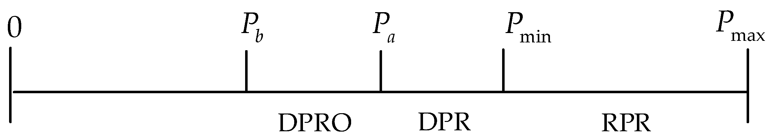
According to the operation status and energy consumption characteristics of thermal power units, the peak regulation process can be divided into three stages: regular peak regulation (RPR), deep peak regulation without oil (DPR), and deep peak regulation with oil (DPRO) [12], which are all shown in Figure 1.
In the RPR stage, the peak regulation energy consumption cost of the thermal power unit is composed of the operating coal consumption cost, which is usually calculated by coal consumption characteristics. Therefore, the operating coal consumption cost of thermal power units is as follows:
where , , and are the coefficients of unit consumption characteristic function, and is the unit price of coal in the current season.
At the stage of DPR, the depth peaking cost of thermal power units consists of two parts: operating coal consumption cost and life loss cost. At this stage, significantly suppressing the power of a thermal unit results in high thermal stresses in its rotor shaft, and the alternating high thermal stresses result in low-cycle fatigue wear and creep wear, which in turn lead to significant deformation and even the fracture of the unit, and thus reduce its service life [13]. The fatigue life of the rotor of the unit is mainly expressed by the cracking cycle [17]:
where is the cost of purchasing the unit, is the number of cycles to failure of the rotor, is the elastic modulus of the material, is the stress at the calculated point, is the fatigue strength limit of the material, and is the section shrinkage factor of the material.
At the stage of DPRO, the peaking cost, in addition to the cost of the DPR stage, also needs to take into account the cost of oil production :
where is the fuel consumption for the unit to stabilize the fuel, and is the oil price for the season.
In summary, it can be concluded that the operating costs of thermal power units in different peaking stages are different. The three-stage peaking cost of thermal units can be expressed as Equation (5).
3. Flexibility Margin of Power System
The term flexibility is defined as the ability of a power system to cope with variability and uncertainty in both generation and demand [18]. To maintain a safe and reliable power supply capability in modern power systems, the system requires that the flexibility of all types of resources be greater than the level of flexibility demand at any time. The power system flexibility margin index and its quantitative calculation method are developed in this section on the basis of flexibility supply and flexibility demand balance mechanisms.
3.1. Analysis of Flexibility Resource
In the process of operation of a power system, all adjustment methods that could cope with fluctuations and uncertainties can be flexible resources, which may be derived from the generation side, the load side, or energy storage. The flexible resources involved in this paper include thermal power units, demand response, and energy storage. The generation side is capable of adjusting the thermal unit to offer flexibility. The load side mainly improves the flexibility of the power system through demand response. Energy storage provides flexibility through the shift of power supply and demand time.
3.1.1. Flexibility of Thermal Power Units
Due to the directionality of flexibility, when load and renewable energy power fluctuations lead to power shortage or surplus in the system, the thermal unit is able to provide upward and downward adjustment capacity for the system within its output range during the dispatch period. Normally, the regulation capacity of thermal power units is . After entering the deep peaking state, the thermal power can provide greater downward-regulation flexibility for the system.
If the power of the thermal power unit at the time is , then the maximum output power of the unit, the minimum output power of the unit at the RPR stage, and the minimum stable output power at the DPRO stage are , , and ; the upward-regulation flexibility provided by the thermal power unit for the system is Equation (6); the downward-regulation flexibility that can be provided by the conventional unit is Equation (7); and the downward adjustment flexibility for the deep peaking unit is Equation (8).
where and represent the maximum upward and downward ramp rates for the unit , and is the system scheduling time scale.
3.1.2. Flexibility of Demand Response
Demand response (DR) is a form of power supply and demand interaction based on the electricity price signal or the incentive mechanism wherein the user changes the inherent power consumption mode to change the power load [19]. According to the different response modes of users, DR can be divided into two types: price-based DR and incentive-based DR. Usually, incentive-based DR can be used as a direct scheduling resource to perform joint power dispatching optimization, but the response bias of price-based DR is greatly affected by the response elastic coefficient and the excitation level, and thus, direct scheduling decisions cannot be made. Therefore, this paper mainly considered incentive-based DR.
Incentive-based DR refers to a situation where the user responds to the dispatch center interrupt load request at a specific time according to the signed contract, reduces or interrupts the power consumption, and obtains corresponding economic compensation [20]. When the system dispatcher issues an interrupt command to the user, the user should consciously respond with load reduction, and the load relationship before and after the reduction is
where and are the load demand before and after the load is reduced in period , is the number of interruptible users, is the state variable of the interruptible user in period , the value of 1 indicates that the load is in an interrupted state, the value of 0 indicates that the load is not interrupted, and is the interruptible load of the user in period .
The interruptible load can be integrated into the virtual power plant to participate in the system operation during the scheduling process. The single interruptible load can be regarded as the unit in the virtual power plant. The flexibility of the upward and downward regulation that can be provided by the interruptible load is
3.1.3. Flexibility of Energy Storage
The state of charge (SOC) of the battery energy storage system (BESS) is a parameter of great importance in the process of charging and discharging, which reflects the ratio of the remaining capacity of the BESS to the total capacity in the current period [21]. The formula is as follows:
where is the charging state of the BESS in period , is the charging and discharging efficiency of the BESS, is the maximum capacity of the BESS, is the charging and discharging power of the period BESS; when its value is greater than 0, it is the discharge power, and when it is less than 0, it is the charge power. and are the charging and discharging efficiency of the battery energy storage, respectively, is the charging and discharging efficiency of the BESS in period , the value of which is related to the charging and discharging state of the BESS, and the specific calculation method is as shown in Equation (12).
As a kind of flexible resource, the flexibility of the upward and downward regulation offered by energy storage can be controlled by the state of charge as well as by the charge and discharge strategy. The specific calculation method is as follows:
where and are the upward-regulation flexibility and the downward-regulation flexibility provided by the energy storage device, and are the maximum charging and discharging power of the energy storage device, and and are the upper and lower limits of the SOC.
3.2. Analysis of Flexibility Demand
Before a fluctuating power supply such as wind power is connected to the power grid, the uncertainty of the power system mainly comes from load changes and unexpected disturbances caused by conventional power failure. Large-scale wind power integration brings more uncertainty to the power system after it is connected to the power grid. The power system flexibility demand studied in this paper was mainly in accordance with load climbing, the inaccuracy of load, and wind power forecasting.
The demand for up or down flexibility of the system at a certain moment is mainly determined by the demand of load climbing up or down at the next time, and the prediction error level of the load and wind power. The specific mathematical expressions are as follows:
where and are the demand for upward regulation and downward regulation flexibility of the system in period , is the predicted value of the system load in period , is the predicted value of the wind power in period , and are the demand coefficients for the upward and downward adjustment due to the load prediction error, and and are the demand coefficients for the upward and downward adjustment due to the wind prediction error.
3.3. Index of Flexibility Margin
Based on the above description of system flexibility supply and demand, the power system flexibility margin indicator was defined as the difference between the sum of the system flexibility resource supply and the flexibility demand. Since the flexibility supply and demand are both directional, correspondingly, the flexibility margin also has two directions, up or down, as defined below.
where is the total upward-regulation flexibility margin of the system in period , and is the total downward-regulation flexibility margin of the system in period .
4. Optimal Scheduling Model for Multi-Energy Power Systems with Multiple Flexible Resources and Large-Scale Wind Power
4.1. Objective Function
The model established in this paper is for joint scheduling optimization of thermal units, interruptible loads, and energy storage, and aims minimize the total dispatching cost of the system, including the fuel cost of power generation, start–stop costs of thermal power units, penalty costs for wind abandonment and loss of load, and the cost of compensation for load interruption. The load interruption compensation cost refers to the economic compensation cost for the users who reduce the load, which is generally a quadratic function [22,23].
where is the number of the thermal unit; , , and are the cost coefficients of the thermal unit ; is the fuel cost for power generation; is the start–stop cost; is the on/off status of unit in period ; is the start and stop cost for thermal unit ; is the penalty cost for wind abandonment; is the cost coefficient for wind abandonment; is the abandoned wind power of the system in period ; is the penalty cost for loss of load; is the loss of load in period ; is the penalty cost coefficient for loss of load; is the cost of compensation for load interruption; and and are the quadratic coefficient and the first term coefficient of the compensation cost.
4.2. Constraints
Multi-energy power systems with large-scale wind power and multi-flexibility resources should meet the following constraints on the basis of meeting the operational constraints of conventional units.
1. Electric power balance constraint of the whole system in each period .
where is the wind power in period .
2. Minimum and maximum output constraints of conventional units in each period .
3. Minimum and maximum output constraints of the deep peaking unit in each period .
4. Battery energy storage operation constraints in each period .
where is the battery power value stored in period , is the rated power capacity for the battery energy storage, and is the limited minimum power capacity for the battery energy storage.
Equation (26) is the energy state constraint of the energy storage device, Equation (27) is the output power constraint of battery energy storage, and Equation (28) indicates that the remaining capacity of the battery energy storage needs to be consistent for starting and ending time.
5. Interruptible load constraints:
where and are the maximum and minimum interruptible power of interruptible users in period , indicates the continuous interrupted time of interruptible user in period , and are the minimum interruptible time and maximum interruptible time for the user , and is the maximum number of interrupts for the user throughout the scheduling cycle.
Equation (29) is the maximum and minimum interruptible amount constraint for each interruptible user, Equation (30) is the interruptible time constraint of the interruptible user, and Equation (31) is the maximum interruptible number constraint of the interruptible user.
4.3. Solution Methods
Considering that the operating cost of the peak regulation of a thermal unit is a nonlinear function, the quadratic programming model could not be directly solved by the CPLEX solver. Using the method described in Reference [24], the nonlinear constraint in the coal consumption cost function was converted into a linear function, where Equation (5) is rewritten as Equation (33).
Accordingly, Equation (33) linearized was equivalent to the following inequality constraint:
For the linearized model, this paper employed commercial optimization software CPLEX to solve it on the platform of MATLAB.
5. Case Study
5.1. Basic Data
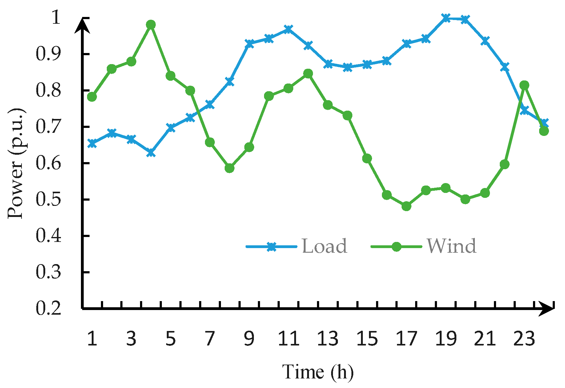
A simulation study of a modified system consisting of 26 units with 3105 MW total installed capacity and 2700 MW maximum load was carried out. The detailed data of the 26 units and the traditional load profile were obtained from Reference [25], the conventional units were peaked at 50% rated power, and two sets of 300 MW unit participated in deep peak regulation with peaking depth. A wind farm with a total capacity of 800 MW was integrated into the system; the curves of load and wind power output are shown in Figure 2. Cost coefficients for wind abandonment and loss of load were set to 100 $/MWh and 1000 $/MW [8]. Some important parameters of battery energy storage and interruptible load are listed in Table 1 [26,27]. In addition, following Reference [16], we further assumed that the parameters of the value function were , and .
5.2. Comparative Analysis of System Scheduling Results in Different Cases
In order to compare the impact of different flexible resources on the economics of wind-integrated systems and the consumption of wind power, this paper compared and analyzed the operation of the following five scheduling cases.
- Case 1:
- The thermal units are in conventional peak regulation, and there is no other flexible resources.
- Case 2:
- Two 300 MW thermal units are in deep peak regulation and there is no other flexible resources.
- Case 3:
- With the demand response resources, the thermal units are in conventional peak regulation.
- Case 4:
- With energy storage resources, the thermal units are in conventional peak regulation.
- Case 5:
- Containing energy storage and demand response resources, two 300 MW thermal units are in deep peak regulation.
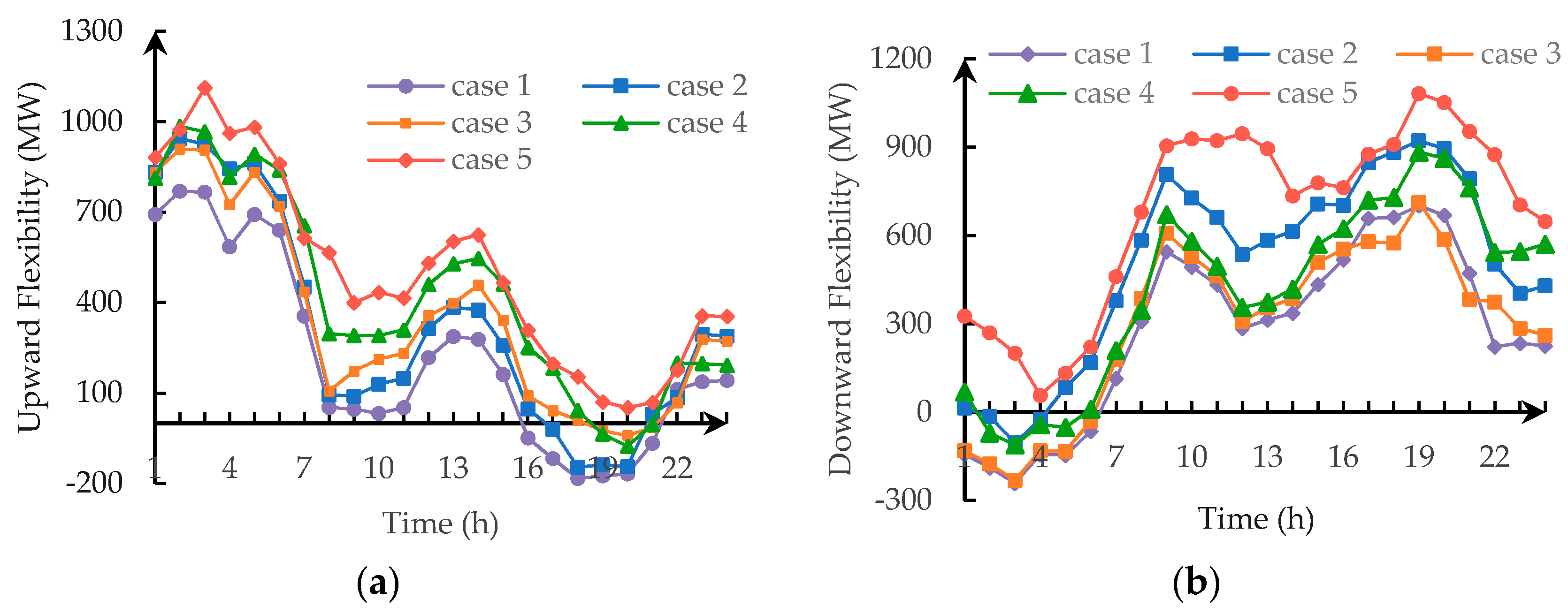
Table 2 presents the operational indicators of the system in different scheduling cases. In addition, the optimization results of the upward-regulation and downward-regulation flexibility margins of the system are illustrated in Figure 3a,b.
Note that including the three flexible resources of deep peak regulation, energy storage, and demand response could improve the economics and flexibility of the whole system. Compared with Case 1, the total dispatching costs of Case 2, Case 3, and Case 4 were reduced by 9.67%, 9.36%, and 10.09%. Additionally, it was observed that the system’s upward-regulation and downward-regulation flexibility margins were also improved, which accounts for improvement of wind power consumption.
Comparing the system flexibility margins in different scenarios in Table 1, it can be seen that Case 1 had poor system regulation performance due to the fact that only the thermal unit was in the conventional peak regulation mode, and it did not contain other flexible resources. It is worth noting that owing to lack of flexibility in the system’s upward adjustment, the value of the upward-regulation flexibility margin of the system was negative in Case 1 from 17:00 to 20:00, during which the load was at peak and the wind power was low. Additionally, when the load was low and the wind power was large from 1:00 to 6:00, the value of the downward flexibility margin of the system was also negative, due to a lack of flexibility in the system’s downward-regulation adjustment.
In Case 2, the two 300 MW units played an important role in deep peak regulation from 1:00–6:00, leading to the penalty cost of wind abandonment reducing from $138,000 to $24,000. It is worthwhile to analyze that compared with the energy storage resources, the downward adjustment space provided by the deep peak regulation of thermal unit was more sufficient, and the promotion effect on the wind power consumption was more significant. When the units were in deep peak regulation, although additional unit life loss cost and oil injection cost were added, taking measures of deep peak regulation could further improve system flexibility and reduce system start–stop cost. Furthermore, part of thermal power output was replaced with wind power, which contributed to reducing the cost of thermal power generation as well as the total scheduling cost.
In Case 3, the incentive demand response interrupted part of the load during the peak load period, which reduced the startup of the unit; meanwhile, upward-regulation standby demand of the system and penalty cost for loss of load were decreased. As for Case 4, due to the access to energy storage, the system’s chargeable and retractable operating characteristics played a prominent role in transferring wind energy abandoned from 1:00–6:00 into high-value electric energy during the peak load period, which helped to reduce the cost of generating electricity and increase the consumption of wind power in the system. At the same time, the fast response capability of the energy storage improved the adjustable capacity of the system. Therefore, the flexibility of the system’s upward and downward adjustment in Case 3 was more sufficient than that of Case 1.
For Cases 2 and 4, although the peak regulation of thermal units and energy storage enhanced the system’s downward adjustment capability, the downward adjustment capability provided by one kind of flexible resource was limited, which led to the system having a poor downward-regulation flexibility margin from 1:00–6:00. For Cases 3 and 4, the demand response and energy storage had an important impact on increasing the system’s upward adjustment capability, while there was still a certain lack of upward-regulation adjustment capability during the peak load period (19:00–21:00), and the system’s wind abandonment was also serious.
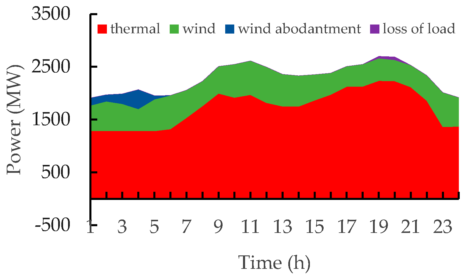
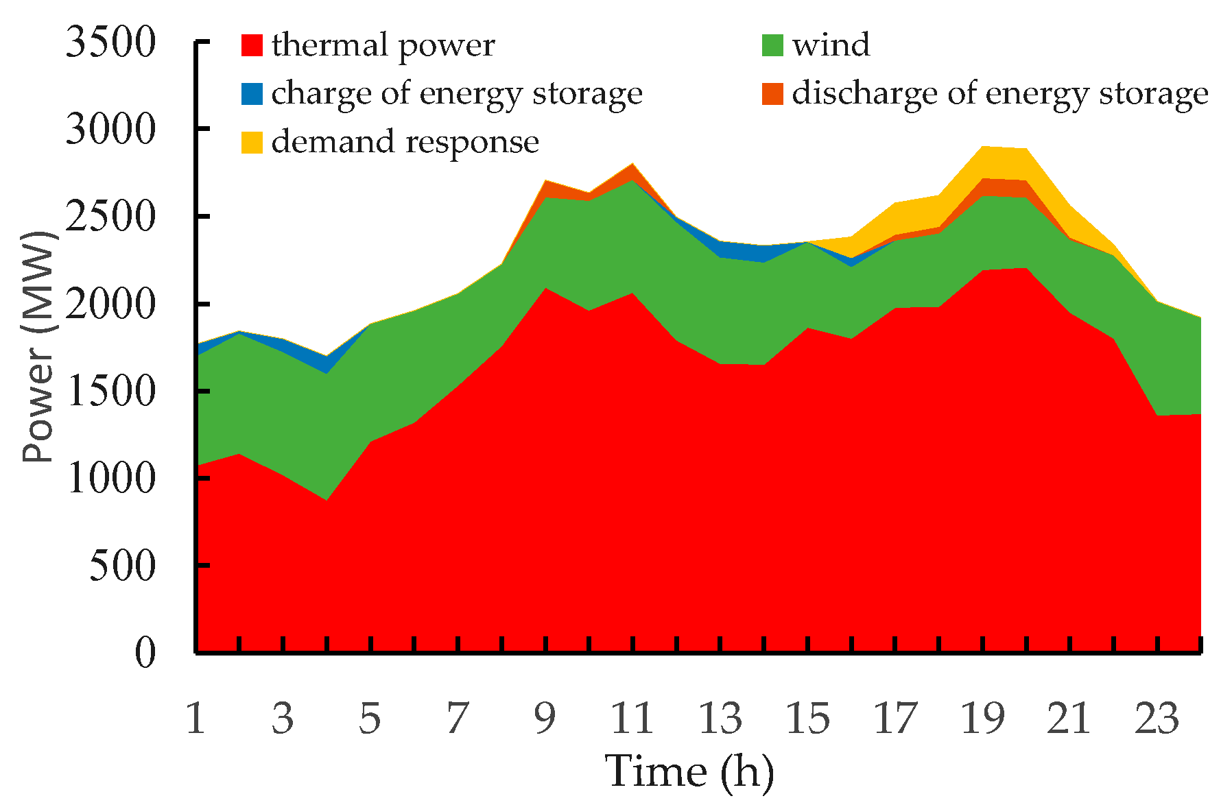
As can be seen from Figure 4 and Figure 5, in Case 5, due to the introduction of multiple flexible resources, the flexibility of the system was sufficient to respond to the flexibility demand brought by load ramping, load, and wind power prediction bias. When the load was low and the wind power was large, the thermal power unit was in deep peak regulation and the energy storage is charged, which improved the ability of the system to adapt to wind power and reduced the wind abandonment of the system. When the load was at peak and the wind power was low, part of the load was in an interrupted state and the stored energy was discharged, which relieved the load pressure at the peak time and reduced the system’s loss of load.
In conclusion, when the three kind of flexible resources work together, except for the reduction of the wind power abandonment and loss of load, the operating economy of the system in Case 5 showed the superiority over that of in other cases, and the total dispatching cost was reduced by 18.71% compared with that of Case 1. It can be concluded that the scheduling method proposed in this paper could provide a guiding direction for solving the problem of peak regulation caused by large-scale wind power integration.
5.3. Sensitivity Analysis of Wind Power Capacity
This section analyzed the system operation indicators under different wind power capacities, which are shown in Table 3.
The analysis in this section was based on the Case 5. Table 3 reveals that an increase in wind capacity led to a decreased cost of power generation. However, due to the increase of wind capacity, the flexibility demand brought by the anti-peak characteristic of wind was enhanced, which resulted in the increase of start–stop costs and deep peak regulation costs of the system. When the wind power capacity reached 1000 MW, the total dispatching cost of the system achieved the lowest level. While the wind power access capacity continued to increase to 1200 MW, the penalty cost for wind abandonment and loss of load increased greatly because of the limited regulation capacity of the system units, the insufficient capacity of energy storage equipment, and the limited demand response resources. The increasing magnitude of penalty cost for wind abandonment and loss of load was larger than the reduction of generation cost, which contributed to the increase of the total dispatching cost of the system. Therefore, the wind power consumed by the system cannot grow indefinitely, due to the limitation of capacity of flexible resources.
6. Conclusions
A model for optimizing the unit commitment, the charging/discharging profile of energy storage, and interruption plan for interruptible loads has been proposed in this paper, the objective of which is to minimize the overall cost of the power system. By means of the power system flexibility margin index, it becomes simple to evaluate the adjustment potential of various flexible resources and the flexibility of system operation.
An implementation of case studies based on a RTS96 test system showed that deep regulation of thermal units and energy storage enhanced the downward-regulation ability of the system to adapt to wind power and reduce the wind abandonment of the system; meanwhile, demand response and energy storage improved the upward-regulation ability of the system to relieve the load pressure at the peak time and decrease the system’s loss of load. Different types of flexible resources containing deep regulation of thermal units, energy storage, and demand response can not only enhance the flexibility of system operation to cope with the flexibility demand of load ramping, load, and wind power prediction bias, but can also reduce systems’ wind power abandonment rate and improve the economics of operation. In addition, the results of the examples showed that multi-type flexible resources had better regulation characteristics and operational economy than those of systems with a single flexible resource.
Author Contributions
Y.W. proposed the core idea; Q.C. developed the models, performed the simulations, and exported the results; S.L. and X.Z. helped analyze the data and edited the figures and tables; X.W. provided some important reference material. All authors discussed the results and contributed to writing this paper.
Funding
This research was funded by the National Key Research and Development Program of China grant number 2017YFB0902200, Science and Technology Project of State Grid Corporation of China grant number 5228001700CW and The National Natural Science Foundation of China grant number 51677076.
Conflicts of Interest
The authors declare no conflict of interest.
References
- Global Wind Energy Council. Global Wind Report 2017; Global Wind Energy Council: Brussels, Belgium, 2018. [Google Scholar]
- Heggarty, H.; Bourmaud, J.; Girard, R. Multi-temporal Assessment of Power System Flexibility Requirement. Appl. Energy 2019, 238, 1327–1336. [Google Scholar] [CrossRef]
- Lu, Z.X.; Li, H.B.; Qiao, Y. Flexibility Evaluation and Supply/Demand Balance Principle of Power System with High-penetration Renewable Electricity. Proc. CSEE 2017, 37, 9–20. [Google Scholar]
- Auer, H.; Haas, R. On integrating large shares of variable renewables into the electricity system. Energy 2016, 115, 1592–1601. [Google Scholar] [CrossRef]
- Lund, P.D.; Lindgren, J.; Mikkola, J. Review of energy system flexibility measures to enable high levels of variable renewable electricity. Renew. Sustain. Energy Rev. 2015, 45, 785–807. [Google Scholar] [CrossRef] [Green Version]
- Mathiesen, B.V.; Lund, H.; Connolly, D. Smart Energy Systems for coherent 100% renewable energy and transport solutions. Appl. Energy 2015, 145, 139–154. [Google Scholar] [CrossRef]
- Dui, X.; Zhu, G.; Yao, L. Two-Stage Optimization of Battery Energy Storage Capacity to Decrease Wind Power Curtailment in Grid-Connected Wind Farms. IEEE Trans. Power Syst. 2018, 33, 3296–3305. [Google Scholar] [CrossRef]
- Yang, T.M.; Lou, S.H.; Zhang, X.C. Coordinated optimal operation of hybrid energy storage in power system accommodated high penetration of wind power. In Proceedings of the 2015 5th International Conference on Electric Utility Deregulation and Restructuring and Power Technologies (DRPT), Changsha, China, 26–29 November 2015. [Google Scholar]
- Hajibandeh, N.; Shafie-khah, M.; Gerardo, J. A heuristic multi-objective multi-criteria demand response planning in a system with high penetration of wind power generators. Appl. Energy 2018, 212, 721–732. [Google Scholar] [CrossRef]
- Gao, J.W.; Ma, Z.Y.; Guo, F.J. The influence of demand response on wind-integrated power system considering participation of the demand side. Energy 2019, 178, 723–738. [Google Scholar] [CrossRef]
- Liu, X.C.; Wang, P.P.; Li, Y. Stochastic Unit Commitment Model for High Wind Power Integration Considering Demand Side Resources. Proc. CSEE 2015, 35, 3714–3723. [Google Scholar]
- Lin, L.; Tian, X.Y. Analysis of deep peak regulation and its benefit of thermal units in power system with large scale wind power integrated. Power Syst. Technol. 2017, 41, 2255–2263. [Google Scholar]
- Yang, Y.; Qin, C.; Zeng, Y. Interval Optimization-Based Unit Commitment for Deep Peak Regulation of Thermal Units. Energies 2019, 12, 922. [Google Scholar] [CrossRef]
- Deng, T.T.; Lou, S.H.; Tian, X. Optimal Dispatch of Power System Integrated with Wind Power Considering Demand Response and Deep Peak Regulation of Thermal Power Units. Autom. Electr. Power Syst. 2019, 43, 24–41. [Google Scholar]
- Tan, Z.F.; Ju, L.W.; Li, H.H. A two-stage scheduling optimization model and solution algorithm for wind power and energy storage system considering uncertainty and demand response. Int. J. Electr. Power Energy Syst. 2014, 63, 1057–1069. [Google Scholar] [CrossRef]
- Su, C.G.; Shen, J.J.; Wang, P.L.; Zhou, L.G.; Cheng, C.T. Multi-source coordinated scheduling method for wind power system based on power supply flexibility margin. Autom. Electr. Power Syst. 2018, 42, 111–122. [Google Scholar]
- Xie, T.; Lv, K.; Huang, J.S. Study on the thermodynamic characteristic of generalized regenerative system used for deep peak load regulating operation. Therm. Power Gener. 2018, 5, 71–76. [Google Scholar]
- Ma, J.; Silva, V.; Belhomme, R. Evaluating and Planning Flexibility in Sustainable Power Systems. IEEE Trans. Sustain. Energy 2013, 4, 200–209. [Google Scholar] [CrossRef]
- Lynch, M.; Nolan, S.; Devine, M.T. The impacts of demand response participation in capacity markets. Appl. Energy 2019, 250, 444–451. [Google Scholar] [CrossRef] [Green Version]
- Logenthiran, T.; Srinivasan, D.; Shun, T.Z. Demand Side Management in Smart Grid Using Heuristic Optimization. IEEE Trans Smart Grid 2012, 3, 1244–1252. [Google Scholar] [CrossRef]
- Lou, S.H.; Wu, Y.W.; Cui, Y.Z. A Battery Energy Storage Strategy for Short-Term Wind Power Power Fluctuation. Autom. Electr. Power Syst. 2014, 38, 17–22. [Google Scholar]
- Yang, Y.; Chen, Y.Y.; Zhang, W. Power Market Model Considering Distributed Generation and Incom-plete Information Interruptible Load Selection. Proc. CSEE 2011, 31, 15–24. [Google Scholar]
- Jian, X.H.; Zhang, L.; Miao, X.F. Designing Interruptible Load Management Scheme Based on Customer Performance Using Mechanism Design Theory. Electr. Power Energy Syst. 2018, 95, 476–489. [Google Scholar] [CrossRef]
- Zhang, N.; Kang, C.; Xia, Q. A Convex Model of Risk-Based Unit Commitment for Day-Ahead Market Clearing Considering Wind Power Uncertainty. IEEE Trans. Power Syst. 2014, 30, 1582–1592. [Google Scholar] [CrossRef]
- Grigg, C.; Wong, P.; Albrecht, P.; Allan, R.; Bhavaraju, M.; Billinton, R.; Chen, Q.; Fong, C.; Haddad, S.; Kuruganty, S.; et al. The IEEE reliability test system-1996. IEEE Trans. Power Syst. 1999, 14, 1010–1018. [Google Scholar] [CrossRef]
- Niu, W.J.; Li, Y.; Wang, W. Modeling of Demand Response Virtual Power Plant Considering Uncertainty. Proc. CSEE 2014, 34, 3630–3637. [Google Scholar]
- Lu, Z.G.; Guo, K.; Yan, G.H. Optimized Scheduling of Wind Power System Based on Demand Response for Virtual Machines and Carbon Trading. Autom. Electr. Power Syst. 2017, 41, 58–65. [Google Scholar]
Figure 1.
Three-stage peaking regulation process of thermal power unit: is the maximum output of the unit, is the minimum technical capacity of the unit at the stage of regular peak regulation (RPR), is the minimum rated capacity of the unit at the deep peak regulation without oil (DPR) stage, and is the minimum stable output at the deep peak regulation with oil (DPRO) stage.

Figure 2.
Load and wind power scenarios.

Figure 3.
Different cases of flexibility margin: (a) upward-regulation flexibility of system in different cases; (b) downward-regulation flexibility of system in different cases.
Figure 3.
Different cases of flexibility margin: (a) upward-regulation flexibility of system in different cases; (b) downward-regulation flexibility of system in different cases.

Figure 4.
Scheduling plan of Case 1.

Figure 5.
Scheduling plan of Case 5.


Table 1.
Relevant parameters of energy storage and interruptible load.
| Parameters | Values |
|---|---|
| Capacity of energy storage (MWh) | 400 |
| Rated charging/discharging power (MW) | 100 |
| Charging and discharging efficiency | 90 |
| Capacity of each interruptible user (MW) | 60 |
| Number of interruptible users | 3 |
| Maximum interruptible time (h) | 6 |
| Minimum interruptible time (h) | 3 |
| Quadratic coefficient of compensation cost | 0.4 |
| First term coefficient of compensation cost | 25 |
Table 2.
Indicators under different cases.
| Cost | Case 1 | Case 2 | Case 3 | Case 4 | Case 5 |
|---|---|---|---|---|---|
| Total dispatching cost (104 $) | 287.5 | 259.7 | 260.6 | 258.1 | 233.7 |
| Fuel cost (104 $) | 248.5 | 235.9 | 238.7 | 225.4 | 217.2 |
| Start–stop costs (104 $) | 15.6 | 12.6 | 13.4 | 14.8 | 11.2 |
| Penalty cost for wind abandonment (104 $) | 13.8 | 2.4 | 6.4 | 12.6 | 0 |
| Penalty cost for loss of load (104 $) | 9.6 | 8.8 | 2.1 | 0 | 0 |
| Compensation for load interruption (104 $) | 0 | 0 | 0 | 5.3 | 5.3 |
| Cost for peak regulation (104 $) | 0 | 4.4 | 0 | 0 | 2.3 |
Table 3.
Operational indicators under different wind power capacity.
| Cost | 400 (MW) | 600 (MW) | 800 (MW) | 1000 (MW) | 1200 (MW) |
|---|---|---|---|---|---|
| Total dispatching cost (104 $) | 261.8 | 248.2 | 233.7 | 223.6 | 227.0 |
| Fuel cost (104 $) | 247.5 | 232.3 | 217.2 | 203.7 | 195.1 |
| Start–stop costs (104 $) | 9.8 | 10.6 | 11.2 | 12.2 | 13.6 |
| Penalty cost for wind abandonment (104 $) | 0 | 0 | 0 | 2.4 | 9.8 |
| Penalty cost for loss of load (104 $) | 0 | 0 | 0 | 0 | 3.2 |
| Compensation for load interruption (104 $) | 4.5 | 5.3 | 5.3 | 5.3 | 5.3 |
| Cost for peak regulation (104 $) | 0.6 | 1.7 | 2.3 | 3.8 | 5.6 |
© 2019 by the authors. Licensee MDPI, Basel, Switzerland. This article is an open access article distributed under the terms and conditions of the Creative Commons Attribution (CC BY) license (http://creativecommons.org/licenses/by/4.0/).
Share and Cite
MDPI and ACS Style
Che, Q.; Lou, S.; Wu, Y.; Zhang, X.; Wang, X. Optimal Scheduling of a Multi-Energy Power System with Multiple Flexible Resources and Large-Scale Wind Power. Energies 2019, 12, 3566. https://doi.org/10.3390/en12183566
AMA Style
Che Q, Lou S, Wu Y, Zhang X, Wang X. Optimal Scheduling of a Multi-Energy Power System with Multiple Flexible Resources and Large-Scale Wind Power. Energies. 2019; 12(18):3566. https://doi.org/10.3390/en12183566
Chicago/Turabian StyleChe, Quanhui, Suhua Lou, Yaowu Wu, Xiangcheng Zhang, and Xuebin Wang. 2019. "Optimal Scheduling of a Multi-Energy Power System with Multiple Flexible Resources and Large-Scale Wind Power" Energies 12, no. 18: 3566. https://doi.org/10.3390/en12183566
Note that from the first issue of 2016, this journal uses article numbers instead of page numbers. See further details here.