On Optimal Battery Sizing for Households Participating in Demand-Side Management Schemes


1
School of Computer Science & Mathematics at Kingston University London, Kingston upon Thames KT1 2EE, UK
2
Iberdrola Innovation Middle East, Qatar Science & Technology Park, Doha 210177, Qatar
3
Division of Engineering Management & Decision Sciences, College of Science and Engineering, Hamad Bin Khalifa University, Doha 34110, Qatar
*
Author to whom correspondence should be addressed.
Energies 2019, 12(18), 3419; https://doi.org/10.3390/en12183419
Submission received: 25 July 2019
/
Revised: 20 August 2019
/
Accepted: 22 August 2019
/
Published: 5 September 2019
(This article belongs to the Section D: Energy Storage and Application)
Abstract
:The smart grid with its two-way communication and bi-directional power layers is a cornerstone in the combat against global warming. It allows for the large-scale adoption of distributed (individually-owned) renewable energy resources such as solar photovoltaic systems. Their intermittency poses a threat to the stability of the grid, which can be addressed by the introduction of energy storage systems. Determining the optimal capacity of a battery has been an active area of research in recent years. In this research, an in-depth analysis of the relation between optimal capacity and demand and generation patterns is performed for households taking part in a community-wide demand-side management scheme. The scheme is based on a non-cooperative dynamic game approach in which participants compete for the lowest electricity bill by scheduling their energy storage systems. The results are evaluated based on self-consumption, the peak-to-average ratio of the aggregated load and potential cost reductions. Furthermore, the difference between individually-owned batteries and a centralised community energy storage system serving the whole community is investigated.
1. Introduction
Global average temperatures are rising dramatically (2016 being the warmest year ever recorded [1]), causing a noticeable increase in natural disasters and environmental issues [2]. Thus, it is imperative to investigate approaches that reduce greenhouse gas emissions and slow down climate change. Instead of burning fossil fuels to satisfy our energy needs, humans should make use of renewable energy resources such as solar and wind, which have a smaller carbon footprint. In order to guarantee a stable power grid, demand and generation have to be balanced at all times. This makes the integration of renewable resources a challenging task due to their intermittent nature. The advent of the smart grid, a technologically-advanced power grid, is a possible solution to this problem. It combines the legacy power grid with a communication layer, effectively connecting all the grid participants. Through this additional infrastructure, energy consumption can be managed.
More specifically, in this research, the functionality of exchanging data between individual households is being used to schedule energy storage installations such that the grid stability is guaranteed even though a considerable amount of demand is served from solar power generation facilities. A key element to achieve a high self-consumption rate of solar energy, i.e., the ratio between the consumed solar energy to the actual demand, is the utilisation of energy storage. Various research studies are concerned with energy storage management [3,4,5,6,7,8].
Luthander et al. [6] presented a case study of 21 Swedish households with a focus on comparing individually-owned batteries to a centralised storage solution. In order to reach a certain level of self-consumption, the centralised storage capacity was considerably smaller than the aggregated capacity of individually-owned batteries. The study in [7] was concerned with optimising the usage of a given photovoltaic-battery system. It investigated a number of different optimisation objectives and showed how these affect the eventual charging patterns of a household for two exemplary days. In contrast to their approach, the work in [8] made use of a game-theoretic approach in which households schedule their individually-owned batteries with the goal to minimise their respective electricity bills. They performed simulations over the period of an entire year to allow for statistical analysis of the results. One interesting question is: What is the optimal capacity of a battery? [9,10,11]. The work in [11] focused on the influence of different tariff schemes on the optimal battery size, whereas [10] developed a decision-making tool that supports users that are investing in photovoltaic and battery systems. Recently, Huang et al. [9] developed an algorithm to determine the optimal size of a battery with respect to the achievable self-consumption. This research builds on their approach and develops a deeper understanding of the relation between demand and generation patterns and the optimal battery capacity. In particular, we study two different demand-side management schemes. Within the first one, “Game-Theoretic Scheduling” (GTS), the households have the single goal of minimising their individual electricity bills (cf. [8]). The second scheme considers an additional preference of increasing the respective self-consumption of the household and is called “Game-Theoretic Scheduling With Constraint” (GTSWC) throughout the manuscript.
The main contributions of this research are as follows:
- (1)
- Based on seasonal and yearly simulations of households with real consumption and generation data, this research provides an in-depth insight into how optimal sizing of batteries depends not only on aggregated statistics, but also on the specific temporal patterns that characterise individual households.
- (2)
- Two different battery scheduling algorithms, i.e., GTS and GTSWC, are compared in terms of three metrics: (i) self-consumption of solar energy, (ii) the peak-to-average ratio of the aggregated load as an indicator for grid stability and (iii) potential cost reductions due to the introduction of electricity storage systems.
- (3)
- This research compares the optimal sizing for a centralised storage facility with individually-owned batteries and analyses their effect on the same metrics as mentioned above.
2. Optimal Battery Sizing Results
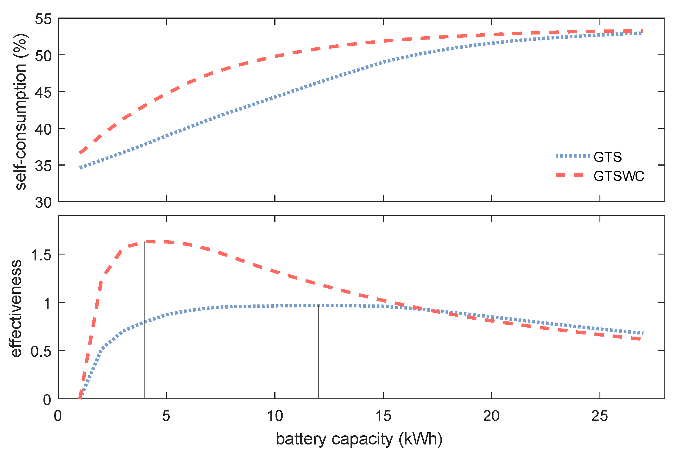
In order to determine the optimal battery size, the process described in [9] has been followed. To do so, simulations were performed with different battery sizes for each household (per season and yearly) using both scheduling approaches to be introduced in Section 4.4. Battery capacities were in the range between 1.0 kWh and 27.0 kWh. The upper limit would equal an installation of two Tesla Powerwall2 batteries [12]. For each set of parameters, the “effectiveness” of the electricity storage was computed. The effectiveness is defined by the notion of how much the self-consumption of a household is increased per kWh of installed capacity:
where is the self-consumption achieved by utilising a storage of size n kWh. The maximum of this effectiveness is the sought-after optimal battery size. An example for these steps is shown in Figure 1 for a randomly-selected house and season.
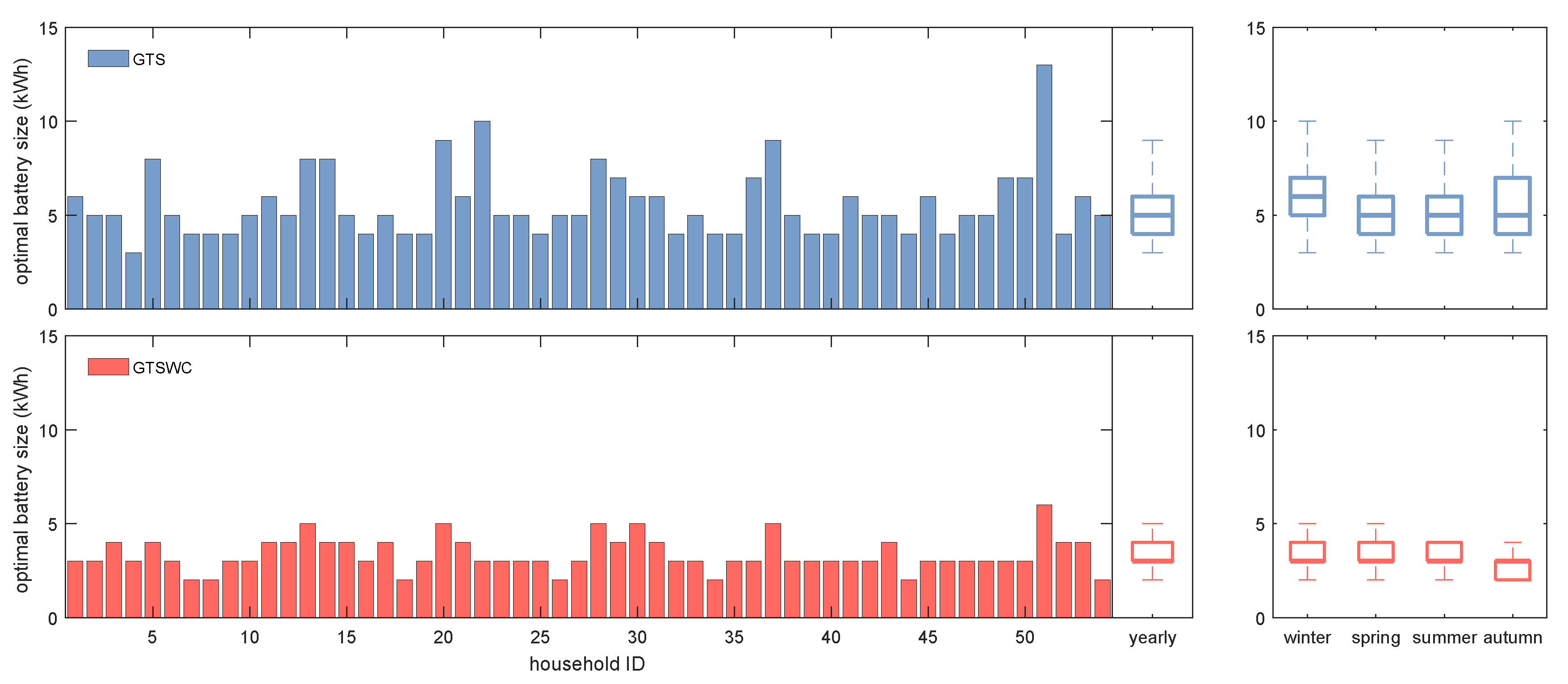
The optimal battery size for each player over the course of an entire year for the two approaches (game-theoretic scheduling with and without self-consumption constraint, cf. Section 4.4) is shown in Figure 2. Furthermore, Figure 2 also reports the average results per season over all 54 investigated households.
Overall, the optimal size for the GTSWC scenario did not exceed the GTS optimal battery size for any player and season. Household 4 showed the smallest difference between the two scenarios. All the capacities were the same except for summer, where they differed by 1 kWh. The largest difference between the optimal battery size as determined for the two approaches of a particular season was found in Household 14 (summer). Here, the difference was 8 kWh (cf. Figure 1). The largest difference between the optimal battery size for two seasons and the same approach was seen in Household 52 (winter: 11 kWh, summer: 3 kWh). In Section 3, these households are investigated in particular to understand how their battery usage patterns lead to the respective results.
2.1. Self-Consumption
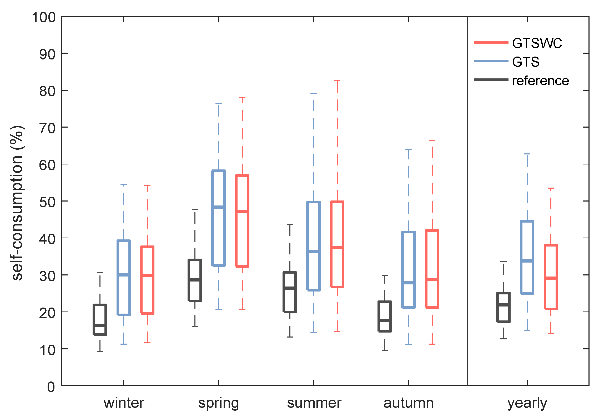
The solar PV self-consumption rate of a household is defined as the ratio between the solar energy being used and its demand. This includes a direct part, which is consumed immediately, and an indirect part used to charge the battery when the PV system generation exceeds the local demand. In the following, the increase in self-consumption due to the introduction of an optimally-sized battery for both the GTS and GTSWC scenario is analysed. The seasonal results for the self-consumption can be found in Figure 3. Explicit improvements are reported in Table 1.
It becomes clear that even with different optimal battery sizes for the GTS and GTSWC approaches, the median improvement in self-consumption is similar. The result was to be expected as the additional constraint in GTSWC was particularly designed to place further emphasis on the increase of self-consumption. The spread around the median self-consumption approximately doubled when comparing the results with the reference case in which no batteries were present. This is due to the fact that some households benefit more than others from the introduction of a battery. There are many factors that play a role in this such as the aggregated solar production, the aggregated demand and, also, the temporal patterns of production and demand. For example: Household 14 improved its self-consumption by during the summer, while Household 26 (with similar aggregated consumption and PV peak production) improved its self-consumption by . Household 13, which had less aggregated demand than the two houses mentioned before and higher aggregated solar production, improved its self-consumption by . A more detailed analysis of these households and how these differences are related to their demand patterns will be analysed in Section 3. In general, households that gain considerably with GTS also do so with GTSWC and vice versa. The average absolute difference of the self-consumption improvements between GTS and GTSWC for each household individually was <.
2.2. PAR Values
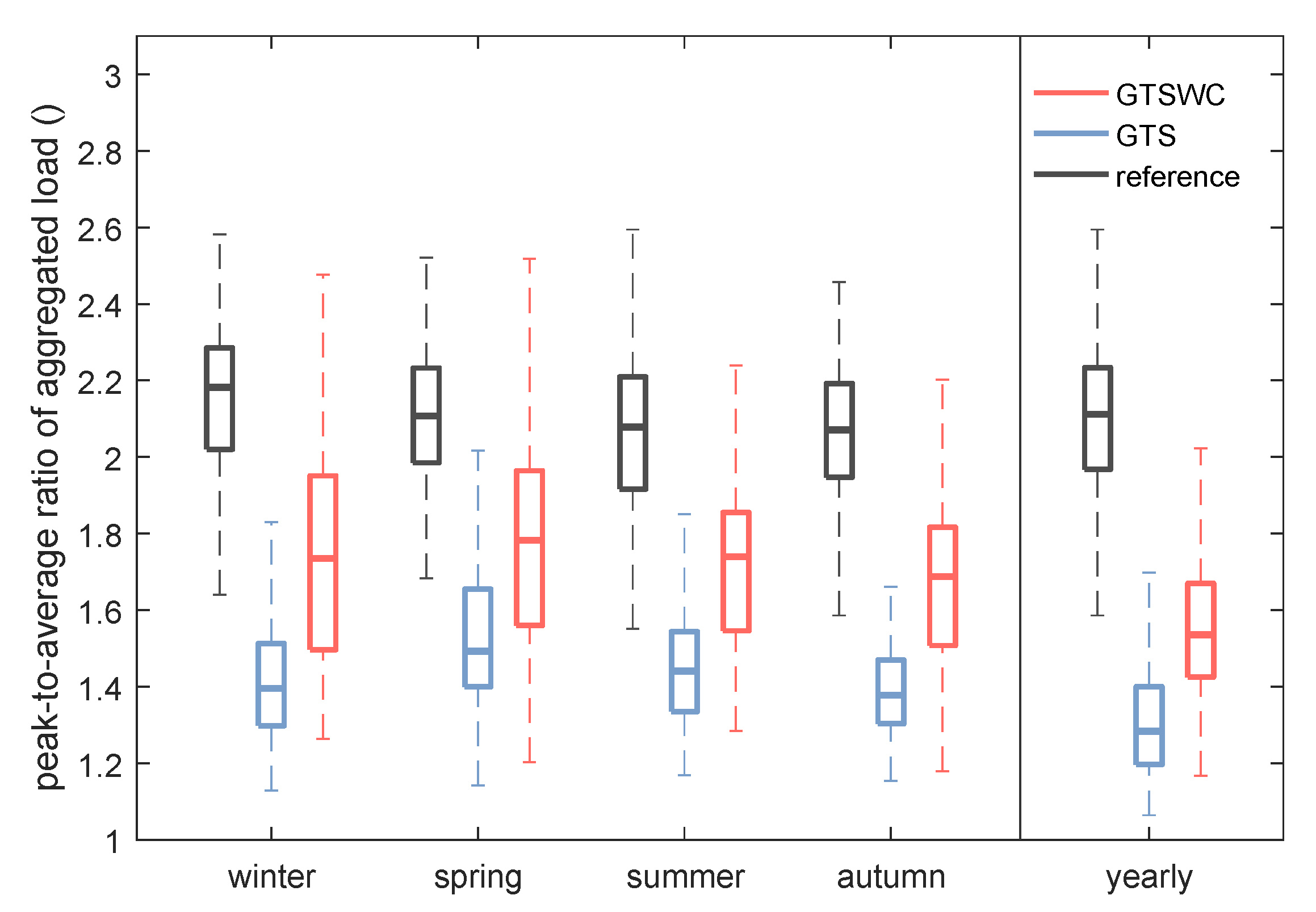
The Peak-to-Average Ratio (PAR) of the aggregated load (7) is an indicator of the stability of the grid [13]. A value close to 1.0, i.e., a flat load profile, is preferred by a utility company, as this allows them to save investment costs for fast-ramping energy production installations. PAR values are calculated for a period of one day. A statistical analysis for the 90 days that comprise each season is shown in Figure 4.
Overall, considerable improvements of the PAR value were achieved. The GTS approach led to better PAR reductions than the GTSWC approach in both the median values and also the smaller spread around these.
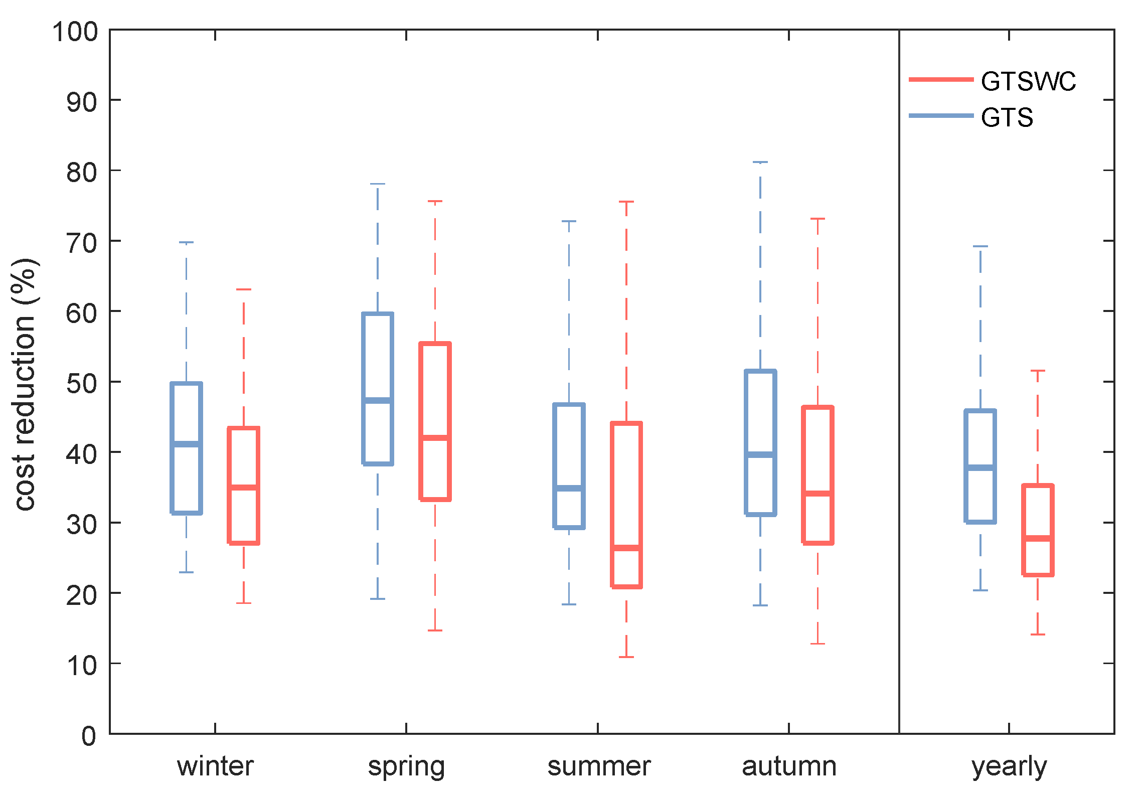
2.3. Cost Reduction
As will be seen in Section 4.3, the cost function (5) depends on the aggregated load. Thus, the price per unit of electricity changes for each half-hour interval. When calculating the overall bill for each household with and without battery, it can be observed that it is decreasing in both approaches. The relative cost reduction of the electricity bill due to the introduction of an optimally-sized battery is shown in Figure 5.
Overall, the introduction of energy storage led to a considerable amount of savings from the electricity bill in both cases (GTS and GTSWC). The increase of self-consumption can directly be translated into a decrease of energy requested from the grid, which in turn decreases the bill. As seen in the previous section (cf. Section 2.1), the achieved improvements in self-consumption were similar for the two approaches. This means this fact alone cannot explain the higher savings from GTS compared to GTSWC. The second factor that played a role was the more effective PAR reduction observed for the GTS approach (cf. Section 2.2). Due to the quadratic relation between the aggregated load and the price per unit of electricity, consumption during peak times is billed highly. The spread around the median values for both approaches was similar.
2.4. Centralised vs. Decentralised Storage Systems
In all the previous simulations, each household was in possession of an individual battery of different sizes. Within this section, a scenario that has a single battery to serve the community is investigated. For a reasonable comparison, the efficiency of the battery and the DC/AC power electronics converter equal the values used before. Furthermore, the maximal charging and discharging rates were scaled up by the number of households. Firstly, full-year simulations with battery sizes varying between 10 kWh and 370 kWh were performed. Following the optimal sizing procedure by [9], the optimal battery capacity for both the GTS and GTSWC approach were calculated to be 270 kWh and 90 kWh, respectively. For these optimal sizes, the self-consumption, the PAR of the aggregated load of all households and the cost reduction according to the pricing function (6) were analysed. The results are shown together with the respective results from yearly simulations of individually-owned batteries in Figure 6.
The centralised optimal battery sizes were approximately and smaller than the aggregated capacities of the decentralised batteries for the GTS and GTSWC approaches, respectively. This is in agreement with a previous study reported by Luthander et al. [6]. In Section 3, we discuss that in case of asynchronous demand and generation profiles, a large battery is most beneficial, while in the opposite case, a small battery is sufficient. When looking at the centralised battery, note that it is scheduled according to the aggregated demand and generation of all the households. An averaging effect for the demand profiles occurred, which made the asynchronous case less likely and eventually led to a smaller optimal storage capacity. The PV self-consumption reached a comparable level to the decentralised simulations. Compared to the median self-consumption of all the households, a scenario with a centralised battery improved the self-consumption by approximately for both the GTS and GTSWC approaches. When analysing the daily PAR values, it became clear that the community batteries performed worse both in terms of the achieved median values and also the spread around them. From the utility companies’ perspective, this is an unfavourable result. Their most desirable objective is to reduce the PAR value, as it guarantees grid stability and financial benefits in the long run.
The right-most panel in Figure 6 shows the results for the cost reduction for both approaches comparing the centralised and decentralised neighbourhoods. For the GTS approach, the centralised community achieved an approximately higher cost reduction, while for the GTSWC approach, the cost reduction was reduced by approximately compared to the median cost reduction of all the households with individually-owned batteries. Both results for the centralised battery were within the interquartile range of the respective analysis for the decentralised system. Please note that these cost reductions refer to the operational costs. To understand the complete picture, we also have to take into account the capital costs of the equipment. From [14], it can be inferred that the residential lithium-ion storage systems cost approximately 2.6-times more per kilowatt-hour compared to the utility-scale system. These costs were not taken into account when scheduling the batteries.
3. Discussion
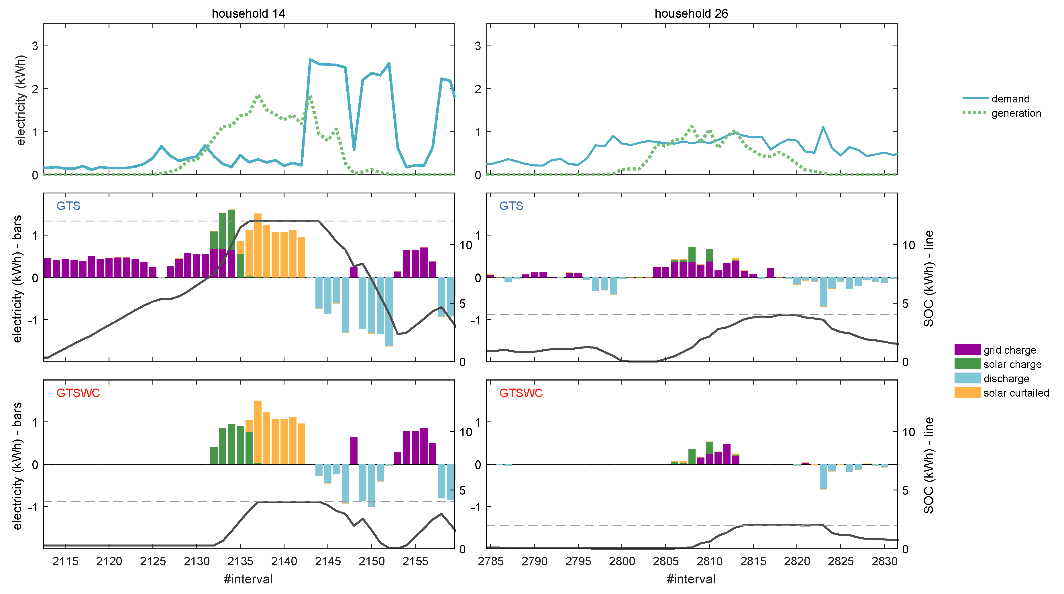
While the aggregated demand of a household and the size of their installed solar panel can give a rough estimate for the optimal battery size, it remains important to look at the actual demand and generation patterns. In Section 2.1, it was visible that two households with similar aggregated demand and potential peak PV output benefited differently from their storage installation. In order to understand this difference, Figure 7 shows the demand and generation profile for a randomly-chosen day together with the detailed battery usage for these two households.
The demand of Household 14 was low during the time when solar was available and peaked shortly afterwards, whereas the demand of Household 26 was rather evenly distributed throughout the day. Household 26 is a prime example of a user that had a high percentage of non-curtailed solar energy even without a battery installation and could not gain much through the utilisation of storage. Consequently, the optimal battery sizing algorithm determined a below-average optimal storage capacity for this household. In contrast to this, the battery of Household 14 was optimally sized at an above-average capacity. Without storage, much of the solar energy was curtailed due to the lack of demand at the particular time of generation. Since there was a peak in demand in the later hours, the self-consumption could be increased due to the storage capability.
The left-hand plots in Figure 7 also give insight into the differences between the GTS and GTSWC approaches. During the fist half of the day, the GTS algorithm charged the battery from the grid, whereas the GTSWC anticipated the solar generation and thus restricted charging from the grid. The first two peaks in demand (cf. between Intervals 2144 and 2152) can then be met by previously saved electricity. In anticipation of another peak in demand at the end of the day, both algorithms charged the battery and were able to flatten the load curve considerably. It became clear that because no more solar production was to be expected during this time, there were no constraints on charging the battery from the grid, and both algorithms behaved similarly.
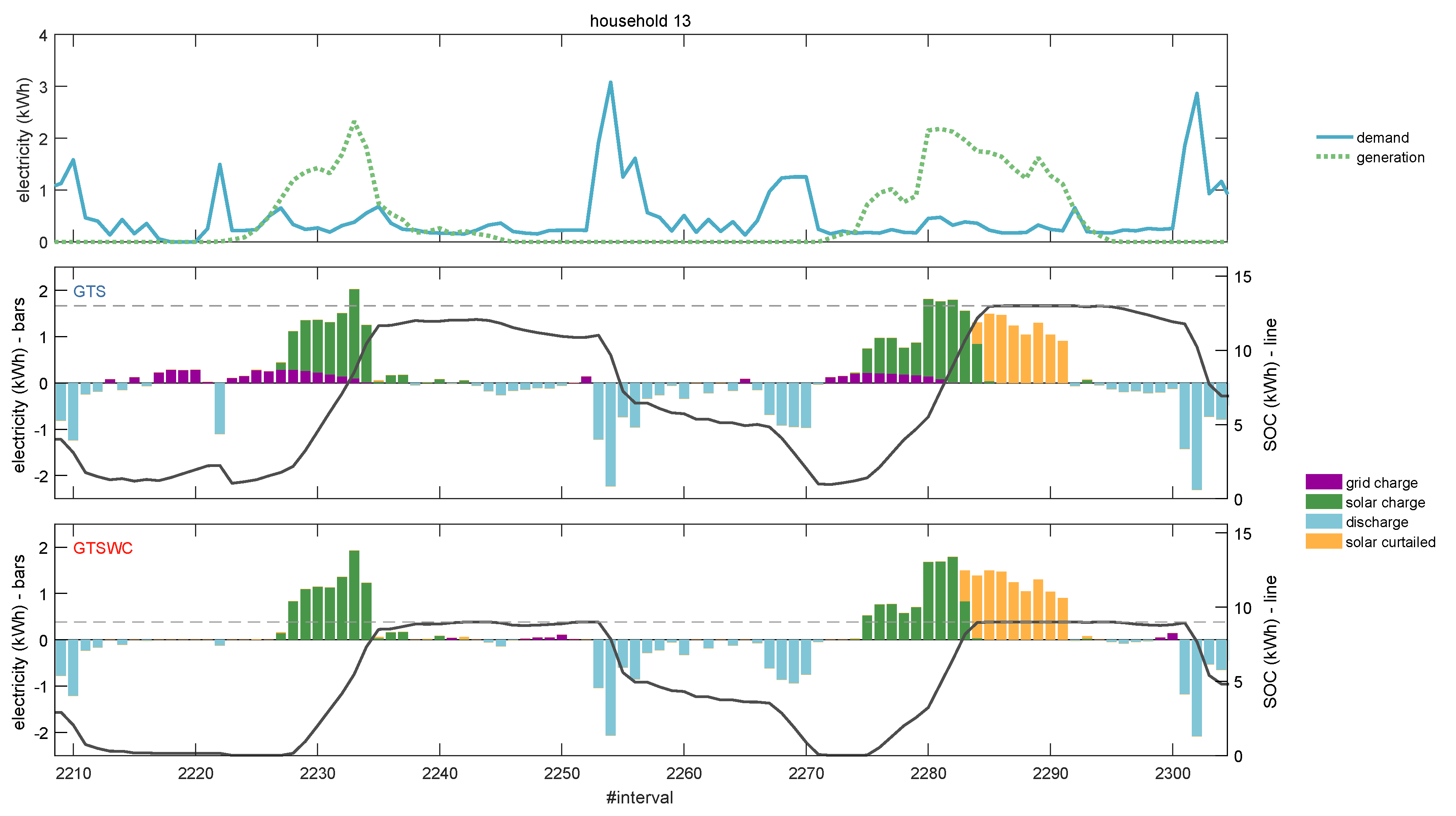
Figure 8 shows the demand and generation pattern together with the battery usage for two consecutive days of Household 13. This household was chosen as it had the highest benefit during this particular season from installing an optimal battery size. A similar profile for the demand and generation as seen for Household 14 in Figure 7 can be observed. The even higher improvement in self-consumption for this case stemmed from the more pronounced asynchronisation between solar generation and actual demand. Furthermore, this household was equipped with a bigger solar panel.
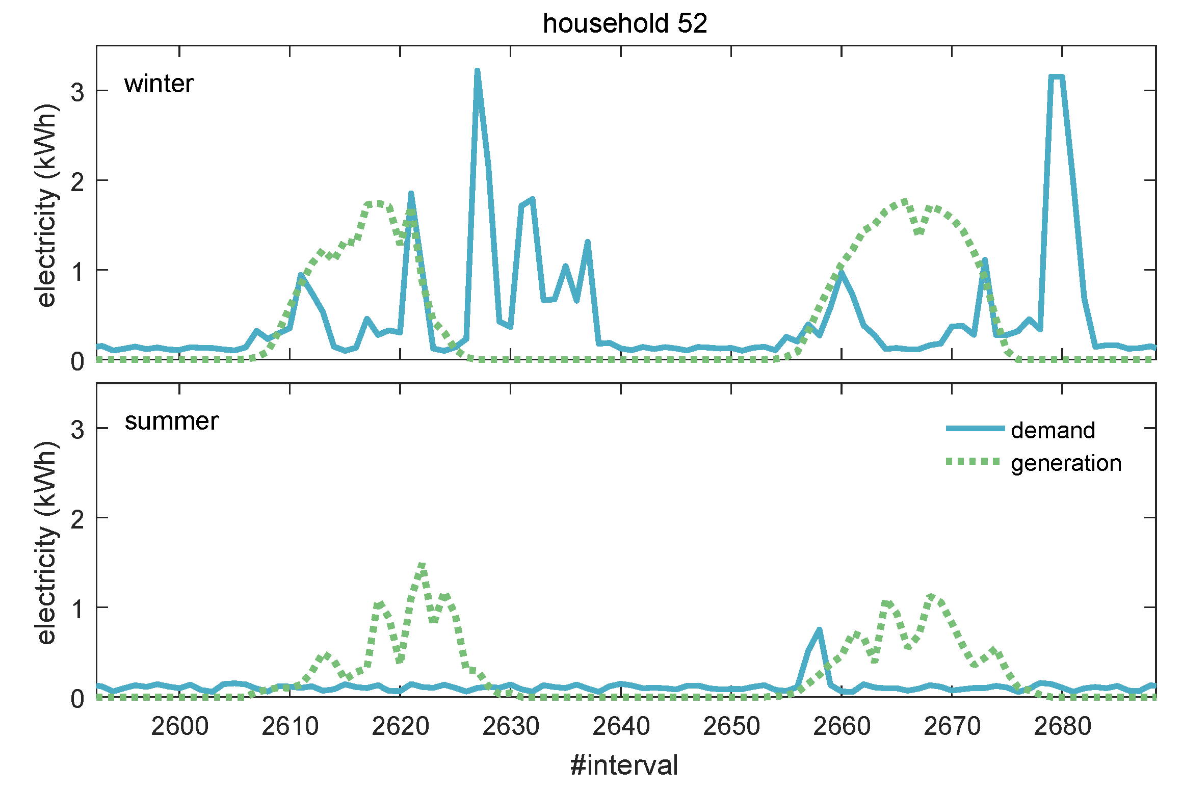
This section was concluded by analysing the demand and generation profile (Figure 9) for the household that showed the biggest difference in optimal battery size between two seasons, i.e., Household 52. For winter 2010, the optimal capacity was determined to be 11 kWh, while in summer 2011 it was 3 kWh.
4. Materials and Methods
4.1. Neighbourhood
Consider a neighbourhood of M households that is modelled as a set . Each of the households is equipped with a smart meter, an individually-owned battery and a photovoltaic (PV) system that converts solar energy into electricity. The smart meters have the capability to measure consumption and generation data over equidistant time intervals . A day is split into T intervals. Furthermore, the smart meters are able to exchange data through wireless communications. The cyber security aspects of these communication channels are an important field of research and beyond the scope of this manuscript.
4.2. Households
A detailed battery model was employed. It included the charging and discharging efficiency () of the storage device, self-discharging at a rate of in case the battery was idle and also limits on how much can be charged or discharged () during a particular interval . Furthermore, the conversion efficiency of the DC/AC power electronics converter was considered. The main equations characterising the battery model were as follows, and more details are presented in [8]:
where SOC is the State-Of-Charge of the battery, and are the charging and discharging amount in interval t, respectively, and and give the lower and upper bound of the SOC.
Each household was equipped with a solar PV system for local consumption. The PV systems varied in size according to the dataset described in Section 4.5. The solar energy generated locally was always taken into account before making a scheduling decision for a specific interval t. This means that if available, the energy from the PV system was used to fulfil the demand of a household. Furthermore, if the solar PV generation exceeded the demand, it was stored in the local battery (if possible). Note that charging the battery from the solar PV system did not require DC/AC conversion, whereas it needed to be converted to AC before it was used to fulfil demand.
Therefore, the net-demand of a household at time interval can be written as:
Then, the load on the electricity grid, i.e., the amount of electricity that is provided by the utility company, can be written as:
where represents the battery activity, i.e., or , for household .
4.3. Utility Company
All the community households were supplied by one network distribution company, which incentivised each household individually to reduce their energy consumption during peak hours. A billing strategy that calculates a unit energy price per interval t based on the aggregated load of all customers is given by:
where is the aggregated load of all users at interval t and , are constants. As a consequence, the energy bill for a particular day of an individual household can be calculated as:
4.4. Game Scheduling and Self-Consumption Constraint
The batteries of the households were scheduled based on a dynamic game, which was played between the individual households. The objective of the players/households was to minimise their individual electricity bill (6). They acted rationally and in a selfish manner. In the following section, two approaches are differentiated. The first approach is identical to the one proposed by [8] and is called “Game-Theoretic Scheduling” (GTS). The game was played for an upcoming day based on forecasts for demand and generation.
The second approach introduced an additional constraint to the GTS. Whenever the renewable PV-generated energy was expected to be higher than the demand for an upcoming interval, charging the battery from the grid was prohibited. The idea behind this was to maximise the self-consumption rate of the PV system. This approach is referred to as “Game-Theoretic Scheduling With Constraint” (GTSWC).
4.5. Data, Simulation Details and Metrics
For all the following simulations, the real-world “Ausgrid” dataset [15] was used. This dataset was collected half hourly, i.e., intervals, from 300 individual homes in the Ausgrid’s electricity network over three years (2010–2013). The respective electricity network was located in the state of New South Wales. This means we could regard them as being located close to each other and did not expect considerable differences in solar radiation and temperature. All of the homes were equipped with solar PV systems between 1.05 kWp and 9.99 kWp. The period between July 2010 and June 2011 was split into four seasons as shown in Table 2.
This was done such that each individual season spanned exactly 90 days. A clean version of the Ausgrid dataset, which contained households, was considered in this research. Please refer to [16] (Chapter 2) and [17] for a thorough analysis of the complete dataset. The consumption and generation data were used as an input to the day-ahead scheduling mechanism described in Section 4.4. This means they were treated as forecasted data. In order to allow for an unbiased comparison between the two approaches, throughout this study, no forecasting errors were considered.
The optimal battery size for each household was determined following a process reported by Huang et al. [9]. As there were two scheduling approaches (GTS and GTSWC), this was done twice for each season and also independently for an entire year, resulting in lists of optimal battery capacities for each household. After that, one run for each approach and season in which the households were equipped with their individually-determined optimal battery size was performed. For comparison of the outcomes, the following three metrics were used: (i) the percentage increase in self-consumption by the introduction of the battery, (ii) the cost reduction due to the introduction of the battery according to the billing function shown in Section 4.3 and (iii) the PAR of the aggregated load of all the households, i.e.:
5. Conclusions
In this paper, a community of households that took part in a demand-side management scheme was analysed. The focus was to gain deeper understanding of optimal battery sizing. Both the characteristics that led to the optimal battery size determination, as well as the effect this optimal size had on the solar PV self-consumption ratio, grid stability/security and cost reductions for the users were investigated. A key insight was that the temporal patterns of consumption and generation impacted the battery sizing critically. This means battery sizing, which was solely based on aggregated data, might lead to unfavourable results. Households that benefit most from installing an energy storage system were those where the peak production and peak consumption were asynchronous, i.e., during different intervals of the day.
Furthermore, two different approaches for the demand-side management scheme were compared. GTS was based on the ideas presented in [8]. Here, the main objective of the individual households was to minimise their electricity bills. The second approach introduced an additional constraint to GTS, which put PV self-consumption before the minimisation of the costs. As a result, it led to considerably smaller optimal battery sizes. The drawback of the more constrained approach was the larger peak-to-average ratio of the aggregated load, i.e., higher costs for the utility company to guarantee the stability of the grid. In terms of costs, a trade-off was achieved: On the one hand, the initial investments were smaller for GTSWC due to the smaller battery sizes. On the other hand, the cost reduction of the electricity bill was less beneficial.
The final part of the paper compared individually-owned batteries with a scenario that included a utility-sized centralised storage system. The optimal battery size determined for the centralised system was smaller due to less pronounced asynchrony of the aggregated demand with respect to the solar PV production.
Author Contributions
Conceptualization, M.P., O.E., and L.A.-F.; methodology, M.P.; software, M.P.; validation, M.P., O.E.; formal analysis, M.P.; investigation, M.P.; writing, original draft preparation, M.P.; writing, review and editing, M.P., O.E., and L.A.-F.; visualization, M.P.; supervision, L.A.-F.
Funding
This research was funded by the Doctoral Training Alliance (DTA) Energy.
Acknowledgments
The authors would like to thank Jean-Christophe Nebel for useful comments and valuable discussions.
Conflicts of Interest
The authors declare no conflict of interest.
Abbreviations
The following abbreviations are used in this manuscript:
| AC | Alternating Current |
| DC | Direct Current |
| GTS | Game-Theoretic Scheduling |
| GTSWC | Game-Theoretic Scheduling With Constraint |
| PAR | Peak-to-Average Ratio |
| PV | Photovoltaic |
| SOC | State-Of-Charge |
References
- NASA. Global Climate Change Facts: Vital Signs. Available online: climate.nasa.gov/vital-signs/ (accessed on 25 June 2019).
- NASA. Global Climate Change Facts: Effects. Available online: climate.nasa.gov/effects/ (accessed on 25 June 2019).
- Soliman, H.M.; Leon-Garcia, A. Game-Theoretic Demand-Side Management with Storage Devices for the Future Smart Grid. IEEE Trans. Smart Grid 2014, 5, 1475–1485. [Google Scholar] [CrossRef]
- Nguyen, H.K.; Song, J.B.; Han, Z. Distributed Demand Side Management with Energy Storage in Smart Grid. IEEE Trans. Parallel Distrib. Syst. 2015, 26, 3346–3357. [Google Scholar] [CrossRef]
- Li, T.Y.; Dong, M. Real-Time Residential-Side Joint Energy Storage Management and Load Scheduling with Renewable Integration. IEEE Trans. Smart Grid 2018, 9, 283–298. [Google Scholar] [CrossRef]
- Luthander, R.; Lingfors, D.; Munkhammar, J.; Widén, J. Self-Consumption Enhancement of Residential Photovoltaics With Battery Storage and Electric Vehicles in Communities. In Proceedings of the ECEEE Summer Study on Energy Efficiency, Hyères, France, 5 June 2015; pp. 991–1002. [Google Scholar]
- Li, J.; Danzer, M.A. Optimal Charge Control Strategies for Stationary Photovoltaic Battery Systems. J. Power Sources 2014, 258, 365–373. [Google Scholar] [CrossRef]
- Pilz, M.; Al-Fagih, L. A Dynamic Game Approach for Demand-Side Management: Scheduling Energy Storage With Forecasting Errors. Dyn. Games Appl. 2019, 1–33. [Google Scholar] [CrossRef]
- Huang, J.; Boland, J.; Liu, W.; Xu, C.; Zang, H. A Decision-Making Tool for Determination of Storage Capacity in Grid-Connected PV Systems. Renew. Energy 2018, 128, 299–304. [Google Scholar] [CrossRef]
- Khalilpour, R.; Vassallo, A. Planning and Operation Scheduling of PV-Battery Systems: A Novel Methodology. Renew. Sustain. Energy Rev. 2016, 53, 194–208. [Google Scholar] [CrossRef]
- Talent, O.; Du, H. Optimal Sizing and Energy Scheduling of Photovoltaic-Battery Systems Under Different Tariff Structures. Renew. Energy 2018, 129, 513–526. [Google Scholar] [CrossRef]
- Tesla. Tesla Powerwall 2; Tesla: Palo Alto, CA, USA, 2017. [Google Scholar]
- Bayram, I.S.; Shakir, M.Z.; Abdallah, M.; Qaraqe, K. A Survey on Energy Trading in Smart Grid. In Proceedings of the 2014 IEEE Global Conference on Signal and Information Processing (GlobalSIP), Atlanta, GA, USA, 3–5 December 2014; pp. 258–262. [Google Scholar]
- Lazard Ltd. Lazard’s Levelized Cost of Storage Analysis-Version 4.0; Report; Lazard Ltd.: Bermuda, UK, 2018. [Google Scholar]
- Ausgrid. Solar Home Electricity Data 2010–2013; Ausgrid: Sydney, Australia, 2019. [Google Scholar]
- Ratnam, E.L. Balancing Distributor and Customer Benefits of Battery Storage Co-Located With Solar PV. Ph.D. Thesis, The University of Newcastle, Callaghan, Australia, 2016. [Google Scholar]
- Ellabban, O.; Alassi, A. Integrated Economic Adoption Model for Residential Grid-Connected Photovoltaic Systems: An Australian Case Study. Energy Rep. 2019, 5, 310–326. [Google Scholar] [CrossRef]
Figure 1.
Optimal sizing considerations. The self-consumption and the resulting effectiveness of an exemplary household are plotted over the battery size. The two vertical lines indicate the maximum of the effectiveness for the Game-Theoretic Scheduling (GTS) and Game-Theoretic Scheduling With Constraint (GTSWC) approaches and therefore the optimal size of the energy storage installation, respectively.

Figure 2.
Optimal battery sizes. The results are obtained through a process as described in [9]. Battery capacities between 1 and 27 kWh were analysed. The optimal battery sizes for the individual households from simulation runs over the period of an entire year are reported. Furthermore, statistical results for these simulations, as well as independent seasonal simulations are shown.

Figure 3.
Self-consumption analysis. Statistical results for the self-consumption rates are shown for all seasons and an entire year. For each period, the reference case in which no storage is available is compared with a configuration that includes the optimally-sized batteries for each individual household for both the GTS and the GTSWC approaches.

Figure 4.
Peak-to-Average Ratio (PAR) of the aggregated load. A statistical analysis of the achieved daily PAR values over the respective seasons is shown. For each period, the reference case in which no storage is available is compared with a configuration that includes the optimally-sized batteries for each individual household for both the GTS and the GTSWC approaches.

Figure 5.
Cost reductions. Statistical analysis of the amount of savings from the electricity bill over various billing periods is presented for the GTS and the GTSWC approaches. The calculation of the unit energy price depends on the aggregated load as introduced in (5).
Figure 5.
Cost reductions. Statistical analysis of the amount of savings from the electricity bill over various billing periods is presented for the GTS and the GTSWC approaches. The calculation of the unit energy price depends on the aggregated load as introduced in (5).

Figure 6.
Comparison between the centralised and decentralised approaches. The aggregated optimal battery sizes for the GTS and GTSWC approach in the cases of a single centralised battery and individually-owned decentralised batteries are shown. Furthermore, the three metrics: self-consumption, PAR of the aggregated load and cost reduction are investigated for simulations based on these optimally sized storage installations. All simulations are performed over the period of an entire year, i.e., winter 2010 to autumn 2011.

Figure 7.
Demand, generation and battery usage. The demand and generation profiles of Household 14 (left) and Household 26 (right) for representative days are shown. Furthermore, the specific battery usage based on the GTS and GTSWC approaches is presented. For these four plots, the left-hand axes represent the electricity values for the bars, while the right-hand axes indicate the State-Of-Charge (SOC) of the respective battery. The dotted line indicates the optimal battery size for the respective household. For this particular day, Household 14 improved their self-consumption by and through the GTS and GTSWC approaches, respectively. Household 26 improved their self-consumption by for both approaches.

Figure 8.
Demand, generation and battery usage. The demand and generation profiles of Household 13 for two representative days are shown. Furthermore, the specific battery usage based on the GTS and GTSWC approaches is presented. For the lower two plots, the left-hand axes represent the electricity values for the bars, while the right-hand axes indicate the SOC of the respective battery.

Figure 9.
Demand and generation for two seasons. The demand and PV generation of Household 52 for two consecutive representative days of winter 2010 and summer 2010 are shown.
Figure 9.
Demand and generation for two seasons. The demand and PV generation of Household 52 for two consecutive representative days of winter 2010 and summer 2010 are shown.


Table 1.
Self-consumption improvements. The median improvement (over all households) of the self-consumption due to the introduction of optimally-sized batteries is shown. The simulations for each column were performed independently.
Table 1.
Self-consumption improvements. The median improvement (over all households) of the self-consumption due to the introduction of optimally-sized batteries is shown. The simulations for each column were performed independently.
| Winter | Spring | Summer | Autumn | Yearly | |
|---|---|---|---|---|---|
| GTS | |||||
| GTSWC |
Table 2.
Season definitions.
| Season | Period |
|---|---|
| winter | 01/07/2010–28/09/2010 |
| spring | 01/10/2010–29/12/2010 |
| summer | 01/01/2011–31/03/2011 |
| autumn | 01/04/2011–29/06/2011 |
© 2019 by the authors. Licensee MDPI, Basel, Switzerland. This article is an open access article distributed under the terms and conditions of the Creative Commons Attribution (CC BY) license (http://creativecommons.org/licenses/by/4.0/).
Share and Cite
MDPI and ACS Style
Pilz, M.; Ellabban, O.; Al-Fagih, L. On Optimal Battery Sizing for Households Participating in Demand-Side Management Schemes. Energies 2019, 12, 3419. https://doi.org/10.3390/en12183419
AMA Style
Pilz M, Ellabban O, Al-Fagih L. On Optimal Battery Sizing for Households Participating in Demand-Side Management Schemes. Energies. 2019; 12(18):3419. https://doi.org/10.3390/en12183419
Chicago/Turabian StylePilz, Matthias, Omar Ellabban, and Luluwah Al-Fagih. 2019. "On Optimal Battery Sizing for Households Participating in Demand-Side Management Schemes" Energies 12, no. 18: 3419. https://doi.org/10.3390/en12183419
Note that from the first issue of 2016, this journal uses article numbers instead of page numbers. See further details here.