A New Approach to Include Complex Grounding System in Lightning Transient Studies and EMI Evaluations †


Department of Electrical Engineering, Western Norway University of Applied Sciences, 5063 Bergen, Norway
*
Author to whom correspondence should be addressed.
†
This paper is an extended version of our paper published in and presented at the 6th IEEE International Conference on High Voltage Engineering and Application (IEEE ICHVE2018), Athens, Greece, 10–13 September 2018; pp. 1–4.
Energies 2019, 12(16), 3142; https://doi.org/10.3390/en12163142
Submission received: 7 May 2019
/
Revised: 28 July 2019
/
Accepted: 12 August 2019
/
Published: 15 August 2019
(This article belongs to the Special Issue Selected Papers from 2018 IEEE International Conference on High Voltage Engineering (ICHVE 2018))
Abstract
:A new approach to lightning transient studies including complex grounding grids is presented in this paper. The grounding system is modeled in Matlab/Simulink based on the transmission line theory. Using a bottom-up approach and considering the properties of the fundamental elements, a detailed view of measurement values will be presented and analyzed. The Matlab/Simulink grounding system models are interfaced for co-simulation with EMTP-RV trough Functional Mock-up Interface (FMI) 2.0. This modeling approach allows the use of the full component library and network design by EMTP-RV to evaluate and analyze the effects of the grounding system and transmission network simultaneously in Matlab/Simulink. The results present a simplified transmission system where a surge is injected, Conseil International des Grands Réseaux Électriques (CIGRE) 1 kA 1.2/50, in far-end of a transmission line. When reaching a substation, the surge is injected into the grounding system through a surge arrester.
1. Introduction
A grounding system, which is essential for proper, reliable and safe operation of a power system, can be accomplished by providing a true reference to the electrical system that controls the discharge path of high energy faults. The performance of the grounding system during power frequency faults is a present key driver in general design of substation grounding system [1]. The transient behavior of the grounding system during a lightning discharge is characterized by a steep front that induces inductive effects in the grounding system. Thus, a large short-term voltage rises within the grounding system region, close to the injection point. The uneven voltage distribution can be explained in terms of current and voltage waves traveling along the grounding grid conductors that can be modeled by the telegrapher’s equation [2]. Problematic lightning surge behavior has long been recognized by the industry and several models to describe these transient events. Related topics have been proposed in the relevant research literatures [3,4,5,6,7]. The reviewed literatures tend to treat high energy faults originating from direct lightning strikes discharged trough the grounding system. A method of implementation to evaluate the effect associated with lightning transient in the transmission system and the corresponding effect on the grounding system is not publicly available.
Lightning surges on overhead transmission lines may introduce travelling waves which have the potential to penetrate deep into a substation and present hazards ElectroMagnetic Interference (EMI) for sensitive equipment. To ensure reliable operation in the design of transmission systems, the grounding system should rather be considered as an integrated part. This paper presents an approach whereby the combined simulation of the grounding and transmission system is performed based on software implementation. Since the substation surge arrester is evaluated as the injection point to the grounding system, the surge arrester performance is considered. Simultaneously, the time and spatial distribution of the potential rise in the grounding itself is presented to consider EMI preventative action in the substation area.
The grounding system is implemented in Matlab/Simulink in combination with the specialized commercial software for power system transients studies, EMTP-RV. Detailed software specification is found in Appendix A.
2. Parameters of the Grounding System
Based on the classic work by Sunde, the grounding system in this work has been modelled as a lossy transmission line [2]. The soil medium with electrical resistivity and permittivity surrounds the grounding wires that are characterized by their electrical parameters thus forming a unified system. The electrical parameters in per-unit length are defined through Equation (1):
where the per-unit length G is defined as the grounding system conductance (S), C is the capacitance (F) and L is the inductance (H).
With relatively short conductor length and large cross section of grounding wires, the internal resistance (including the skin effect) and inductance are significantly smaller than the external self-inductance. With this consideration, a simplification that only includes the self-inductance is made [8]. The connection between the soil properties and the grounding system elements defined above is represented in Equations (2)–(4) [2] for a horizontal buried grounding wire.
where is the soil resistivity (m), is the soil relative permittivity (-), a is the conductor radius (m) and d is the buried depth (m).
A grounding wire conducting a lightning impulse current will exert a time-varying electric field, outwards through the wire and into the surrounding soil. The soil itself, depending on soil resistivity and properties, will conduct a current from the grounding wire, dissipated into the soil. Depending on the dissipated current density , the electric field and the current density are given in Equation (5a). The surface current density of a round wire is found in Equation (5b), which exerts the electric field on the soil [9] (p. 1586). The linear behaviour between current density and electric field are valid below the soil critical breakdown value, .
3. Modeling the Grounding System
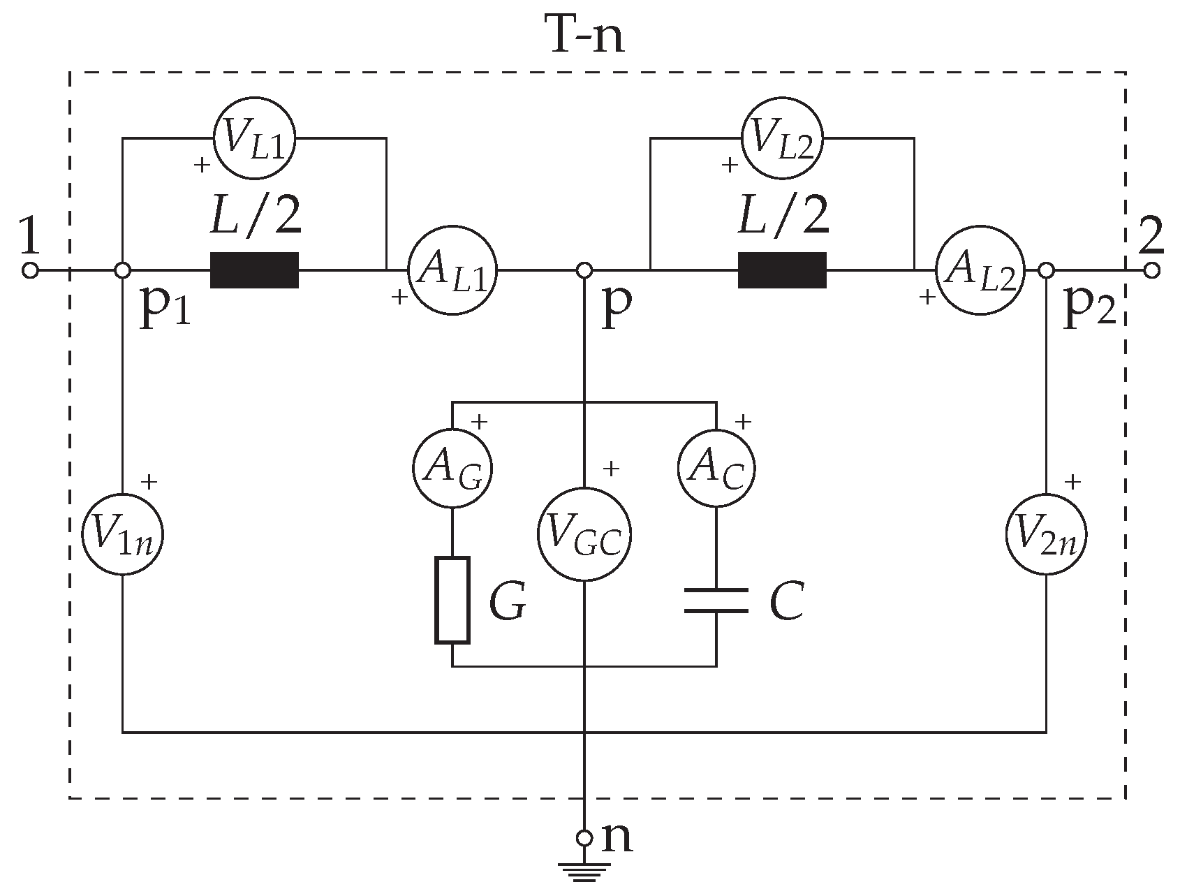
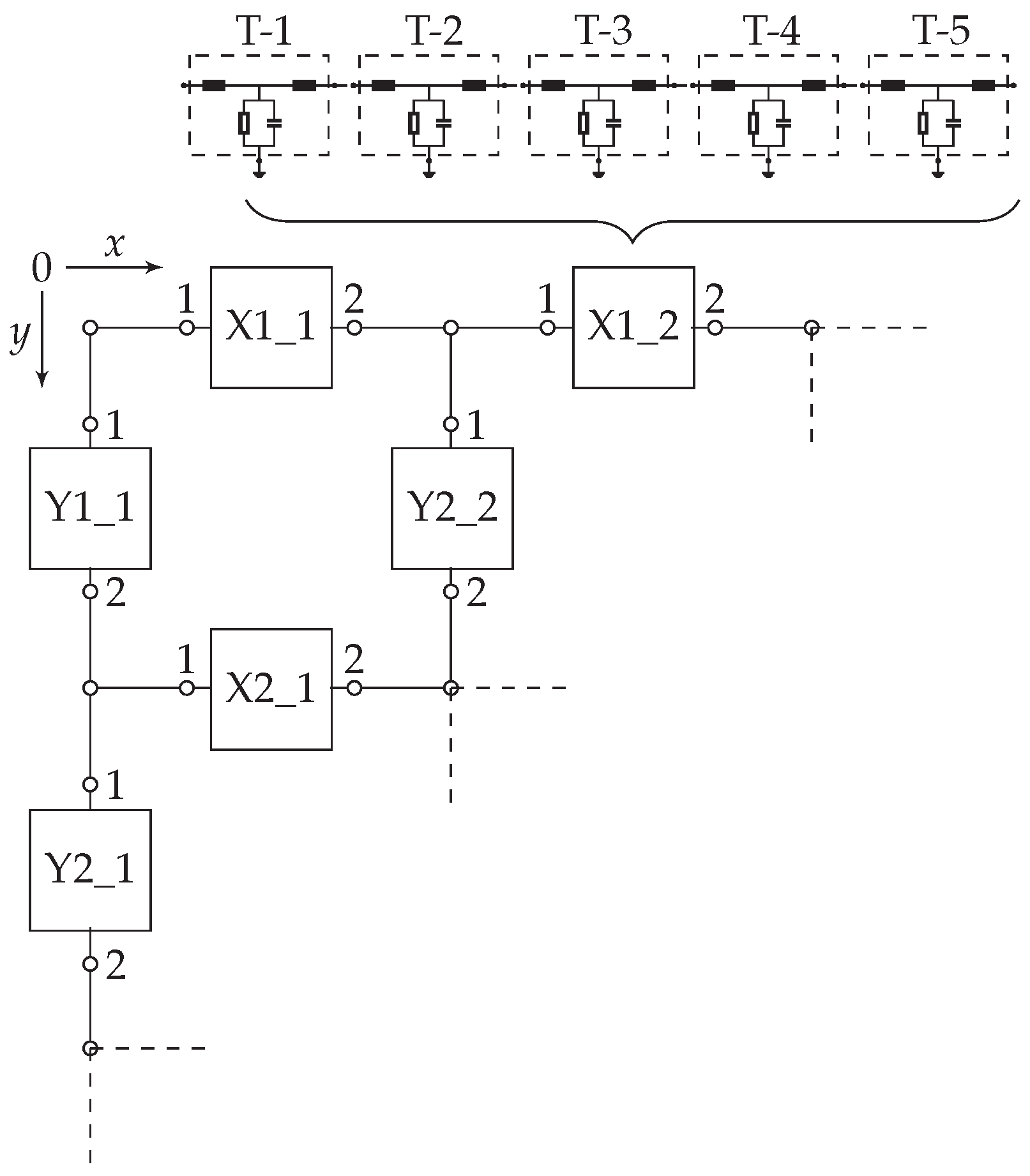
The element length in per-unit model of the grounding wire is implemented in Matlab as a T-section of the transmission line model. The grounding wire implementation is illustrated with fundamental electrical elements and measurement nodes in Figure 1 which forms a horizontal buried grounding wire. From the grounding wire t-section development, the grounding system is implemented by an appropriate number of T-sections and additional nodes using Simulink graphical block elements. The grounding system layout with formation strategy is illustrated Figure 2 which gives references to the simulation database is found in Appendix B. To assure a smooth representation of the interconnection between elements, and to possibly extend the model functionality to include mutual couplings, the T-section represent one meter of ground wire (in per-unit) [4]. Consequently, the model can be extended to arbitrary lengths and configurations.
This consideration gives the total number of required logged variables for the formed horizontal buried grounding grid square meshes as an indication for two different mesh sizes and total area in Table 1.
As described trough Section 2 the grounding system is modelled as a transmission line, connecting the soil and grounding conductor properties. The matrices of the grounding system may be expressed trough the coupled telegraphers equations in frequency domain trough Equation (6). Where and are the line phasor of voltage and current [10]:
In transient analysis, considering the spatial distribution of voltage potential and current flowing in the grounding system, it is mandatory to simulate each element in time domain. With the layout of grounding grids, as is illustrated Equation (2), several connection points exists. Consequently, the time domain model is required to account for the coupling between elements as feeding points. For J feeding points the impact of the grounding system, as an electrical network exited by an injected lightning current, is global. Each element in the grounding system matrices is numerically solved independently by the Matlab ODE23t solver, which implements the trapezoidal rule using a “free” interpolation for the time domain solution. The implementation account for the injected current characteristics and corresponding frequency response of the grounding system.
4. Grounding Model Verification
The grounding system model is validated by the work based on the ElectroMagnetic Field (EMF) theory first performed by Grcev [11] and later by Jardines et al. [7] who introduced a variant of the Multi-conductor Transmission Line (MTL) approach. In these cases of model verifications, the current source is implemented using the double exponential waveform, , and the source parameters where adjusted to fit the given stroke function. The referenced work is reproduced from manual reading.
4.1. Grounding Rod of 15 m Length
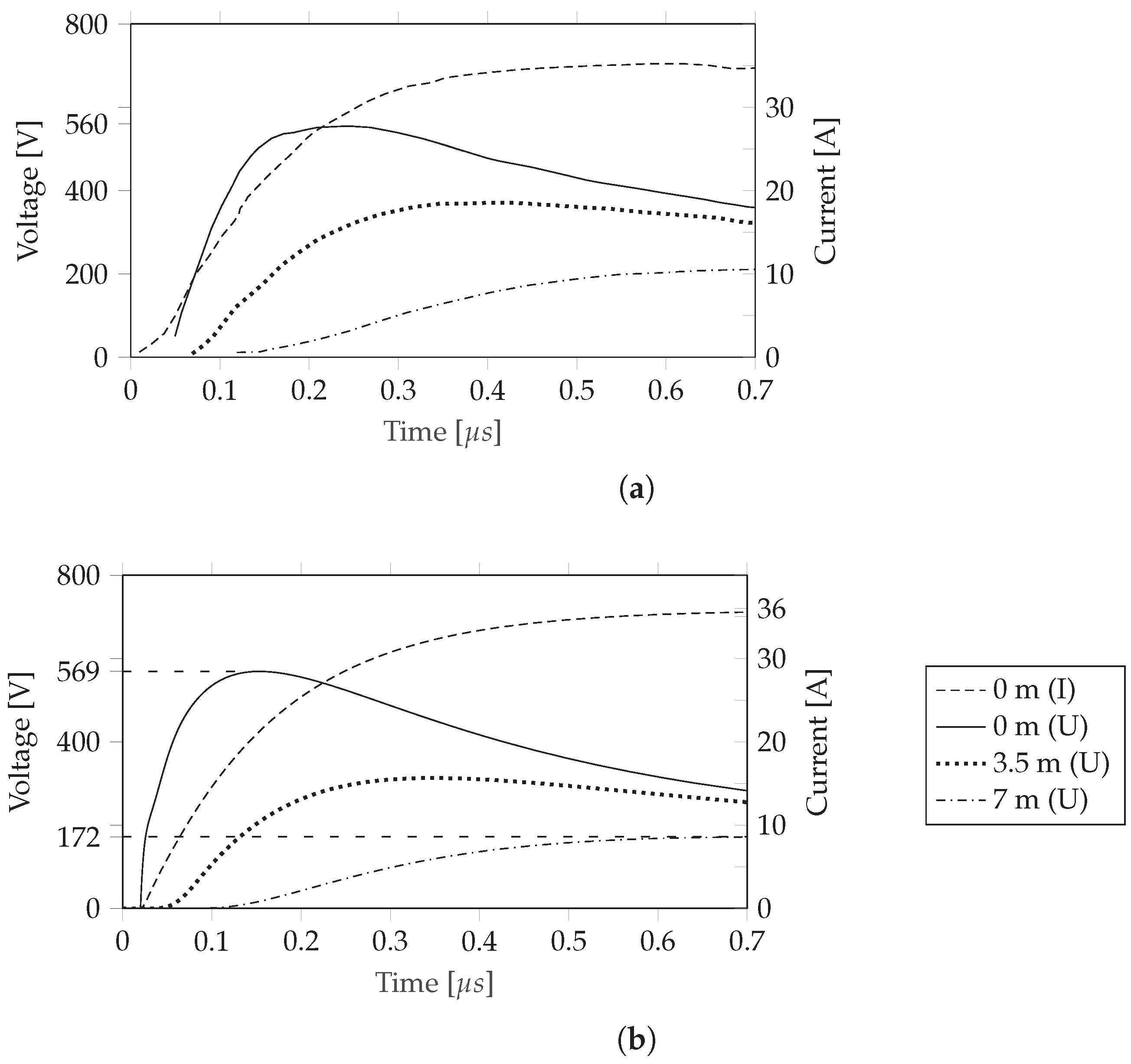
A grounding rod of 15 m was simulated and measured by Grcev [11] and later evaluated by Jardines et al. [7] as shown in Figure 3a. Using two independent modeling approaches and relative similarities in results may justify the present modeling accuracy. The grounding rod is horizontally buried in soil of = 70 m and = 15, with a wire radius of a = 0.012 m at depth d = 0.6 m. The current source was set with the amplitude of = 36 A and the stroke of 0.36/12 s which leads to the new parameter values = 32 × 10 and = 7.6 × 10. The results from the implemented model are shown in Figure 3b. As it can be observed from Figure 3a in the referenced work, the peak values at the injection point are approximately 560 V. While using the implemented model, Figure 3b, the peak value shows 569 V. The second point for comparison is at 7 m from the injection point where Grcev simulations show approximate 200 V while the results in this work gives 172 V after 0.7 s. Besides the point value readings, the surge wave propagation along the grounding rod and voltage distribution are of similar character.
4.2. Grounding Grid of 10 m Meshes with Total Size 3600 m
A grounding system of 10 × 10 m meshes size and a total square area of 3600 m was simulated by Jardines et al. [7] using a variant of the MTL approach (see Figure 4a). The grounding grid was buried in soil of = 100 m and = 36, with a wire radius of American Wire Gauge (AWG) 2/0 (a ≈ 0.004126 m) at depth d = 0.6 m. The current source was set with amplitude of = 1 kA and a 1/20 s which gave adjusted parameters to = 38 × 10 and = 2.54 × 10. The results from the implemented model are given in Figure 4b. Since the injected current was not given in the referenced work (see Figure 4a) it is worth noting that a small deviation in the injected current will have a large impact on the grounding system response, especially for the region contributing to limiting the peak voltage. As it can be observed, both the voltage distribution and the propagation characteristics correspond well. When comparing the simulation to Grcev [11] which was based on EMF against the simulation in the presented work, the peak value and the propagation characteristics are of comparable values. However, the distributed voltage at the given nodal points is more conservative in the transmission line approach, both in the implemented model and in Jardines et al. work [7]. This unveils a model accuracy difference compared to the EMF. As reviewed, Liu [4] developed the non-uniform transmission line approach to compensate for the inaccuracy of this method and are treated in details in her work.
5. Integration of Grounding and Transmission System
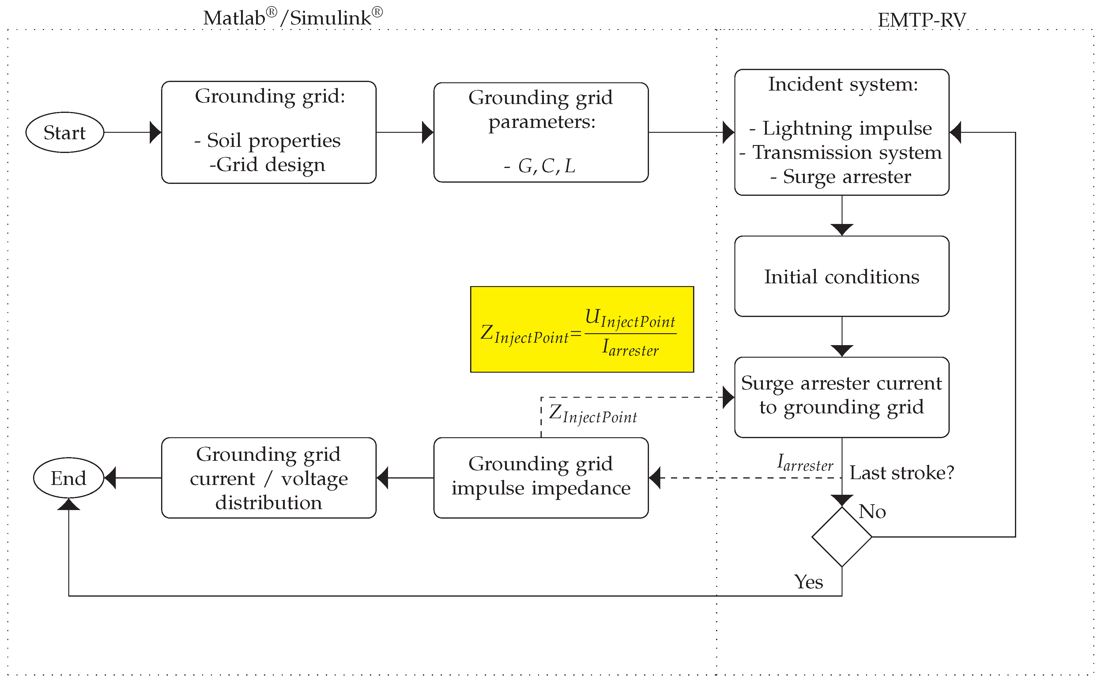
The Matlab/Simulink grounding grid are integrated with EMTP-RV through a newly developed FMI software, which was released by Powersys Solutions in early 2018 [12,13]. The FMI package gives possibilities for co-simulation with information exchange at a per simulation time-step interval (sequentially processed). The specific FMI interface used in this study is found in Appendix A.2. From the transmission system surge arrester, the injection point impedance describes the grounding system response trough Equation (7).
When the transmission system surge arrester reaches the breakdown voltage a current surge is injected into the grounding system. The current injection value is exchanged from EMTP-RV to Matlab, which simulates the grounding system response. The grounding system initial impedance is set to the power frequency value corresponding to the grounding system resistance [14]. From the injection point current and the induced voltage potential rise, the impulse impedance is calculated and exchanged from Matlab to EMTP-RV, which connects the dynamic response of the grounding system to the transmission system. With a large number of logged variables required by the grounding system (see Table 1) and presented implementation strategy, the additional measured values of the transmission system were exchanged from EMTP-RV to Matlab to provide a common simulation log for pre-processing. The advanced functionality offered by the Matlab/Simulink modeling of the grounding system lies in the preprocessing of large data-sets. A schematic overview of the model integration is illustrated in Figure 5.
6. An Example of Results: Case Study
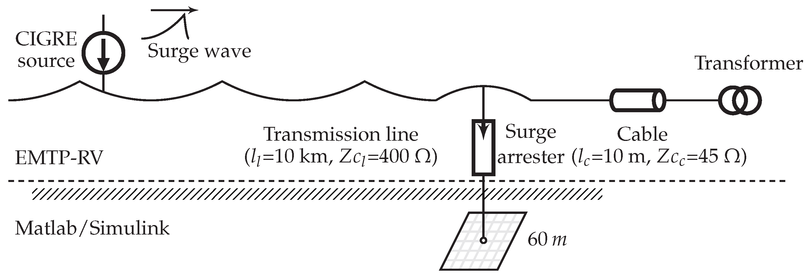
A simplified transmission system network is shown in Figure 6 with the grounding system model interfaced in Matlab. In this model the transmission line, the cable, the transformer and the surge arrester are selected from the standard EMTP-RV software library. At 10 km distance from a substation, a lightning strikes the 300 kV overhead transmission line ( = 400 ). A shielding failure causes an injected current with a magnitude of 1 kA and 1.2/50 s of CIGRE waveform stroke to flow towards the substation. In the substation, the cable () between the surge arrester (Appendix C) and transformer are 10 m. Figure 7 shows the simulation results of the transmission system when the grounding system is ignored, thus giving a peak voltage of 171 kV at the transformer.
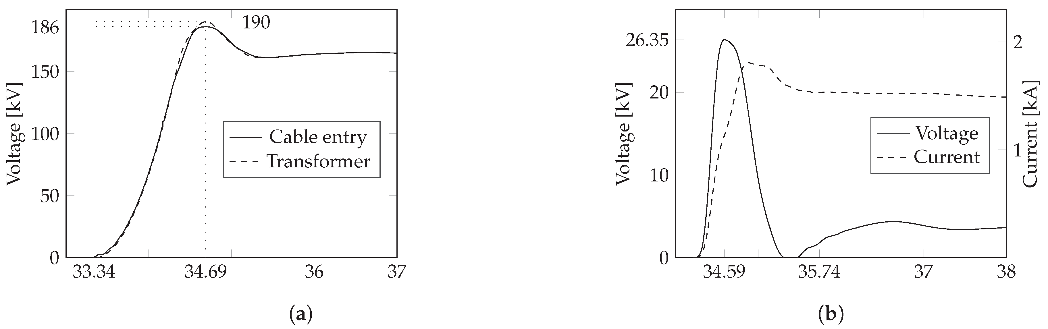
A grounding system with 10 × 10 m mesh size is added with a total grid area of 3600 m in soil of = 2000 m, = 16, with a wire radius of a = 0.04126 m at depth d = 0.6 m is obtained. The transmission system conditions are similar. The surge arrester is connected in center of the grid. The simulation results of the transmission system are given in Figure 8. As it can be observed, the surge arrester performance is reduced to give a peak transformer voltage of 190 kV.
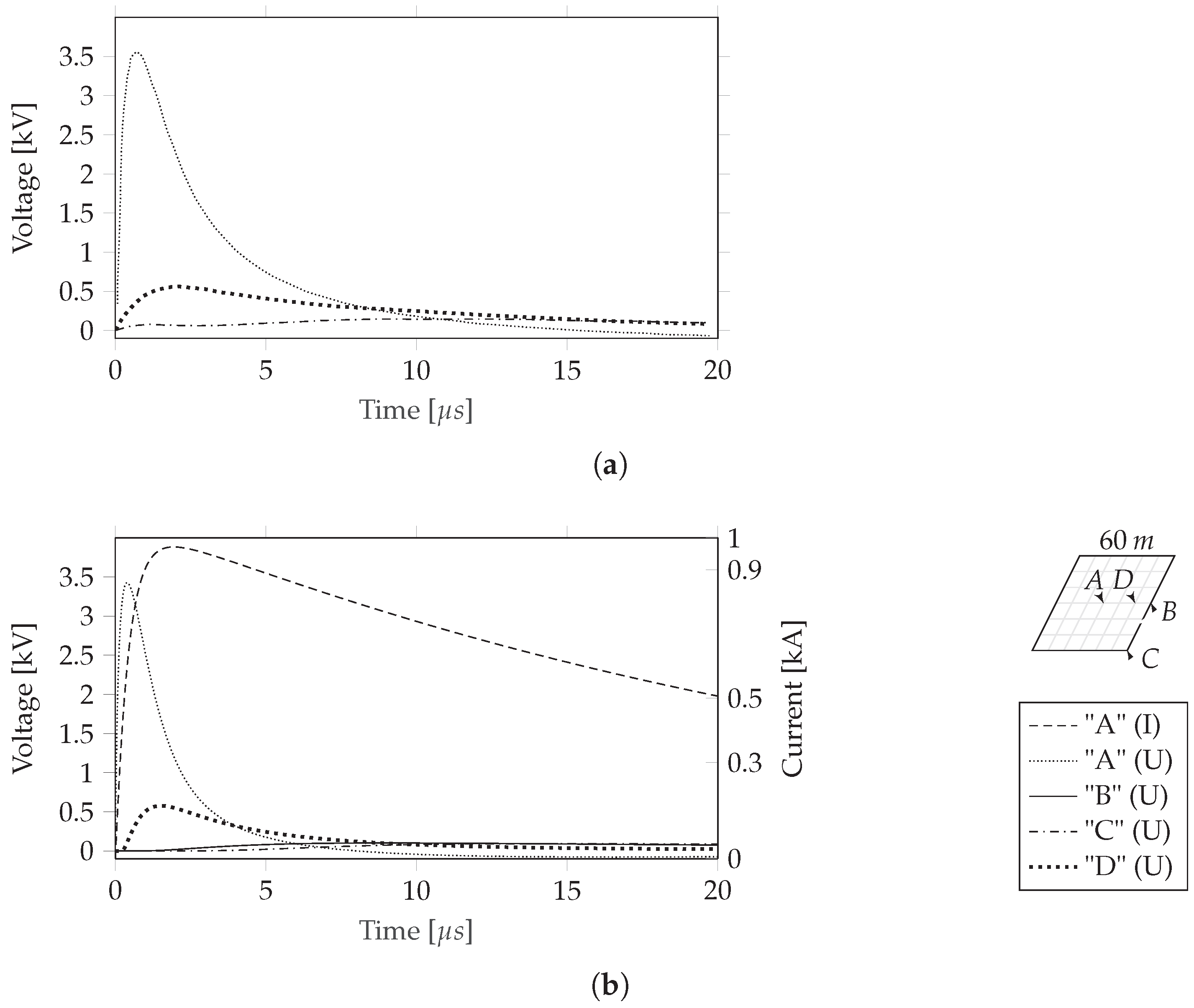
Then, the EMI analysis of the substation could be performed based on the overall voltage distributions in the grounding system as shown in Figure 9. Figure 9a shows measurments of the grounding system, with nodal points selected diagonaly outwards from the center injection point. For the selected events an overall voltage distribution is presented. Figure 9b shows the distribution at center peak voltage and Figure 9c when the voltage potential in the grid corners are at peak.
With the comprehensive log dataset further analysis is exemplified in Figure 10 and Figure 11. The impulse effective area of the grounding grid defined in [15] is shown in Figure 10. This is the total area of the grounding grid which limits the peak voltage in the grid. There exists several definitions and empirical formulas for estimating the effective length when optimizing the grounding grid design that was recently evaluated [5]. However, these approaches have not taken the transmission line network itself as an integrated element into consideration. In addition, the electric field exerted on the soil close to the grounding wires that was based on the current density leaked to the soil is shown in Figure 11.
Institute of Electrical and Electronics Engineers (IEEE) indicates (quoted in standard) a critical breakdown value of = 1000 kV/m [16] (p. 1263). This definition gives reference to the above mentioned experimental relation between soil resistivity and [17]. Further evaluation of IEEE standards gives a value of = 400 kV/m, a level which are referred without reference in [18] (p. 38) (refereed standard is currently under review for update). If the ionization level is reached the electric field in the soil has pronounced influence on the impulse peak voltage. Moreover, ionization has a positive effect by lowering the peak voltage due to arcing or puncturing in the soil. Soil ionization can be included in dynamic simulations as it has been proposed in [9]. This would modify the apparent grounding conductor radius in Equations (2) and (3). For this application case when considering strokes in the transmission system, soil ionization phenomena has been evaluated to have minor deviation of the results due to relative small currents injected trough the surge arrester.
7. Conclusions
The new modeling approach allows integration of the grounding system into the transmission system when analyzing the lightning surge performance of the transmission system. By using the more detailed Matlab/Simulink model presented in this work, large data-sets are processed to extract overall measured values in EMI analysis. Different functions and parameters may be processed by the simulation log of the grounding system and parameters such as the effective length and the electric field distribution. Moreover, by taking advantage of the newly developed FMI interface, the grounding grid model itself is integrated as an element in the transmission system modeling and analysis by EMTP-RV. Lastly, the surge arrester performance is better assessed when the grounding system is included and consequently, the corresponding effects of all parts in the transmission system could be more accurately analyzed.
The grounding system model presented in this work is simplified and neglect significant factors of a physical system. Moreover, with the implementation of the grounding system in Matlab/Simulink features flexibility and significant potential for further development so that the accuracy could be improved.
Author Contributions
V.S. developed the method, performed simulation/data analysis and prepared the manuscript as the first author. L.H.S., S.Z. and E.C. assisted the project with insights in the method development phase and review process. All authors discussed the results and approved the publication.
Funding
This research received no external funding
Acknowledgments
The authors thank for the support given by Western Norway University of Applied Sciences and the University of Bergen to carry out this work. A special thank to International Conference on High Voltage Engineering and Application (ICHVE) 2018 for the invitation to publish in this special issue entitled “Selected Papers from 2018 IEEE International Conference on High Voltage Engineering”.
Conflicts of Interest
The authors declare no conflict of interest.
Glossaries
| Symbol | Unit | Description | Page(s) |
| a | m | Grounding conductor radius...................................... | 2, 4, 5, 7 |
| - | Decay constant of double exponential source...................... | 4–6 | |
| - | Crest constant of double exponential source....................... | 4–6 | |
| C | F | General term describing capacitance............................. | 2 |
| d | m | Grounding conductor burial depth................................ | 2, 4–7 |
| V/m | Critical electric field for soil ionization............................ | 2, 8 | |
| V/m | Electric field strenght exerted on the soil.......................... | 2 | |
| G | S | General term describing conductance............................. | 2 |
| I | A | General term describing current................................... | 6 |
| A | Current leaked from the ground per-unit lenght conductor to the soil................................................................ | 2 | |
| A | Current magnitude of double exponential source.................. | 4–6 | |
| A/m | Current density leaked to the soil................................. | 2 | |
| L | H | General term describing inductance............................... | 2 |
| s | m | Grounding conductor spacing. | |
| l | m | General term describing length................................... | 2, 5, 8 |
| - | MOA Exponential factor to form the V-I characteristic............. | 12, 13 | |
| - | MOA Voltage segment factor to form the V-I characteristic........ | 12, 13 | |
| V | MOA Reference voltage for operation............................. | 12, 13 | |
| H/m | Permeability of vacuum: 4π × 10−7. | 2 | |
| - | Relative permittivity of the soil.................................... | 2, 4–7 | |
| F/m | Permittivity of vacuum: ......................... | 2 | |
| m | Resistivity of soil.................................................. | 2, 4–7 | |
| U | V | General term describing voltage.................................. | 6 |
| Y | S | General term describing admittance............................... | 2, 4 |
| Z | General term describing impedance............................... | 2, 4 | |
| - | Cable surge impedance based on the lossless transmission line model ............................................................ | 7 | |
| - | Transmission line surge impedance based on the lossless transmission line model........................................... | 7 |
Abbreviations
| Symbol | Description | Page(s) |
| AWG | American Wire Gauge ............................................ | 5, 6 |
| CIGRE | Conseil International des Grands Réseaux Électriques............. | 1 |
| EMF | ElectroMagnetic Field. | 4, 5 |
| EMI | ElectroMagnetic Interference ...................................... | 1, 2, 8 |
| ICHVE | International Conference on High Voltage Engineering and Application ....................................................... | 10 |
| IEEE | Institute of Electrical and Electronics Engineers ................... | 8 |
| MTL | Multi-conductor Transmission Line ............................... | 4, 5 |
Appendix A. Software and Integration
Appendix A.1. Software Versions
All simulations were performed on a standard consumer laptop computer with Intel Core I7-2640M (dual-core, 2.70GHz, 4MB Cache) CPU and 8 GB (1333 MHz) RAM. The Matlab/Simulink grounding grid models was developed and tested on 64-bit Microsoft Windows 10 Pro version 1709.
Windows version:
- MathWorks Matlab version 9.3, R2017b, 64-bit (14 September 2017)
- MathWorks Simulink version 9.0, R2017b, 64-bit (24 July 2017)
- MathWorks Simscape version 4.3 (18 November 2017)
Powersys EMTP-RV
- Powersys EMTP-RV 3.5 32-bit (17 January 2017)
- Powersys FMI Add-On for Matlab/Simulink (15 March 2018)
Appendix A.2. Matlab/Simulink and EMTP-RV FMI Interface
Figure A1.
The Matlab/Simulink FMI interface to EMTP-RV with the signals transferred between the softwares and block representation of the integration.
Figure A1.
The Matlab/Simulink FMI interface to EMTP-RV with the signals transferred between the softwares and block representation of the integration.

Appendix B. Matlab/Simulink Simulation Log Definition
Values from the implemented measurement nodes, for each grounding wire t-section as illustrated by Section 3 and Figure 1, are stored in a simulation-log database. The simulation-log database is organized with value identifications from the t-section measurements definitions in addition to the grounding grid formation strategy, Figure 2, and forms nodal points connection to physcial properties.

Table A1.
Simulation-log nodal measurement overview and grounding system variable definitions.
| Node (Figure 1) | Log-File Name | Grid Segment (Figure 2) | Element | Series Selection |
|---|---|---|---|---|
| simlog_scc_grounding_system. | X/Y’y-dir’_’x-dir’. | l1.v. | series.values/time | |
| simlog_scc_grounding_system. | X/Y’y-dir’_’x-dir’. | l1.i. | series.values/time | |
| simlog_scc_grounding_system. | X/Y’y-dir’_’x-dir’. | l2.v. | series.values/time | |
| simlog_scc_grounding_system. | X/Y’y-dir’_’x-dir’. | l2.i. | series.values/time | |
| simlog_scc_grounding_system. | X/Y’y-dir’_’x-dir’. | p1.v. | series.values/time | |
| simlog_scc_grounding_system. | X/Y’y-dir’_’x-dir’. | p2.v. | series.values/time | |
| simlog_scc_grounding_system. | X/Y’y-dir’_’x-dir’. | g.i. | series.values/time | |
| simlog_scc_grounding_system. | X/Y’y-dir’_’x-dir’. | p.v. | series.values/time | |
| simlog_scc_grounding_system. | X/Y’y-dir’_’x-dir’. | c.i. | series.values/time |
Appendix C. EMTP-RV Surge Arrester Parameterization V-I characteristics
Surge arrester switching and damping interaction is according to standard by EMTP-RV model number: 865630. The surge arrester is parameterized according to the overview below. Where is a fitting constant (-), is a coefficient of non-linearity (-) and (pu) is a factor of the arrester system voltage (-).
| Segment | (pu) | ||
|---|---|---|---|
| 1 | 4.23208099271728 × 10 | 2.40279296219991 × 10 | 2.98198270953446 × 10 |
| 2 | 2.81773645053899 × 10 | 2.66219333383972 × 10 | 4.81500000000002 × 10 |
| 3 | 4.15144087019289 × 10 | 2.00870413085783 × 10 | 5.24450368910346 × 10 |
| 4 | 2.63271405014350 × 10 | 3.52906710089596 × 10 | 5.62230840318764 × 10 |
| 5 | 3.21774149817822 × 10 | 1.11310570543270 × 10 | 5.69192036592734 × 10 |
| 6 | 1.93774621300766 × 10 | 5.36270125014300 | 6.14408449804349 × 10 |
References
- IEEE. 80-2013—IEEE Guide for Safety in AC Substation Grounding; IEEE Std 80-2013 (Revision of IEEE Std 80-2000/Incorporates IEEE Std 80-2013/Cor 1-2015); IEEE: New York, NY, USA, 2015; pp. 1–226. [Google Scholar] [CrossRef]
- Sunde, E.D. Earth Conduction Effects in Transmission Systems, 1st ed.; The Bell Telephone Laboratories, Dover Publications: New York, NY, USA, 1949. [Google Scholar]
- Grcev, L.; Dawalibi, F. An Electromagnetic Model for Transients in Grounding Systems. IEEE Trans. Power Deliv. 1990, 5, 1773–1781. [Google Scholar] [CrossRef]
- Liu, Y. Transient Response of Grounding Systems Caused by Lightning: Modelling and Experiments. Ph.D. Thesis, Uppsala University, Uppsala, Sweden, 2004. [Google Scholar]
- Grcev, L. Lightning Surge Efficiency of Grounding Grids. IEEE Trans. Power Deliv. 2011, 26, 1692–1699. [Google Scholar] [CrossRef]
- Alipio, R.; Schroeder, M.A.O.; Afonso, M.M. Voltage Distribution Along Earth Grounding Grids Subjected to Lightning Currents. IEEE Trans. Ind. Appl. 2015, 51, 4912–4916. [Google Scholar] [CrossRef]
- Jardines, A.; Guardado, J.L.; Torres, J.; Chávez, J.J.; Hernández, M. A Multiconductor Transmission Line Model for Grounding Grids. Int. J. Electr. Power Energy Syst. 2014, 60, 24–33. [Google Scholar] [CrossRef]
- Liu, Y.; Theethayi, N.; Thottappillil, R. An Engineering Model for Transient Analysis of Grounding System under Lightning Strikes: Nonuniform Transmission-Line Approach. IEEE Trans. Power Deliv. 2005, 20, 722–730. [Google Scholar] [CrossRef]
- He, J.; Gao, Y.; Zeng, R.; Zou, J.; Liang, X.; Zhang, B.; Lee, J.; Chang, S. Effective Length of Counterpoise Wire under Lightning Current. IEEE Trans. Power Deliv. 2005, 20, 1585–1591. [Google Scholar] [CrossRef]
- Alipio, R.; Costa, R.M.; Dias, R.N.; Conti, A.D.; Visacro, S. Grounding Modeling Using Transmission Line Theory: Extension to Arrangements Composed of Multiple Electrodes. In Proceedings of the 2016 33rd International Conference on Lightning Protection (ICLP), Estoril, Portugal, 25–30 September 2016; pp. 1–5. [Google Scholar] [CrossRef]
- Grcev, L.D. Computer Analysis of Transient Voltages in Large Grounding Systems. IEEE Trans. Power Deliv. 1996, 11, 815–823. [Google Scholar] [CrossRef]
- Modelica Association c/o PELAB. Functional Mock-Up Interface. 2018. Available online: http://fmi-standard.org/ (accessed on 23 March 2018).
- Cornau, J. Guide EMTP-RV Matlab/Simulink FMI Export; Powersys: Paris, France, 2018. [Google Scholar]
- IEEE. IEEE Guide for Measuring Earth Resistivity, Ground Impedance, and Earth Surface Potentials of a Grounding System; IEEE Std 81-2012 (Revision of IEEE Std 81-1983); IEEE: New York, NY, USA, 2012; pp. 1–86. [Google Scholar] [CrossRef]
- Gupta, B.R.; Thapar, B. Impulse Impedance of Grounding Grids. IEEE Trans. Power Appar. Syst. 1980, PAS-99, 2357–2362. [Google Scholar] [CrossRef]
- Estimating Lightning Performance of Transmission Lines. II. Updates to Analytical Models. IEEE Trans. Power Deliv. 1993, 8, 1254–1267. [CrossRef]
- Oettle, E.E. A New General Estimation Curve for Predicting the Impulse Impedance of Concentrated Earth Electrodes. IEEE Trans. Power Deliv. 1988, 3, 2020–2029. [Google Scholar] [CrossRef]
- IEEE. IEEE Guide for the Application of Insulation Coordination; IEEE Std 1313.2-1999; IEEE: New York, NY, USA, 1999. [Google Scholar] [CrossRef]
- Hagen, S.T. Lightning Strike Analysis; Western Norway University of Applied Sciences: Porsgrunn, Norway, 2016. [Google Scholar]
Figure 1.
Element lenght in per-unit grounding wire illustration of implementation.

Figure 2.
The grounding system layout with formation strategy.

Figure 3.
Voltage distribution along an horizontal copper wire in ground (length l = 15 m, conductor radius a = 0.012 m, at soil depth d = 0.6 m) in soil of = 70 m and = 15: (a) the reproduced results for comparison from the research given in [11] (p. 818); and (b) results from implemented model with excitation current = 36 A of double exponential waveform ( = 32 × 10, = 7.6 × 10).

Figure 4.
Voltage distribution in a grounding grid consisting of 6 × 6 meshes of 10 m size. The grounding grid consist of copper conductors of AWG 2/0, buried at d = 0.6 m in soil of = 100 m and = 36: (a) the reproduced results for comparison from research given in [7] (p. 31); and (b) results from implemented model with excitation current = 1 kA of double exponential waveform ( = 38 × 10, = 2.54 × 10).

Figure 5.
Schematic overview of the integration between grounding and transmission system.

Figure 6.
Simplified illustration of implemented transmission and grounding system.

Figure 7.
Ignoring grounding system: transmission system nodal voltages and CIGRE 1.2/50 s injected current stroke in far-end (l = 10 km).
Figure 7.
Ignoring grounding system: transmission system nodal voltages and CIGRE 1.2/50 s injected current stroke in far-end (l = 10 km).

Figure 8.
Application case when the grounding system is added: (a) the effect in the transmission system; and (b) the results at the surge arrester injection point.
Figure 8.
Application case when the grounding system is added: (a) the effect in the transmission system; and (b) the results at the surge arrester injection point.

Figure 9.
Application case when the grounding system is added: (a) nodal voltage measurement values for selected points in the grounding grid; (b) the overall voltage distribution in the grounding grid at peak; and (c) the overall voltage distribution in the grounding grid at corner peak.
Figure 9.
Application case when the grounding system is added: (a) nodal voltage measurement values for selected points in the grounding grid; (b) the overall voltage distribution in the grounding grid at peak; and (c) the overall voltage distribution in the grounding grid at corner peak.

Figure 10.
Application case: used area.

Figure 11.
Application case: peak field.

Table 1.
Required number of logged variables for grounding grid of two different square mesh sizes and total area values.
Table 1.
Required number of logged variables for grounding grid of two different square mesh sizes and total area values.
| Grounding Grid | Area | Variables |
|---|---|---|
| 5 × 5 m mesh | 1600 m | 6480 |
| 3600 m | 14040 | |
| 10 × 10 m mesh | 1600 m | 3600 |
| 3600 m | 7560 |
© 2019 by the authors. Licensee MDPI, Basel, Switzerland. This article is an open access article distributed under the terms and conditions of the Creative Commons Attribution (CC BY) license (http://creativecommons.org/licenses/by/4.0/).
Share and Cite
MDPI and ACS Style
Steinsland, V.; Sivertsen, L.H.; Cimpan, E.; Zhang, S. A New Approach to Include Complex Grounding System in Lightning Transient Studies and EMI Evaluations. Energies 2019, 12, 3142. https://doi.org/10.3390/en12163142
AMA Style
Steinsland V, Sivertsen LH, Cimpan E, Zhang S. A New Approach to Include Complex Grounding System in Lightning Transient Studies and EMI Evaluations. Energies. 2019; 12(16):3142. https://doi.org/10.3390/en12163142
Chicago/Turabian StyleSteinsland, Vegard, Lasse Hugo Sivertsen, Emil Cimpan, and Shujun Zhang. 2019. "A New Approach to Include Complex Grounding System in Lightning Transient Studies and EMI Evaluations" Energies 12, no. 16: 3142. https://doi.org/10.3390/en12163142
Note that from the first issue of 2016, this journal uses article numbers instead of page numbers. See further details here.