Article

Maximum Power Point Tracker Based on Fuzzy Adaptive Radial Basis Function Neural Network for PV-System

by
Noureddine Bouarroudj
1,
Djamel Boukhetala
2,
Vicente Feliu-Batlle
3,*,
Fares Boudjema
2,
Boualam Benlahbib
1 and
Bachir Batoun
1
1
Unité de Recherche Appliquée en Energies Renouvelables, URAER, Centre de Développement des Energies Renouvelables, CDER, Ghardaïa 47133, Algeria
2
Laboratoire de Commande des Processus, Ecole Nationale Polytechnique, 10 Rue des Frères OUDEK, El-Harrach, Alger 16200, Algeria
3
School of Industrial Engineering, University of Castilla-La Mancha, Av. Camilo Jose Cela, S/N, C.P. 13001 Ciudad Real, Spain
*
Author to whom correspondence should be addressed.
Energies 2019, 12(14), 2827; https://doi.org/10.3390/en12142827
Submission received: 14 June 2019 / Revised: 15 July 2019 / Accepted: 16 July 2019 / Published: 22 July 2019
(This article belongs to the Section A2: Solar Energy and Photovoltaic Systems)

Abstract

:
In this article, a novel maximum power point tracking (MPPT) controller for a photovoltaic (PV) system is presented. The proposed MPPT controller was designed in order to extract the maximum of power from the PV-module and reduce the oscillations once the maximum power point (MPP) had been achieved. To reach this goal, a combination of fuzzy logic and an adaptive radial basis function neural network (RBF-NN) was used to drive a DC-DC Boost converter which was used to link the PV-module and a resistive load. First, a fuzzy logic system, whose single input was based on the incremental conductance (INC) method, was used for a variable voltage step size searching while reducing the oscillations around the MPP. Second, an RBF-NN controller was developed to keep the PV-module voltage at the optimal voltage generated from the first stage. To ensure a real MPPT in all cases (change of weather conditions and load variation) an adaptive law based on backpropagation algorithm with the gradient descent method was used to tune the weights of RBF-NN in order to minimize a mean-squared-error (MSE) criterion. Finally, through the simulation results, our proposed MPPT method outperforms the classical P and O and INC-adaptive RBF-NN in terms of efficiency.

Graphical Abstract

1. Introduction

Nowadays, one of the most important alternative energy sources is solar energy. Several efforts and research have been concentrated on improving the efficiency of PV systems and the accessibility of this technology.
Photovoltaic systems are built using one or more photovoltaic modules, a DC load, and a DC-DC power converter which links the PV-module and the load. The PV-module has an MPP at a specific load value. This point is not stable; it undergoes variations in accordance with some parameters that modify the functionality of the PV-system, like the solar irradiation and the temperature. This makes it necessary to use a control technique capable of acting on the duty cycle of the DC-DC converter in order to be able to track the MPP of the PV system.
Several algorithms have been reported in the literature for MPP searching, such as the Hill Climbing method [1,2], the Incremental Conductance (INC) method [3], the Perturb and Observe (P and O) algorithm [4,5,6], the fractional open circuit [7] and the short-current algorithm [8]. These MPPT techniques present different complexities, hardware implementations and convergence speeds.
While the maximum power delivered by the PV-module changes with atmospheric conditions like temperature and irradiance, and because the PV-module exhibits non-linear ppv-vpv and ipv-vpv characteristics, most of these MPPT techniques lack a perfect convergence to the MPP, and usually present oscillations around the MPP [9] due to the voltage fixed-step-size (Δv) used to perturb (or update) the PV-module voltage. To overcome these problems, some works have been reported in the literature, such as References [10,11,12,13], based on a variable step size. The step size is automatically tuned according to the PV-module characteristics (ppv-vpv curve). In Reference [14], a second stage is added to the classical P and O algorithm in order to reduce the steady-state oscillation and correct the asymmetric operating point of the PV-module.
Nowadays, MPPT controllers based on artificial intelligence have gained interest because of the theoretical and practical studies reported in the literature. MPPT controls based on fuzzy logic, including the two alternatives of Mamdani and Takagi-Sugeno, are examples of this. They allow many approaches and schemes depending on the number (and nature) of inputs, outputs and linguistic variables. The authors in References [15,16] have proposed a fuzzy MPPT controller that uses two inputs, the error (E) and the change of error (CE), and one output which is the change of duty cycle. Error E = ∂ppv/∂vpv was chosen in Reference [15] while an error E = ∂ppv/∂ipv was chosen in Reference [16]. A fuzzy MPPT controller with a single input was studied in Reference [17]. In order to obtain optimal results, evolutionary algorithms have been used for tuning the parameters of these controllers, like in References [18,19,20]. A fuzzy logic MPPT controller with adaptive gain has also been proposed in Reference [21]. For the oscillation reduction (to practically zero) in the steady-state once the MPP has been reached, MPPT controllers that only use evolutionary computation techniques have been proposed, such as particle swarm optimization in References [22,23,24], artificial fish-swarm algorithm in Reference [25], and the cuckoo search algorithm in Reference [26].
On the other hand, in order to tackle the disadvantages of the classical methods, several approaches for MPPT based on artificial neural networks (ANN) have been considered. The first class of the ANN approaches uses the ambient climatic conditions (irradiation and temperature) to estimate the optimum voltage/current, or both the voltage and the current [27,28,29,30,31,32], or uses the climatic conditions to estimate the duty cycle [33,34], in order to ensure the maximum power point operation. A second approach uses the PV-module current and voltage to estimate the optimum voltage [35,36,37], or duty cycle [38,39,40]. In order to obtain high precision and fast convergence, some researchers have combined fuzzy logic with ANN to design alternative schemes called, respectively, the ANFIS-based MPPT controller [41], the neuro-fuzzy MPPT controller [42] and the neural network optimized fuzzy logic controller for MPPT [43].
Most of the approaches proposed to estimate the optimum voltage, or voltage and current, are implemented in the second stage of the control system classical PI or PID controllers that deliver the duty cycle used to control the DC-DC converter. These controllers are easy to design and simple to implement. However, they have some drawbacks such as the dependence of the performance on the working point, the necessity of returning the controller parameters when changes in the reference voltage or load parameters are produced, and the complexity of designing the controller parameters and the associated stabilization problems, etc. To overcome these limitations, the use of fuzzy logic controllers (FLC) was proposed in Reference [44] because of its advantages: it is nonlinear, robust and adaptive in nature. The FLC inputs are usually the voltage error and the change of error.
Motivated by the above discussion, this paper proposes a novel fuzzy-adaptive RBF neural network MPPT controller for a PV system, which is built with a PV-module, a DC-DC boost converter and a resistive load. The MPPT controller contains two stages. In the first one, we have used a fuzzy controller with a single input to generate a variable voltage step size (Δv) based on the incremental conductance algorithm concept. The input of the FLC is the sum of instantaneous conductance and its incremental ( E = i pv v pv + i pv v pv ). Its output is the voltage step size (Δv), in which the range of both variables E and Δv is decomposed into five linguistic variables (negative big, negative small, zero, positive small, positive big). By this way, the output Δv can be regulated according to the distance between the operating point of the PV-module and the MPP, which can suppress the oscillations when the MPP is reached. In the second stage, and in order to tackle the problems of conventional PID controllers, we have used an RBF-NN with a voltage error (e = vpv-vopt) at its input, to calculate the duty cycle (α) in order to keep vpv at vopt. The weights of the RBF-NN have been on-line adjusted by using a backpropagation algorithm combined with the gradient-descent method in order to minimize an MSE criterion. The simulation results using the Matlab/Simulink program under four scenarios: standard climatic condition (T = 25 °C, S = 1000 W/m2), slope variation of the irradiance, resistive-load step changes, and real daily profile of irradiance and temperature, show the superiority of the proposed MPPT algorithm over the standard P and O algorithm and the INC-adaptive RBF neural network algorithm in all the tests carried out. The rest of this article is arranged as follows: description of the PV system is given in Section 2 and MPPT based INC-adaptive RBF-NN in Section 3. After that, the proposed MPPT based Fuzzy-adaptive RBF-NN is described in Section 4. And finally, the simulation results and conclusion are given in Section 5 and Section 6, respectively.

2. Description of the PV System

The conversion chain of a PV system in which the load is fed by a PV-module through a DC/DC converter controlled by an MPPT controller can be represented as indicated in Figure 1. The PV-module is generally considered as a current source, so the addition of a capacitor C1 is needed to change it into a voltage source; this is widely used throughout the scientific community. Since the PV-module power is greatly influenced by changes in temperature, irradiance and load; it is necessary to implement an MPPT controller to track changes and maximize the power extraction from the PV-module. An MPPT controller implemented to control the duty cycle α of a DC-DC converter is usually an electronic circuit used to operate a PV-module at its MPP. The MPPT controller plays the role of impedance adapter in which it forces the PV-module impedance (Zi) measured at its terminals and that provides the maximum power to the measured impedance at the output (Zo).

2.1. Modeling of the PV-Module

Direct conversion of solar energy into electrical energy is obtained by solar cells. The mathematical model of a solar cell depends on the operation objective. However, it is always an electrical circuit. The electrical model usually considered is the single-diode model [45]. In spite of its simple design, it presents some failures when subject to temperature variations. Moreover, its precision declines at low irradiance, particularly in the vicinity of open circuit voltage (voc). Therefore, the two-diode model is recommended for better accuracy [20,46,47,48,49,50]. In our study, we consider the two-diode model of Figure 2, whose detailed mathematical model is given by Equation (1) [51,52], where iph is the photo-current used to model the incident solar irradiance, the two diodes represent the polarization phenomenon, power losses are represented by a series and parallel resistances, Rs and Rp respectively, and ipv and vpv are respectively the terminal current and voltage of the PV cell.
i pv = i ph i s 1 exp ( q ( v pv + i pv N s R s ) N s n 1 k T ) 1 i s 2 exp ( q ( v pv + i pv N s R s ) N s n 2 k T ) 1 v pv + i pv N s R s N s R p
  • iph = S·iph-max: Photo-generated current (A) (where S is the irradiance)
  • is1, is2: diode saturation currents (A)
  • n1, n2: ideality factors of the diodes
  • Ns: number of cells connected in series
  • k: constant of Boltzmann (1.3806503 × 10⁻²³ J/K)
  • T: temperature (K)
  • q: charge of electron (1.60217646 ×10⁻¹⁹ C)
Remark 1. 
The parameters of the PV-module model can be defined using a strategy of estimation (or identification) to minimize a defined criterion in which the PV-model characteristics are close to the real system characteristics given in the datasheet [51,53,54,55,56].
The current–voltage ipv-vpv characteristic given by Equation (1) depends greatly on the irradiance and the temperature. The dependence of the temperature is defined by the photo-current iph and the properties of the reverse saturation currents of the diodes, which are given by [52]:
i ph ( T ) = i ph - max S stc S [ 1 + ( T 298 ) ( 5 e 4 ) ]
i s 1 = K 1 T 3 exp ( E g k T )
i s 2 = K 2 T 5 2 exp ( E g k T )
where Eg = −1.76 × 10⁻¹⁹ represents the band-gap energy of the semiconductor, Sstc is the irradiance at the standard temperature condition (= 1000 W/m2), and:
K 1 = 1.2 A / cm 2 K 3 K 2 = 2.9 × 10 5 A / cm 2 K 5 / 2
Table 1 shows the specifications of this module. Figure 3 shows the ppv (vpv) and ipv (vpv) curves respectively, in the function of the irradiance and temperature changes.
From Figure 3a,b, the following remarks can be made:
-
The maximum power of the PV-module is almost proportional to the irradiance S.
-
The maximum power point results from irradiance variation are located in a reduced voltage range.
-
Temperature changes produce substantial variations in the maximum voltage while the maximum current remains constant.

2.2. DC-DC Boost Converter

DC-DC converters are widely used in industrial and domestic environments. Improvements in their performance, lower weight and cost, boost their use in the power sources of laptops, mobile phones, etc. A power converter can be characterized as a periodic, non-linear and time-varying system because of the changes produced in the topology of its circuit according to the states of switches and diodes (blocked or saturated).
In this paper, the DC/DC boost converter, shown in Figure 4, is used to match the PV-module output with the rest of the conversion chain. This converter is widely used in stand-alone PV power systems. It is characterized by its duty cycle α (0 ≤ α ≤ 1), which helps to express the mean value of the output voltage in function of the input voltage [45]:
v o v pv = 1 1 α
The mathematical model of the boost converter is described by the following equations [45]:
d v pv d t = ( i pv i L ) C 1 d i L d t = ( v pv ( 1 α ) v o ) L d v o d t = ( 1 α ) i L v o R C 2
where the values of the components C1, C2, and L are given respectively by 1000 μF, 1000 μF, and 0.5 mH [45].

2.3. Principle of the MPP Tracker

MPPT techniques are used in PV-systems to maximize the power delivered by the PV-generator by continually tracking the maximum power point, which is not easy to achieve; indeed, this problem of MPPT being the subject of several pieces of research in our days. The principle of these methods is to move the operating point by increasing vpv (decreasing the duty cycle α) when ∂ppv/∂vpv is positive or decreasing vpv (increasing the duty cycle α) when ∂ppv/∂vpv is negative, as it is shown in Figure 5.

3. MPPT Based INC-Adaptive RBF-NN

The proposed INC-adaptive RBF-NN MPPT controller scheme is illustrated in Figure 6. It consists of (1) an optimal voltage search block that uses the incremental conductance algorithm, and (2) an adaptive RBF-NN that delivers the duty cycle α and keeps the PV-module voltage at the desired value which was calculated by the first block. The two blocks are detailed subsequently.

3.1. Optimal Voltage Searching (vopt)

To achieve the optimal voltage vopt, the incremental conductance algorithm [3] is used. It is based on the following equation:
p pv v pv = i pv + v pv i pv v pv = 0
which shows that the maximum power is achieved then the differentiation of PV-module power with respect to PV-module voltage (∂ppv/∂vpv) tends to zero; then (∂ipv/∂vpv = −ipv/vpv). The PV-module operating point can be located near or far from the maximum power depending on the sign of (∂ipv/∂vpv) + (ipv/vpv). We define the instantaneous conductance by G = ipv/vpv, and the incremental conductance by ΔG = ∂ipv/∂vpv. Since the voltage vpv of the PV-module is always positive, the maximum power point is reached if G + ΔG = 0. Moreover, the system operating point is on the left of this point when G + ΔG > 0 and on the right of this point when G + ΔG < 0.
Figure 7a,b shows the flowchart of commonly used INC algorithm [16] for the reference voltage searching (vopt). It is based on the incrementation/decrementation of the PV-module voltage by observing the sign of G + ΔG. If this value was zero, the operating point would be at the MPP and the step size Δv of the increment would be zero. However, if this value was positive/negative, the operating point would be respectively at the left/right half-plane of the ppv-vpv curve, and the panel voltage would have to be incremented/decremented by adding/subtracting an amount Δv.
Remark 2. 
The flow chart of Figure 7b shows that the optimal voltage vopt has an effect on the MPP searching in the second controller stage with RBF-NN. Since the voltage step size (Δv) is fixed, the following problems appear: (1) once Δv is small, the controller response is too slow, which causes losses of power and (2) when Δv is big, miscalculation of vopt arises, and the undesirable oscillations appear in the controller results.

3.2. Adaptive RBF-NN Controller

The radial basis function neural networks (RBF-NN) constitute a particular class of neural networks. They are used to solve various categories of problems such as classification, function approximation, forecasting [58] and system control. In order to tackle the drawbacks of the conventional controllers mentioned in the introduction, an adaptive RBF-NN controller is designed in this section to let the PV-module voltage vpv track the optimal reference voltage vopt. Let us define e = vpvvopt as the tracking error to compensate the negative gain of the transfer function F ( s ) = v pv ( s ) α ( s ) . Once e = 0 has been reached as a consequence of the adjustment carried out by the incremental conductance algorithm, the PV-module power will be maintained at the MPP.
The RBF-NN controller output at the kth sample time is expressed by the following formula [59]:
α ( k ) = j = 1 m w j h j = w 1 h 1 + w 2 h 2 + + w m h m
where m represents the number of neurons in the hidden layer, w = [w1, w2, …, wm]T is the weight vector between the hidden layer and the output layer and h = [h1, h2,…, hm]T is the activation or basis function expressed by a Gaussian-type formula to compute the derived features in neural network, and enable the network to attain fast convergence. This formula is of the form [59]:
h j ( e ) = exp e c j 2 2 b j 2 , j = 1 , m .
in which c = [c1, c2, …, cm] and b = [b1, b2, …, bm] are respectively the center and the variance of the jth basis function.
In the literature, many learning (or training) methods for neural networks can be found. But the commonly used one is the backpropagation algorithm [60], due to its stability, robustness and easiness of implementation. In this paper, the learning stage of the RBF-NN is performed by adjusting the weights according to the backpropagation algorithm combined with the gradient-descent method in order to minimize the mean-squared-error performance index:
Γ = 1 2 ( v pv v opt ) 2 = 1 2 ( e ) 2 .
The updated equation of the weights can be expressed as follows [44,61]:
w ( k ) = w ( k 1 ) η Γ w ( k 1 ) + λ Δ w ( k 1 ) Δ w ( k 1 ) = w ( k 1 ) w ( k 2 )
The derivative of the mean squared-error performance index with respect to weight w is given by the following:
Γ w = Γ α α w = Γ v pv v pv α α w .
Without loss of generality, we have that Γ v pv = ( v pv v opt ) = e , v pv α = v o and α w = h ( e ) . Then, Equation (13) becomes:
Γ w = e h ( e ) v o .
Remark 3. 
If the controller law is well designed, i.e., the RBF-NN reaches its best performance, at this moment the PV-module voltage reaches the optimal voltage, and the MPP is achieved. However, the RBF-NN parameters must be chosen in such a way to stabilize the duty cycle α in the range of 0 ≤ α ≤ 1.

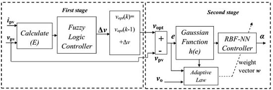
4. Proposed MPPT Based Fuzzy-Adaptive RBF-NN

In the literature, many methods have been designed in order to enhance the incremental conductance algorithm and to tackle the problem of oscillation around the MPP in the steady-state due to the fixed voltage-step-size (Δv). The following relationship is used in References [10,11] to vary the voltage-step-size:
Δ v ( k + 1 ) = M Δ p ( k ) Δ v ( k )
where Δp and Δv represent respectively the changes in PV-module power and PV-module voltage, while M is the scaling factor that requires tuning at each sample time to adjust the step size, which is proportional to the Δpv ratio.
In this section, we introduce the fuzzy logic to provide a variable voltage-step-size (Δv) in which, the overall MPPT control scheme of the proposed fuzzy adaptive RBF-NN is shown in Figure 8. The details of the second stage of the proposed MPPT controller have been previously given, and in the following, we give the reasons for what the fuzzy logic is used instead of INC algorithm in the first stage.
As it is adaptive in nature, the fuzzy logic controller intelligently varies the voltage-step-size to reduce steady-state oscillations. When the PV-system operating point is far from the MPP in the right plan or in the left plan, the voltage-step-size is made larger with a positive or negative value. As the PV-system operating point gets nearer to the MPP, the absolute voltage-step-size is dynamically reduced until it becomes very small.
The fuzzy logic controller uses the basis of the incremental conductance algorithm for the voltage-step-size regulation in order to ensure that the sum of the PV-module conductance and its incremental (G + ΔG) is zero at the MPP. The fuzzy logic controller has one input (E = G + ΔG) and one output (Δv), as shown in Figure 9.
The fuzzy subset partitions and shapes of the membership functions in the input and output depend on the behavior of the input and output of the controlled PV-system. After simulating the PV-system and plotting the controller input (E) versus PV-module voltage in Figure 10a, we can observe that when vpv is near to zero, the error E will tend to infinity. To avoid this problem, an initial value for vpv can be set, in which E will be included in the interval of [−1, 1]. The shapes and fuzzy subset partitions of the membership functions are given in Figure 10b, where the triangular membership function form is used for its easy computation and immediate solution to the optimization problems emerging in fuzzy modeling [62].
From Figure 10a, it can be seen that the maximum power point zone for the variable profile of irradiance is characterized for an error E around 0. Hence the membership functions for input E in Figure 10b, while taking into account this value, are constructed based on the following assumptions:
-
The absolute error E less than 0.25, it is considered as “the vopt zone (ZE)”.
-
The error E less than 0.5, it is considered as “near to vopt (PS) in the left half-plane”.
-
The error E bigger than 0.5, it is considered as “far from vopt in the left half-plane”. In this case, the trapezoidal membership function is used to saturate on (PB).
-
The same procedure when E is in the negative part (right half-plane).
-
The output Δv is defined in the common normalized range of [−0.3, 0.3]; −0.3 and 0.3 volts are considered as the maximum negative value and maximum positive value that can perturb the PV-module voltage. It is worth noting that increasing the search range helps the fuzzy controller to track the optimal voltage. However, an excessively wide range can cause a loss of power.
The fuzzy rules which associate the fuzzy output to the fuzzy input are derived from the knowledge of the system behavior in Figure 10a. The proposed method provides the operating region of the PV-module. If E > 0 (PB or PS), the operating point is located on the left half-plane of the ppv-vpv curve, the output voltage of the PV-module becomes small and the system must increase the voltage-step-size in order to achieve the optimal output voltage vopt. If E < 0 (NB or NS), the operating point is located on the right half-plane of the ppv-vpv curve, the output voltage of the PV-module becomes big and the system must decrease the voltage-step-size in order to achieve the optimal output voltage vopt. If E = 0, the operating point is at the MPP, so the voltage-step-size will be zero. Based on these concepts, the fuzzy rules database, which is divided into three regions, is obtained. Fuzzy rules are given in Table 2, in which NB denotes "negative big", NS denotes “negative small”, ZE denotes “zero”, PS denotes “positive small” and PB denotes “positive big”. The three regions are defined as follows:
Region 1: The operating point of the PV-module is located at the right half-plane of the ppv-vpv curve. The amount that the voltage step size is decreased depends on the distance between the operating point and the MPP.
Region 2: The operating point is close to the MPP. The voltage step size is thus equal to zero.
Region 3: The operating point of the PV-module is located at the left half-plane of the ppv-vpv curve. The amount that the voltage step size is increased depends on the distance between the operating point and the MPP.
The maximum of the minimum (Max–Min) composition technique of Mamdani has been used here for the inference. Moreover, the center-of-gravity method has been used for the defuzzification process that converts the fuzzy subset of the voltage-step-size to real numbers, as presented in the following equation:
Δ v = j = 1 n μ ( Δ v j ) Δ v j j = 1 n μ ( Δ v j )
where Δvj is the center of the Max–Min composition at the output membership function.
Remark 4. 
Compared to the conventional MPPT methods based on fixed step size with direct control like P and O and INC; the Fuzzy-adaptive RBF-NN consume considerable computation time; so the real-time implementation of it requires powerful CPU with big memory; so it becomes more computationally expensive. In contrast, the conventional approaches require only a few lines for the computer code which requires low CPU speed and short memory.

5. Simulation Results

In order to verify the effectiveness and robustness of the proposed fuzzy-adaptive RBF-NN control scheme, a comparative study with the classical perturb and observe method (P and O) [5] is provided. A fixed step-size of duty cycle Δα = 1 × 10⁻⁴ is used, and the following parameters of the RBF-NN have been chosen: hidden layer node m = 31, learning factor η = 0.001, momentum factor λ = 0.04, centric vector cj = [−15, −14, …., 14, 15]T, variance vector bj = 0.7 × ones (31,1) and initial weight vector wj (0) = 0.1 × rand (31,1).
The comparative study is carried out under four different scenarios: (1) standard climatic conditions (T = 25 °C and S = 1000 W/m2), (2) slope variation of irradiance, (3) step changes of the load R and 4) validation with a real profile of temperature and irradiance.
First scenario: In this case, the MPPT is performed under fixed values of temperature (T = 25 °C), irradiance (S = 1000 W/m2) and resistive load (R = 30 Ω). Figure 11a shows the tracking performance of the two MPPT algorithms, and Figure 11b shows the duty cycle of the boost converter. It can be seen that the proposed fuzzy-adaptive RBF-NN tracks perfectly the MPP without any oscillation and with a short rise time. On the other hand, the classical P and O presents oscillations at the steady-state (zoom 1 portion) which causes a significant loss of power.
Second scenario: In this case the MPPT is performed under a fixed value of temperature (T = 25 °C), a variable profile of irradiance shown in Figure 12 and a fixed value of the resistive load (R = 30 Ω). This profile of irradiance is generally used, e.g., References [9,12,20], to test the ability of MPPT controllers to deal effectively with slope variations of the irradiance. The irradiance is set to 600 W/m2 in the time interval [0 0.4] s, and to 400 W/m2 in the interval [1.3 1.5] s. In the interval [0.4 0.8] s, the irradiance increases from 600 to 1000 W/m2, and in the interval [1 1.3] s, the irradiance decreases from 1000 to 400 W/m2.
Figure 13a shows the simulation results of the PV-module power and Figure 13b of the duty cycle. It is observed that both MPPT strategies track the MPP, but performance degradation can be noticed when using the P and O control system. With irradiation changes, the MPP also changes its position, and so the controllers act in order to track the new MPP. Figure 13a shows that the proposed approach tracks the MPP almost perfectly, especially during the increase and the decrease of the irradiance. The oscillation around the MPP is null and our system never loses its tracking maximum power, while the P and O still presents oscillations when the MPP is reached, as shown in the zoom 2 portion. Furthermore, during the slope variation of the irradiance (ascending or descending), the P and O lost the direction of the maximum power tracking, as shown in the zoom 3 and zoom 4 portions.
Third scenario: The system is simulated under the sudden step resistive-load changes shown in Figure 14, with fixed values of irradiance (S = 1000 W/m2) and temperature (T = 25 °C). In Reference [63] the authors have given full details about the relationship between the MPPT technique and a variable resistive load.
Figure 15a shows simulation results of the PV-module power and Figure 15b of the duty cycle. It is observed that the proposed fuzzy adaptive RBF-NN outperforms the P and O algorithm in terms of their robustness. These figures show that an increase of R produces an increase of the duty cycle in order to track the MPP of the PV-module. In Figure 15a, when the resistive load (R) is suddenly increased from 10 Ω to 15 Ω at instant 4 s, the PV-module power using the P and O algorithm drops from Pmax = 61.92 watts to 51.19 watts and it takes about 0.1462 s to return to the Pmax. In the same figure, when R is increased from 15 Ω to 20 Ω at instant 6 s, the power drops to 56.96 watts and it takes 0.09 s to return to Pmax. On the contrary, these disadvantages are not present when our method is used. In this case, the duty cycle acts instantaneously when the value of the load R changes and the drop of the power is negligible.
Fourth scenario: In this case, the MPPT techniques are simulated using a real daily profile of irradiance and temperature as shown in Figure 16. The data of irradiance and temperature were measured in “Unité de Recherche Appliquée en Energies Renouvelable, in Ghardaïa, Algeria” on November 05, 2012 [64], using the K and Z CHP1 Pyrheliometer and Campbell CS21 tools. This choice allows us to assess the effect of using MPPT controllers in the PV system as well as the differences in performance existing among them. The changes in irradiance and temperature are almost proportional to the morning day time until 12:00 h. From 12:00 h to 15:00 h, the irradiance varies between 814 and 844 W/m2 and the temperature still increases until 33 °C, beginning from 30 °C at 12:00 h. After 15:00 h, the irradiance decreases until 160 W/m2 at 18:00 h while the temperature remains constant between 15:00 h and 17:00 h and decreases after that as a consequence of the sunset.
Figure 17a shows that the PV-module power generated with our proposed MPPT technique is greater than the power generated with the P and O algorithm. The main differences can be seen in the morning and the afternoon, when the irradiance and temperature increase or decrease. It can also be seen that the PV-module power curves obtained with the two MPPT controllers have an almost smooth curve, with the only exception that the P and O curve presents some oscillations when the irradiation becomes nearly constant, for example between 13:00 h and 15:00 h. The duty cycle curves plotted in Figure 17b show that the P and O is better than our method because it does not exhibit oscillations. To gain a deeper insight into this issue, the PV-module voltage is plotted in Figure 18a and the tracking error (e) in Figure 18b. Regarding the PV-module characteristics (Figure 3), the voltage decreases when the temperature increases; so the controller will act at each instant to regulate the PV-module voltage at its desired value (vopt). When the voltage drops, the controller tries to increase it in order to keep it at vopt. Subsequently, in the next instant, the voltage drops again because the temperature continues increasing and, then, the controller will increase the voltage again. This phenomenon will produce oscillations (or peaks) around the vopt. When the temperature is approximately constant, the oscillation is almost negligible. Due to the voltage drop produced at each instant, the error shown in Figure 18b is a consequence of the fact that the first stage of MPPT controller (fuzzy logic or other strategies) cannot perfectly track the vopt. It can be seen in Figure 18b that the amplitude of the error is comprised between −0.2 and 0.2 volts, which implies a maximum loss of 1% in vopt, that is considered a negligible value. The robustness of our method is also confirmed between 16:00 h and 18:00 h, when the P and O cannot keep the PV-module voltage at vopt while our method has the ability to almost keep the voltage at vopt. This is ensured by decreasing the duty cycle until it reaches its minimum value.
In order to carry out a comparison between the synthesized algorithms in all the considered tests, the performance index [12], given by the following equation:
η = i = 1 N p MPPT ( i ) i = 1 N p Max ( i ) × 100
is used. It is based on the efficiency calculated as the quotient between the output power of the photovoltaic system with the MPPT controller (PMPPT) and the output power at the true MPP (Pmax), in which N is the number of samples.
The results shown in Table 3 allow us to state that, in general, the proposed MPPT strategy with fuzzy adaptive RBF-NN offers the best performance (values in bold) compared with the INC adaptive RBF-NN and the conventional P and O algorithms. The INC adaptive RBF-NN strategy has shown its superiority over the P and O algorithm, demonstrating that the hybridization of intelligent and conventional controllers for MPPT can enhance the system performance.

6. Conclusions

In this article, a novel two-stage MPPT controller based on fuzzy adaptive RBF-NN has been proposed. In the first stage, a fuzzy logic system based on the concepts of incremental conductance algorithm has been used for the variable voltage-step-size calculation to reduce as much as possible the oscillations around the MPP. In the second stage, an RBF-NN has been used to provide the duty cycle of the boost converter to keep the PV-module voltage at the optimal voltage generated from the first stage. In order to track the real MPP in different atmospheric conditions and load variation, the backpropagation algorithm with gradient descent method has been proposed to learn the weights of the RBF-NN in order to minimize the mean-squared-error criterion.
Simulation results have shown the capability of our proposed MPPT controller to track the MPP without oscillations. The proposed approach has demonstrated its superiority in term of efficiency compared to the classical P and O and INC-adaptive RBF-NN.
The future work will focus on the real-time implementation of this proposed approach to validate it experimentally.

Author Contributions

The preparation of this work was involved by all the authors. conceptualization, N.B.; methodology, N.B., B.B. (Boualam Benlahbib) and B.B. (Bachir Batoun); software, B.B. (Boualam Benlahbib) and N.B.; validation, N.B., B.B. (Boualam Benlahbib), D.B., F.B. and V.F-B.; formal analysis, N.B.; investigation, N.B.; resources, N.B.; data curation, N.B. and B.B. (Boualam Benlahbib); writing—original draft preparation, N.B., B.B. (Boualam Benlahbib) and B.B. (Bachir Batoun); writing—review and editing, V.F-B.; visualization, B.B. (Bachir Batoun); supervision, D.B., F.B., V.F-B.; project administration, N.B.; funding acquisition, V.F-B.

Funding

This work has been financially supported in part by the Directorate-General for Scientific Research and Technological Development-Algerian Ministry of Higher Education and Scientific Research, in part by the University of Castilla-La Mancha under Project 2019-GRIN-26969 and in part by the European Social Fund (FEDER, EU).

Conflicts of Interest

The authors declare no conflict of interest.

References

  1. Liu, F.; Kang, Y.; Zhang, Y.; Duan, S. Comparison of P&O and hill climbing MPPT methods for grid-connected PV converter. In Proceedings of the 2008 3rd IEEE Conference on Industrial Electronics and Applications, Singapore, 3–5 June 2008; pp. 804–807. [Google Scholar]
  2. Yu, T.-C.; Lin, Y.-C. A study on maximum power point tracking algorithms for photovoltaic systems. Department of Electrical Engineering, Lunghwa University of Science and Technology (LHU) 2010, 30, 27–36. [Google Scholar]
  3. Hussein, K.; Muta, I.; Hoshino, T.; Osakada, M. Maximum photovoltaic power tracking: an algorithm for rapidly changing atmospheric conditions. IEE Proc.-Gener., Transm. Distrib. 1995, 142, 59–64. [Google Scholar] [CrossRef]
  4. Femia, N.; Petrone, G.; Spagnuolo, G.; Vitelli, M. Optimization of perturb and observe maximum power point tracking method. IEEE Trans. Power electron. 2005, 20, 963–973. [Google Scholar] [CrossRef]
  5. Ilyas, A.; Ayyub, M.; Khan, M.R.; Husain, M.A.; Jain, A. Hardware Implementation of Perturb and Observe Maximum Power Point Tracking Algorithm for Solar Photovoltaic System. Trans. Electr. Electr. Mater. 2018, 19, 222–229. [Google Scholar] [CrossRef]
  6. Berrera, M.; Dolara, A.; Faranda, R.; Leva, S. Experimental test of seven widely-adopted MPPT algorithms. In Proceedings of the 2009 IEEE Bucharest PowerTech, Bucharest, Romania, 28 June–2 July 2009; pp. 1–8. [Google Scholar]
  7. Ahmad, J. A fractional open circuit voltage based maximum power point tracker for photovoltaic arrays. In Proceedings of the 2nd International Conference on Software Technology and Engineering (ICSTE), San Juan, PR, USA, 3–5 October 2010; pp. 1–250. [Google Scholar]
  8. Noguchi, T.; Togashi, S.; Nakamoto, R. Short-current pulse-based maximum-power-point tracking method for multiple photovoltaic-and-converter module system. IEEE Trans. Ind. Electr. 2002, 49, 217–223. [Google Scholar] [CrossRef]
  9. Ishaque, K.; Salam, Z.; Lauss, G. The performance of perturb and observe and incremental conductance maximum power point tracking method under dynamic weather conditions. Appl. Energy 2014, 119, 228–236. [Google Scholar] [CrossRef]
  10. Pandey, A.; Dasgupta, N.; Mukerjee, A.K. Design issues in implementing MPPT for improved tracking and dynamic performance. In Proceedings of the IECON 2006-32nd Annual Conference on IEEE Industrial Electronics, Paris, France, 6–10 November 2006; pp. 4387–4391. [Google Scholar]
  11. Liu, F.; Duan, S.; Liu, F.; Liu, B.; Kang, Y. A variable step size INC MPPT method for PV systems. IEEE Trans. Ind. Electr. 2008, 55, 2622–2628. [Google Scholar]
  12. Ahmed, J.; Salam, Z. An improved perturb and observe (P&O) maximum power point tracking (MPPT) algorithm for higher efficiency. Appl. Energy 2015, 150, 97–108. [Google Scholar]
  13. Xu, Z.-R.; Yang, P.; Zhou, D.-B.; Li, P.; Lei, J.-Y.; Chen, Y.-R. An improved variable step size MPPT algorithm based on INC. J. Power Electr. 2015, 15, 487–496. [Google Scholar] [CrossRef]
  14. Mamarelis, E.; Petrone, G.; Spagnuolo, G. A two-steps algorithm improving the P&O steady-state MPPT efficiency. Appl. Energy 2014, 113, 414–421. [Google Scholar]
  15. Cheikh, M.A.; Larbes, C.; Kebir, G.T.; Zerguerras, A. Maximum power point tracking using a fuzzy logic control scheme. Rev. Des Energies Renouv. 2007, 10, 387–395. [Google Scholar]
  16. Algazar, M.M.; El-Halim, H.A.; Salem, M.E.E.K. Maximum power point tracking using fuzzy logic control. Int. J. Electr. Power Energy Syst. 2012, 39, 21–28. [Google Scholar] [CrossRef]
  17. Shiau, J.-K.; Wei, Y.-C.; Chen, B.-C. A study on the fuzzy-logic-based solar power MPPT algorithms using different fuzzy input variables. Algorithms 2015, 8, 100–127. [Google Scholar] [CrossRef]
  18. Bouarroudj, N.; Boukhetala, D.; Djari, A.; Rais, Y.; Benlahbib, B. FLC based Gaussian membership functions tuned by PSO and GA for MPPT of photovoltaic system: A comparative study. In Proceedings of the 2017 6th International Conference on Systems and Control (ICSC), Batna, Algeria, 7–9 May 2017; pp. 317–322. [Google Scholar]
  19. Ameur, K.; Ait-Cheikh, M.S.; Essounbouli, N. A PSO-based Optimization of a fuzzy-based MPPT controller for a photovoltaic pumping system used for irrigation of greenhouses. Iran. J. Fuzzy Syst. 2016, 13, 1–18. [Google Scholar]
  20. Larbes, C.; Cheikh, S.A.; Obeidi, T.; Zerguerras, A. Genetic algorithms optimized fuzzy logic control for the maximum power point tracking in photovoltaic system. Renew. Energy 2009, 34, 2093–2100. [Google Scholar] [CrossRef]
  21. Guenounou, O.; Dahhou, B.; Chabour, F. Adaptive fuzzy controller based MPPT for photovoltaic systems. Energy Convers. Manag. 2014, 78, 843–850. [Google Scholar] [CrossRef]
  22. Ishaque, K.; Salam, Z.; Amjad, M.; Mekhilef, S. An improved particle swarm optimization (PSO)–based MPPT for PV with reduced steady-state oscillation. IEEE Trans. Power Electr. 2012, 27, 3627–3638. [Google Scholar] [CrossRef]
  23. Ishaque, K.; Salam, Z.; Shamsudin, A.; Amjad, M. A direct control based maximum power point tracking method for photovoltaic system under partial shading conditions using particle swarm optimization algorithm. Appl. Energy 2012, 99, 414–422. [Google Scholar] [CrossRef]
  24. Dolara, A.; Grimaccia, F.; Mussetta, M.; Ogliari, E.; Leva, S. An Evolutionary-Based MPPT Algorithm for Photovoltaic Systems under Dynamic Partial Shading. Appl. Sci. 2018, 8, 558. [Google Scholar] [CrossRef]
  25. Duan, Q.; Mao, M.; Duan, P.; Hu, B. An intelligent algorithm for maximum power point tracking in photovoltaic system under partial shading conditions. Trans. Inst. Meas. Control 2017, 39, 244–256. [Google Scholar] [CrossRef]
  26. Ahmed, J.; Salam, Z. A Maximum Power Point Tracking (MPPT) for PV system using Cuckoo Search with partial shading capability. Appl. Energy 2014, 119, 118–130. [Google Scholar] [CrossRef]
  27. Mahmoud, A.; Tamer, K.; Mushtaq, N.; Mohd, A.A. An Improved Maximum Power Point Tracking Controller for PV Systems Using Artificial Neural Network. Przegląd Elektrotechniczny (Electr. Rev.) 2012, 88, 116–121. [Google Scholar]
  28. Sedaghati, F.; Nahavandi, A.; Badamchizadeh, M.A.; Ghaemi, S.; Fallah, M.A. PV maximum power-point tracking by using artificial neural network. Math. Probl. Eng. 2012. [Google Scholar] [CrossRef]
  29. Farayola, A.M.; Hasan, A.N.; Ali, A. Efficient photovoltaic MPPT system using coarse gaussian support vector machine and artificial neural network techniques. Int. J. Innov. Comput., Inf. Control (IJICIC) 2018, 14, 323–339. [Google Scholar]
  30. Khanaki, R.; Radzi, M.A.M.; Marhaban, M.H. Artificial neural network based maximum power point tracking controller for photovoltaic standalone system. Int. J. Green Energy 2016, 13, 283–291. [Google Scholar] [CrossRef]
  31. Kassem, A.M. MPPT control design and performance improvements of a PV generator powered DC motor-pump system based on artificial neural networks. Int. J. Electr. Power&Energy Syst. 2012, 43, 90–98. [Google Scholar]
  32. Zhang, L.; Bai, Y. On-line neural network training for maximum power point tracking of PV power plant. Trans. Inst. Meas. Control 2008, 30, 77–96. [Google Scholar] [CrossRef]
  33. Ghedhab, N.; Youcefettoumi, F. Optimized Photovoltaic Power Generator Using Artificial Neural Network Implementation for Maximum Power Point Tracking. Int. J. Environ. Sci. Dev. 2016, 7, 642. [Google Scholar] [CrossRef]
  34. Cheikh, M.A.; Haddadi, M.; Zerguerras, A. Design of a neural network control scheme for the maximum power point tracking (MPPT). Rev. des energies Renouv. 2007, 10, 109–118. [Google Scholar]
  35. Elobaid, L.; Abdelsalam, A.K.; Zakzouk, E.E. Artificial neural network based maximum power point tracking technique for PV systems. In Proceedings of the IECON 2012—38th Annual Conference on IEEE Industrial Electronics Society, Montreal, QC, Canada, 25–28 October 2012; pp. 937–942. [Google Scholar]
  36. Punitha, K.; Devaraj, D.; Sakthivel, S. Artificial neural network based modified incremental conductance algorithm for maximum power point tracking in photovoltaic system under partial shading conditions. Energy 2013, 62, 330–340. [Google Scholar] [CrossRef]
  37. Liu, Y.-H.; Liu, C.-L.; Huang, J.-W.; Chen, J.-H. Neural-network-based maximum power point tracking methods for photovoltaic systems operating under fast changing environments. Sol. Energy 2013, 89, 42–53. [Google Scholar] [CrossRef]
  38. Ranjani, K.; Raja, M.; Anitha, B. Maximum power point tracking by ANN controller for a standalone photovoltaic system. Int. J. Electr. Comput. Electron. Commun. Eng. 2014, 8, 592–596. [Google Scholar]
  39. Messalti, S.; Harrag, A.; Loukriz, A. A new variable step size neural networks MPPT controller: Review, simulation and hardware implementation. Renew. Sustain. Energy Rev. 2017, 68, 221–233. [Google Scholar] [CrossRef]
  40. Kofinas, P.; Dounis, A.I.; Papadakis, G.; Assimakopoulos, M. An Intelligent MPPT controller based on direct neural control for partially shaded PV system. Energy Build. 2015, 90, 51–64. [Google Scholar] [CrossRef]
  41. Abu-Rub, H.; Iqbal, A.; Ahmed, S.M. Adaptive neuro-fuzzy inference system-based maximum power point tracking of solar PV modules for fast varying solar radiations. Int. J. Sustain. Energy 2012, 31, 383–398. [Google Scholar] [CrossRef]
  42. Chaouachi, A.; Kamel, R.; Nagasaka, K. MPPT operation for PV grid-connected system using RBFNN and fuzzy classification. World Acad. Sci., Eng. Technol. 2010, 65, 97–105. [Google Scholar]
  43. Subiyanto, S.; Mohamed, A.; Hannan, M. Intelligent maximum power point tracking for PV system using Hopfield neural network optimized fuzzy logic controller. Energy Build. 2012, 51, 29–38. [Google Scholar] [CrossRef]
  44. Veerachary, M.; Senjyu, T.; Uezato, K. Neural-network-based maximum-power-point tracking of coupled-inductor interleaved-boost-converter-supplied PV system using fuzzy controller. IEEE Trans. Ind. Electr. 2003, 50, 749–758. [Google Scholar] [CrossRef]
  45. Belkaid, A.; Gaubert, J.P.; Gherbi, A. An improved sliding mode control for maximum power point tracking in photovoltaic systems. J. Control Eng. Appl. Inform. 2016, 18, 86–94. [Google Scholar]
  46. Chin, V.J.; Salam, Z.; Ishaque, K. Cell modelling and model parameters estimation techniques for photovoltaic simulator application: A review. Appl. Energy 2015, 154, 500–519. [Google Scholar] [CrossRef]
  47. Romero, B.; Del Pozo, G.; Arredondo, B. Exact analytical solution of a two diode circuit model for organic solar cells showing S-shape using Lambert W-functions. Sol. Energy 2012, 86, 3026–3029. [Google Scholar] [CrossRef]
  48. Ahmad, T.; Sobhan, S.; Nayan, M.F. Comparative analysis between single diode and double diode model of PV cell: concentrate different parameters effect on its efficiency. J. Power Energy Eng. 2016, 4, 31. [Google Scholar] [CrossRef]
  49. Shannan, N.M.A.A.; Yahaya, N.Z.; Singh, B. Single-diode model and two-diode model of PV modules: A comparison. In Proceedings of the 2013 IEEE International Conference on Control System, Computing and Engineering, Mindeb, Malaysia, 29 November–1 December 2013; pp. 210–214. [Google Scholar]
  50. Duong, M.Q.; Nguyen, H.; Leva, S.; Mussetta, M.; Sava, G.N.; Costinas, S. Performance analysis of a 310Wp photovoltaic module based on single and double diode model. In Proceedings of the 2016 International Symposium on Fundamentals of Electrical Engineering (ISFEE), Bucharest, Romania, 30 June–2 July 2016; pp. 1–6. [Google Scholar]
  51. AlRashidi, M.; El-Naggar, K.; AlHajri, M. Parameters estimation of double diode solar cell model. Int. J. Electr. Comput. Energ. Electr. Commun. Eng. 2013, 7, 118–121. [Google Scholar]
  52. Ait-Cheikh, M.S. Etude, Investigation et conception d’algorithmes de commande appliqués aux systèmes photovoltaïques. Ph.D. Thesis, Ecole Nationale Polytechnique, Algiers, Algeria, December 2007. [Google Scholar]
  53. Yordanov, G.; Midtgård, O.; Saetre, T. Two-diode model revisited: Parameters extraction from semi-log plots of I-V data. In Proceedings of the 25th European Photovoltaic Solar Energy Conference and Exhibition/5th World Conference on Photovoltaic Energy Conversion, Valencia, Spain, 6–10 September 2010; pp. 4156–4163. [Google Scholar]
  54. Franzitta, V.; Orioli, A.; Gangi, A.D. Assessment of the Usability and Accuracy of Two-Diode Models for Photovoltaic Modules. Energies 2017, 10, 564. [Google Scholar] [CrossRef]
  55. Bechouat, M.; Younsi, A.; Sedraoui, M.; Soufi, Y.; Yousfi, L.; Tabet, I.; Touafek, K. Parameters identification of a photovoltaic module in a thermal system using meta-heuristic optimization methods. Int. J. Energy Environ. Eng. 2017, 8, 331–341. [Google Scholar] [CrossRef] [Green Version]
  56. Et-torabi, K.; Nassar-eddine, I.; Obbadi, A.; Errami, Y.; Rmaily, R.; Sahnoun, S.; Agunaou, M. Parameters estimation of the single and double diode photovoltaic models using a Gauss–Seidel algorithm and analytical method: A comparative study. Energy Convers. Manag. 2017, 148, 1041–1054. [Google Scholar] [CrossRef]
  57. Ovaska, S. Maximum power point tracking algorithms for photovoltaic applications. Master’s Thesis, Aalto University, Espoo, Finland, 14 December 2010. [Google Scholar]
  58. Ogliari, E.; Dolara, A.; Manzolini, G.; Leva, S. Physical and hybrid methods comparison for the day ahead PV output power forecast. Renew. Energy 2017, 113, 11–21. [Google Scholar] [CrossRef]
  59. Fei, J.; Wang, Z. Adaptive RBF neural network control for three-phase active power filter. Int. J. Adv. Robot. Syst. 2013, 10, 258. [Google Scholar] [CrossRef]
  60. Widrow, B.; Lehr, M.A. 30 years of adaptive neural networks: perceptron, madaline, and backpropagation. Proc. IEEE 1990, 78, 1415–1442. [Google Scholar] [CrossRef]
  61. Rumelhart, D.E.; Hinton, G.E.; Williams, R.J. Learning internal representations by error propagation; Institute for Cognitive Science, University of California: Oakland, CA, USA, September 1985. [Google Scholar]
  62. Pedrycz, W. Why triangular membership functions? Fuzzy sets Syst. 1994, 64, 21–30. [Google Scholar] [CrossRef]
  63. Al-Gizi, A.G. Comparative study of MPPT algorithms under variable resistive load. In Proceedings of the 2016 International Conference on Applied and Theoretical Electricity (ICATE), Craiova, Romania, 6–8 October 2016; pp. 1–6. [Google Scholar]
  64. Bechouat, M.; Soufi, Y.; Sedraoui, M.; Kahla, S. Energy storage based on maximum power point tracking in photovoltaic systems: A comparison between GAs and PSO approaches. Int. J. Hydrog. Energy 2015, 40, 13737–13748. [Google Scholar] [CrossRef]
Figure 1. Principal chain of a photovoltaic system with an MPPT controller.
Energies 12 02827 g001
Figure 2. Two-diode electrical model of PV cell.
Energies 12 02827 g002
Figure 3. (a) ppv-vpv-module characteristic, (b) ipv-vpv-module characteristic for different irradiance and temperature levels.
Energies 12 02827 g003
Figure 4. Circuit of the DC-DC boost converter.
Energies 12 02827 g004
Figure 5. Mechanism of searching maximum power point.
Energies 12 02827 g005
Figure 6. Scheme of proposed MPPT controller-based INC-adaptive RBF-NN.
Energies 12 02827 g006
Figure 7. (a) Sign of G + ΔG for different zones of operation in ppv-vpv curve, (b) optimal voltage searching algorithm [3,57].
Energies 12 02827 g007
Figure 8. The structure of proposed fuzzy adaptive RBF-NN for MPPT.
Energies 12 02827 g008
Figure 9. Fuzzy logic controller (FLC) for calculating Δv.
Energies 12 02827 g009
Figure 10. (a) Behavior of FLC input and output, (b) Membership function for input and output of FLC.
Energies 12 02827 g010
Figure 11. (a) PV-module power. (b) Duty cycle under standard climatic conditions.
Energies 12 02827 g011
Figure 12. Slope variation of irradiance.
Energies 12 02827 g012
Figure 13. (a) PV-module power. (b) Duty cycle under slope variation of irradiance.
Energies 12 02827 g013
Figure 14. Load step changes.
Energies 12 02827 g014
Figure 15. (a) PV-module power. (b) Duty cycle under load step changes.
Energies 12 02827 g015
Figure 16. Real daily profile of (a) irradiance and (b) temperature.
Energies 12 02827 g016
Figure 17. (a) PV-module power. (b) Duty cycle under the real profile of temperature and irradiance.
Energies 12 02827 g017
Figure 18. (a) PV-module voltage. (b) Input error of RBF-NN under the real profile of temperature and irradiance.
Energies 12 02827 g018
Table 1. Specifications used for the PV-module [52].
ParametersValues
Maximum power Pmax61.92 W
Open Circuit Voltage voc25.25 V
Short Circuit Current iph-max3.25 A
Voltage at Maximum Power vopt20 V
Current at Maximum Power iopt3 A
Ideality factor n11
Ideality factor n22
Number of series cells Ns36
Table 2. Rules of the used fuzzy logic controller.
Region 1Region 2Region 3
Input ENBNSZEPSPB
Output ΔvNBNSZEPSPB
Table 3. A comparative study based on the performance index η.
P and OINC Adaptive RBF-NNFuzzy Adaptive RBF-NN
Scenario 196.2696.8798.13
Scenario 297.0398.5699.21
Scenario 389.5097.3899.14
Scenario 494.8997.7498.75

