Application of Machine Learning in Transformer Health Index Prediction


1
Mechanical Engineering Department, École de technologie supérieure, Montréal, QC H3C 1K3, Canada
2
Electrical and Computer Engineering, University of Waterloo, Waterloo, ON N2L 3G1, Canada
*
Author to whom correspondence should be addressed.
Energies 2019, 12(14), 2694; https://doi.org/10.3390/en12142694
Submission received: 18 June 2019
/
Revised: 10 July 2019
/
Accepted: 12 July 2019
/
Published: 14 July 2019
(This article belongs to the Special Issue High Voltage Engineering and Applications)
Abstract
:The presented paper aims to establish a strong basis for utilizing machine learning (ML) towards the prediction of the overall insulation health condition of medium voltage distribution transformers based on their oil test results. To validate the presented approach, the ML algorithms were tested on two databases of more than 1000 medium voltage transformer oil samples of ratings in the order of tens of MVA. The oil test results were acquired from in-service transformers (during oil sampling time) of two different utility companies in the gulf region. The illustrated procedure aimed to mimic a realistic scenario of how the utility would benefit from the use of different ML tools towards understanding the insulation health index of their transformers. This objective was achieved using two procedural steps. In the first step, three different data training and testing scenarios were used with several pattern recognition tools for classifying the transformer health condition based on the full set of input test features. In the second step, the same pattern recognition tools were used along with the three training/testing scenarios for a reduced number of test features. Also, a previously developed reduced model was the basis to reduce the needed number of tests for transformer health index calculations. It was found that reducing the number of tests did not influence the accuracy of the ML prediction models, which is considered as a significant advantage in terms of transformer asset management (TAM) cost reduction.
1. Introduction and Background
One of the major parameters that define the operation and planning of an electrical utility is the transformer asset health condition. Based on their health condition, electrical utility engineers can predict the transformer useful remnant lifetime. Such an understanding can benefit utility companies to prepare a proper financial plan to estimate the future cost of maintenance and replacement for the transformer units. Significant research has been conducted to help utility companies in cutting their asset maintenance costs. This area of research is commonly referred to as the transformer asset management (TAM) practice [1]. TAM, as explained in [1,2,3], defines a strategic set of future maintenance and replacement activities for the utility transformer asset based on diagnostic testing methods of the transformer health condition. The ultimate objective of TAM is to ensure the power system reliability within an economic platform. Abu-Elanien in [2] defines the diagnostic testing methods in its two-part forms of condition monitoring (CM) and condition assessment (CA). CM refers to all the electrical, chemical, and physical tests that are used collectively towards CA tools that determine the transformer health condition. Azmi et al. states that TAM practices are at their best when they are comprised of both the CA and financial information [3]. Having knowledge of the transformer history (loading and failure history), associated risk index (based on the load it feeds), current health condition, and all related financial costs (maintenance, operation, and failure) would result in an economic risk management plan with adequate subsequent decisions.
1.1. Insulation Health Index Computation
According to the literature, the transformer health condition is governed by its oil-paper insulation condition [1,4,5]. According to [1], analyzing the transformer oil samples would be more advantageous than testing other transformer components (turns ratio, winding resistance, leakage reactance, etc.) for fault detection and life expectancy. With the health condition of all transformer components being taken into consideration, the overall health condition can be defined using the health index (HI). The health index, as explained by Jahromi et al. [6,7], is a single index factor which combines operating observations, field inspections, and laboratory tests to aid in the TAM cycle. The insulation condition is a vital part of the HI computation that could suffice when limited data is available for the transformer service record and design. Understanding the insulation condition would require thorough transformer oil sample analysis through electrical, chemical, and physical laboratory tests.
All conducted oil insulation laboratory tests fall into one of three major test categories, which are namely the dissolved gases (DGA), oil quality (OQA), and furan (FFA) tests [6,7]. DGA tests are typically conducted for the detection of transformer internal faults (electrical and/or thermal). The dissolved gases include hydrogen (H2), methane (CH4), ethane (C2H6), ethene (C2H4), ethyne (C2H2), carbon monoxide (CO), and carbon dioxide (CO2) [8]. For the second category of tests, OQA, the oil quality is determined by testing the oil breakdown voltage (BDV), acidity, water content, interfacial tension (IFT), dielectric dissipation factor (DDF), and color [9]. Finally, the measurement of FFA determines the extent of paper insulation degradation through determining the furfuraldehyde (or commonly known as furan) content in the transformer oil. Furan is a chemical compound that dissolves in the insulation oil upon the breakdown of the cellulose chain of the paper material [10]. The furan test is a strong indicator of transformer paper insulation ageing. Collectively, laboratory tests on dissolved gases, oil, and paper quality would be used to compute the HI value based on a given formula that is developed by experts in the TAM field. Examples of such different formulas can be found in [6,7,8,9,10,11,12,13], with the method illustrated in [6,7] being solely used for computing the HI for the majority of publications.
1.2. Novel Methods for HI Computation
The approach of using artificial intelligence tools, such as machine learning (ML) technologies and fuzzy logic for the HI computation, was well studied in several publications. In Ref. [14], the assessment of the HI was done using a neuro-fuzzy approach. The aim of the study was to test the performance of the five-layer based neuro-fuzzy model in computing the HI as per the scoring method dictated in [6]. The inputs to the model were the oil test features that have been taken from in-service transformers records. Though limited in the number of available data, the author was able to show a prediction accuracy of more than 50% using the developed neuro-fuzzy model. In other works, such as [15], a general regression neural network (GRNN) was developed for the HI of four-class based condition assessment (namely, very poor, poor, fair, and good). For this particular work, the transformer health was graded based on international oil assessment standards (such as that of [9]). Six key inputs, including the oil total dissolved combustible gas, furan content, dielectric strength, acidity, water content, and dissipation factor, were utilized. An 83% success was reported in predicting the transformer health condition. Zeinoddini-Meymand et al. in [16] used an artificial neural network and neuro-fuzzy models to include the basic oil assessment test features and additional economical parameters that have not been accounted for in many publications. These economical parameters include the transformer percentage economical life-time and ageing acceleration factor. According to [16], the inclusion of such parameters in the HI condition-class problem resulted in an excellent assessment performance, which correlated with that of the field experts.
In the work of [17], probabilistic Markov chain models were used in predicting the future performance of the transformer asset based on their HI computation for a defined span of time. Transition probabilities have been derived (using a non-linear optimization technique) to be the core element of the Markov chain model, which in turn was used to predict the future HI of the transformer asset. The reported results indicate satisfactory prediction performances for a number of tested transformers. An interesting approach was presented by Tee et al. in [18] for determining the transformer health condition using principle component analysis (PCA) and analytical hierarchy process (AHP). Data of the transformer oil quality tests and age have been used in both the aforementioned techniques to rank the transformer asset based on the insulation health condition. The ranking obtained by both techniques showed a comparable performance to that of an expert-based empirical formula assessment for the same transformer asset.
In Ref. [19], a fuzzy-based support vector machine (SVM) was used in HI-condition assessment. The HI condition of a given transformer was determined based on a number of factors, including industry standards and utility expert judgments. The SVM model showed a classification rate of 87.8%. A fuzzy-logic based model was also incorporated in [20], where the HI class condition (three classes) was predicted using the technical oil test features as inputs. In other attempts, such as [21], a general study was conducted using different conventional feature selection methods on oil test features for predicting the HI condition with different ML techniques.
With reference to all the reported works in this paper, a promising future is foreseen for the use of ML in the TAM field. As was indicated earlier, predicting the HI of the transformer asset will substantially impact the financial strategy of the utility company in asset maintenance plans. The objective of this work was to extend our previous research of [22] and establish a platform for using a wide range of ML tools in understanding the transformer health condition.
1.3. Organization of the Presented Work
In the following sections of this paper, the transformer databases used for this study will be introduced. The methodology of computing the HI value and accordingly classifying the health condition for a given sample in the oil databases are illustrated. Thereafter, the different ML tools used in the pattern recognition/classification problem of this study are introduced. The stepwise regression feature selection tool will also be introduced. Accordingly, two major steps will be done in achieving the objectives of the presented work:
- Full-feature modelling: The pattern recognition model will be trained and tested based on the complete number of available test features (which is 10 in this study). Eight different pattern recognition methods will be used with three different training and testing scenarios based on the two different oil databases that were acquired in this study.
- Reduced-feature modelling: Based on the reported work of [22], stepwise regression was used as a feature selection tool for predicting the HI value of a given oil sample. Accordingly, it was concluded which oil test features are of the highest statistical significance in computing the HI value of a given transformer. Only the indicated oil test features from [22] will be used from the two databases in a reduced-feature modelling step. Again, eight different pattern recognition methods will be used along with the same three training and testing scenarios used in the full-feature modelling procedure.
2. Materials and Methods
2.1. Transformer Oil Samples
As mentioned earlier, transformer oil sample databases were acquired from two utility companies in the gulf region. For confidentiality purposes, the two companies will be referred to as Util1 and Util2. In total, 730 transformer oils samples were obtained from Util1, while 327 transformer oil samples were obtained from Util2. Transformers from both databases are medium voltage distribution transformers. Util1 transformers are 66/11 kV, 12.5 to 40 MVA, while those of Util2 are 33/11 kV and 15 MVA. For every transformer in both databases, 10 different oil test results are available, namely: H2, CH4, C2H6, C2H4, C2H2, BDV, IFT, water content, acidity, and furan.
2.2. Structuring the HI Database
The transformer databases have a total of 1057 data samples combined. The prime objective of this paper is to be able to estimate the transformer insulation health condition using ML with either the entire oil feature set or a partial part of it. The published work in [6,7] is considered as the base method for computing the HI. In this method, all input test features are assigned a score value based on a predefined scale. The scored test feature is then multiplied or scaled by a predefined weight factor and is quantifiably added to the other scaled test features. With the inclusion of other arithmatic operations, three quantitative factors related to the DGA, OQA, and FFA tests are calculated (denoted by ). The factors are discrete values that range from 1 to 5 (or 1 to 4 for ), with the ascending order of the values indicating a deteriorating condition of the transformer health. The three factors will then be multiplied by their associated weights (denoted by α) to eventually produce the HI value using Equation (1) as illustrated in [6]:
The HI value ranges from 0% to 100%, with 100% being a transformer in the healthiest possible condition. Once the HI is computed, the data sample is classified into one of three health condition classes, which are: Bad (B), fair (F), and good (G). Table 1 illustrates the HI value range for a given class and the number transformers from each utility company in that class.
To have a better visualization of the 10 input variables and how they are related to the health condition of the transformer data, a 3-D plot of the data using the factors from Equation (1) is depicted in Figure 1. As can be seen in Figure 1, there is a clear and distinct difference between the three classes of data that is influenced by the three factors.
2.3. The Machine Learning Methodology
Transformer condition assessment requires the analysis of substantial data, whose instances represent investigated transformers and whose features represent variables measured to predict the transformer HI condition. A pattern recognition or classification model (classifier) can be trained on the dataset so that learning algorithms can operate faster and more effectively; in other words, costs are reduced, and learning accuracy is improved [23]. The methodology presented in this paper is based on feature selection and pattern classification for assessing the HI of power transformers. ML helps in gaining insights into the properties of data dependencies, and the significance of individual attributes in the dataset. Classification is an ML technique used to assign labels (classes) to unlabeled input instances based on discriminant features. Class labels in this study are the three health condition classes. Feature selection techniques determine the important features to include in the classification process of a particular data collection. Ten features are available for this study as was illustrated earlier. The entire process of applying these ML techniques to predict the class of unseen data consists of the typical phases of training and testing.
Consider a binary classification problem with positive (P) and negative (N) classes (i.e., two class problem). As a generalization for such multi-class classification problems, the overall classification accuracy measure is assessed in terms of the quantity of truly and falsely classified samples. Accordingly, a confusion matrix is constructed for recording the frequency of truly positive (TP), truly negative (TN), falsely positive (FP), and falsely negative (FN) samples. Table 2 shows a confusion matrix for binary classification problems, in which the class is either P or N.
As illustrated in [24], the overall classification accuracy measure is calculated by:
To validate the classification model, the k-fold cross-validation technique is used. Wherein, the dataset is randomized then equally subdivided into k subsets, of which k − 1 subsets are used for training and the remaining subset is retained for testing to validate the resulting model. Then, a different subset is used as a test set and the remaining k − 1 are used for training; thus, a second model is built. The process is repeated k times (folds) until k models are built. The final estimation is based on the average of the k results. A 10-fold cross-validation is usually used [25]. This method has the advantage of using all data for both the testing and validation. Moreover, it reduces the standard deviation with random seeds, as compared to methods that split the dataset into two sets, a training set and a testing set.
Feature selection is the process of selecting a subset of relevant, high quality, and non-redundant features for building learning models [26], with improved accuracy [27]. Quite often, datasets contain features with different qualities, which can influence the performance of the entire learning framework. For instance, noisy features can decrease the classifiers’ performance. Moreover, some features are redundant and are highly correlated, i.e., they do not give additional information. Considering all available information, provided by all kinds of features, would make it hard for the classifier to discover the real distinguishing characteristics, and would cause it to be overly specified (over fitted) on the examples it is trained with, hence reducing its generalization power drastically. Therefore, it is important to select the appropriate features to base classification on them [28,29]. As explained in the earlier publication of [22] and detailed in [30], stepwise regression deals with studying the statistical significance of a number of test features as they relate to the variable of interest. In other words, stepwise regression will be used to determine which of the 10 oil test features will be adequately sufficient to predict the HI value with the absence of the least significant ones. In the stepwise regression process, a final multilinear regression model is developed for predicting the variable of interest by adding or removing test features in a stepwise manner. The process starts with a single feature present in the regression model. A feature is then added to assess the incremental performance of model in computing the variable of interest (the HI value in this case). In each step, the F-statistic of the added feature in the model is computed. The F-statistic is found by:
where is the regression coefficient of the associated feature in the multilinear regression model. Fj is the F-statistic value with the inclusion of the jth term in the regression model given the other existing test features in the model. SSR is the regression sum of squares of the data sets’ computed model output as compared to data sets’ actual values, and MSE is the mean square of error of the model with all its existing and currently tested features. During each step, a p-value for the F-statistic of the added feature is determined and tested against the null hypothesis. The null hypothesis rejects the idea that the feature in question is statistically significant to the variable of interest. Thus, when performing the stepwise feature selection in the forward manner and the p-value of the added term to the model is found to be below the pre-defined entrance tolerance, the null hypothesis is rejected and the term is added to the model. Once all the forward stepwise process is done, the stepwise process starts to move in the backward manner. If a given test feature that exists in the model has its p-value for the F-statistic above the exit tolerance, the null hypothesis is confirmed and that feature is removed from the final model.
2.4. Classifiers Used in the Study
In this paper, WEKA version 3.8.2 was used as the platform for the different classifiers. It is a collection of machine learning algorithms for data mining tasks developed at the University of Waikato, New Zealand. A brief description of the different machine learning algorithms used by WEKA in this study is presented below.
- Random Forest (RForest): It is a form of the nearest neighbor predictor that starts with a standard ML technique called a decision tree [31,32]. RForest is a meta-estimator that fits a number of decision tree classifiers on various sub-samples of the dataset and uses averaging to improve the predictive accuracy and control over-fitting. RForest is a fast classifier that can process many classification trees [22].
- Decision Tree (J48): J48 is the Java implementation of the C4.5 decision tree algorithm in the WEKA data mining software [32]. The algorithm builds decision trees by calculating the information gain of the attributes, and then uses the attribute that has the highest normalized information gain to split the instances into subsets of the same class label (called a leaf node of the tree). The algorithm repeats the same process with all split subsets as children of a node. Finally, the tree is pruned by removing the branches that do not help in classification.
- Support Vector Machines (SVMs): SVM classifies instances by constructing a set of hyperplanes to separate the class categories [33]. SVMs belong to the general category of kernel methods [34,35], which depend on the data only through dot products. To ensure that the hyperplane is as wide as possible between classes, the kernel function computes a projection product in some possibly high dimensional feature space. SVMs have the advantages of being less computationally intense than other classification algorithms, a good performance in high-dimensional spaces, and efficiency in handling nonlinear classification using the kernel trick that indirectly transforms the input space into another high dimensional feature space.
- Artificial Neural Networks (ANNs): ANNs are bio-inspired methods of data processing that enable computers to learn similarly to human brains [24]. ANNs are typically structured in layers made up of a number of interconnected nodes. Patterns are presented to the network via the input layer, which communicates to one or more hidden layers where the actual processing is done via a system of weighted connections. The hidden layers then link to an output layer where the answer (health index level in our case) is the output. In the learning phase, weights are changed until the best ANN model that fits the input data is built [24].
- k-Nearest Neighbor (kNN): The kNN algorithm is a supervised learning technique that has been used in many ML applications. It classifies objects based on the closest training examples in the feature space. The idea behind kNN is to find a predefined number of training samples closest in distance to a given query instance and predict the label of the query instance from them [24]. kNN is similar to a decision tree algorithm in terms of classification, but instead of finding a tree, it finds a path around the graph. It is also faster than decision trees.
- OneR: One rule is made for each attribute in the predictor variable in the dataset in which a given class is assigned to the value of that attribute [36]. The rule is created by counting the frequency of target classes that appear for a given attribute in the predictor variable. The most frequent target class is assigned for that attribute and the error for using that one rule for the entire data set is computed. The attribute of the predictor variable with the least error is considered as the final one rule. For the problem in this study, the attributes of each predictor variable are continuous numerical values and thus they must be discretized to create the one rule. The discretization process is thoroughly explained in [36].
- Multinomial Logistic Regression (MLR): A linear regression model attempts to fit a linear equation that maps the predictor variables to an estimated response variable [37]. Logistic regression or binary logistic regression, on the other hand, is more of a two-class classification-based model that is considered as a generalized linear model. The algorithm aims to define linear decision boundaries between the different classes [38]. The linear logistic regression model maps the input feature vector into a probability value via the sigmoid logistic function that is set during the training process. Based on the obtained probability, a decision is made of whether the given sample belongs to a particular class or not. For multiple classes, the MLR model is developed, which is a set of binary logistic regression models of a given class against all other classes. The classification of the sample is based on the maximum computed probability amongst the different logistic regression models [39].
- Naïve Bayes (NB): The NB classifier is a probabilistic classifier that is based on Bayes theorem [40]. This classifier is based on the assumption that the predictor variables are conditionally independent given the class of the data sample in question. In other words, the posterior probability of the sample being in a particular class given the predictor variables is computed using Bayes theorem [40]. For that, the likelihood of the predictor variable given the class, predictor prior probability, and class prior probability are determined. The samples are classified based on the outcome of the maximum posterior probability computed amongst all the different classes. This type of classifier is easily modelled and is typically suitable for large datasets.
3. Results
As illustrated earlier, two subsequent procedural steps were followed to achieve the main objective of this paper. In the first step, eight different classifiers were modelled for classifying the transformer health condition as being B, F, or G with three different training/testing scenarios involving the two utility databases (Util1 and Util2). The full number of 10 features (as obtained from Util1 and Util2) will be used to model the classifiers, and thus such classifiers will be named as the full-feature classifiers. In the following step, predetermined stepwise regression features from the reported results of [22] were used as the only features in modelling the eight classifiers with the same three training/testing scenarios of the full-feature model. Such classifiers will be named as the reduced-feature classifiers. An assessment of the performance of both the full-feature and reduced feature classifiers was done by means of the accuracy rate obtained as per Equation (2). The mean accuracy rate (MAR) is shown in the presented results, which is basically the average value obtained for the accuracy rate for 10 trials.
3.1. Full-Feature Classifier Modelling
Eight different types of classifiers were used, which are NB, MLR, ANN, SVM, kNN, OneR, J48, and RF. Different training and testing scenarios were designed for the study. For a training/testing scenario, Tr-Util1, Ts-Util1, the classifier would be trained on data from Util1 and tested using the unused data from Util1. Similarly is the case with a training/testing scenario, Tr-Util2, Ts-Util2.
In order to validate the generalized nature of the classifiers, a training/testing scenario, Tr-Util1, Ts-Util2, would have the classifier being trained on data from Util1 and tested on different data from Util2.
To have a better understanding of how the results are obtained, consider the following example. When applying the training/testing scenario Tr-Util1, Ts-Util1 with the RF classifier, the confusion matrix will indicate the frequency of truly and falsely classified data samples. Table 3 shows the confusion matrix obtained for the Tr-Util1, Ts-Util1 scenario using the RF classifier. As can be seen in Table 3, 99.2% (492 of 496) for the G class of transformers were correctly classified. Similarly, 94.2% and 68% of the data samples were correctly classified as the F and B class, respectively. The accuracy rate was calculated using Equation (2) as:
where TG, TF, and TB are the truly classified data samples in the G, F, and B classes, respectively, and FG, FF, and FB are the falsely classified data samples in the G, F, and B classes, respectively. The same simulation was done 10 times and the MAR was noted. Table 4 shows the summary of the obtained MAR results for eight classifier types with the three training/testing scenarios.
3.2. Reduced-Feature Classifier Modelling
In the published work of [22], it was concluded that the four test features of furan, IFT, C2H6, and C2H2 are the concise test features of the highest statistical significance in the regression problem of the HI value. The approach presented in this paper differs than that of [22] such that the ML approach deals with the prediction of the health condition class rather than the HI value (thus a classification problem rather than regression). Thus, the indicated four test features in [22] were used in the reduced-feature classifier modelling. Similar to the approach followed in the full-feature classifier models, eight classifiers with three different training/testing scenarios were used. Table 5 shows the summary of the obtained results for the MAR.
4. Discussions of the Results
Table 4 and Table 5 summarize the results obtained for more than 640 simulations combined. This section of the paper will highlight the most important results that would significantly support the objective of using ML for the transformer health index problem.
4.1. Full-Feature Classifier Results
With reference to Table 4, the following points should be noted:
- The overall MAR results obtained for the full-feature classifier models were above 85%. It was observed that the highest classification error was observed for the B class samples. Though many data samples that actually belong to the B class were misclassified, they were always misclassified as being in the F class rather than the G class. This sort of error is of minimal risk in the sense that the classifiers would never give a misleading information of the transformer being in an excellent health condition while truly being in the worst health condition. Table 6 shows examples of the confusion matrices obtained in which a significant number of the B samples were misclassified as being F samples. The misclassification in most cases is attributed to the fact that a limited number of transformer oil samples of the B class are available for training (only 33 samples in total as can be observed in Table 1).
- For the remaining health condition classes, the accuracy rate was high and acceptable for most simulations. Most of the classifiers performed well in distinguishing between an F sample and a G sample. This is mainly attributed to the fact that a significant number of samples are available from both classes for training data.
- One of the extremely important training/testing scenarios would be that of Tr-Util1, Ts-Util2. With reference to Table 4, it was observed that most of the classifiers for this particular scenario did not perform as well as in the other training/testing scenarios. This inferior performance is mainly attributed to the fact that the classifier training was done with data from one utility company and testing was done with completely unseen data from another utility company. Still, the MAR results obtained are excellent given the previously unseen testing data. The MLR and ANN classifiers were the best classifiers, which resulted in an MAR of 95.4%. These excellent results support the generalized nature of the proposed approach in such a way that a utility company can use pre-modelled classifiers for their own transformer oil samples.
4.2. Feature-Reduced Classifier Results
The selected features are basically the furan (which is an indicator of the paper insulation condition), the IFT (which is an indicator for the oil quality), and C2H2 and C2H6 that reveal the presence of any faults inside the transformer. Also, the ML can detect any correlation between the tests and hence remove highly correlated tests. With reference to Table 5, the obtained MAR results using most of the feature-reduced classifiers were above 90%. Similar to the full classifier models, the J48 and RF classifiers had the best performance amongst the eight reduced classifier models. These results give a significant conclusion that the feature selection technique of stepwise regression was very successful. The impact of these results would help utility companies reduce the cost of performing TAM practices by reducing the number of test samples required for computing the health index of the transformer asset. However, it is important to note that the frequency of oil sampling and hence overall TAM planning will not be improved by the results of the presented paper.
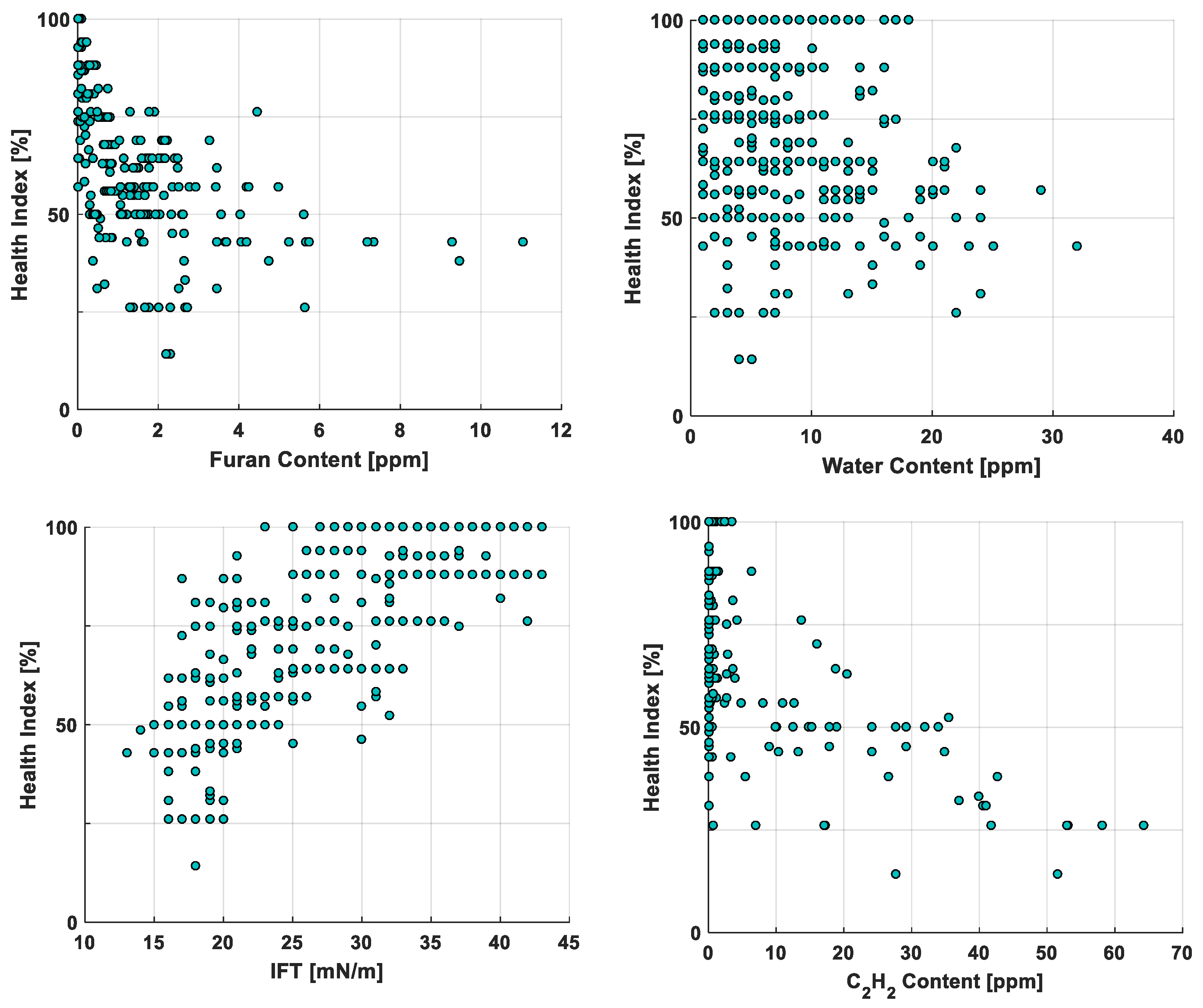
To illustrate the correlation of the health index with the selected features, Figure 2 shows the plots obtained for the furan, water, IFT, and C2H2 content against the health index. Although, furan, IFT, and C2H2 were selected by the stepwise regression, the water content was not selected [22]. Water clearly had the least correlation with the health index value, which would explain why it was not selected in either stepwise regression. On the other hand, the other three selected features showed a strong correlation with the health index.
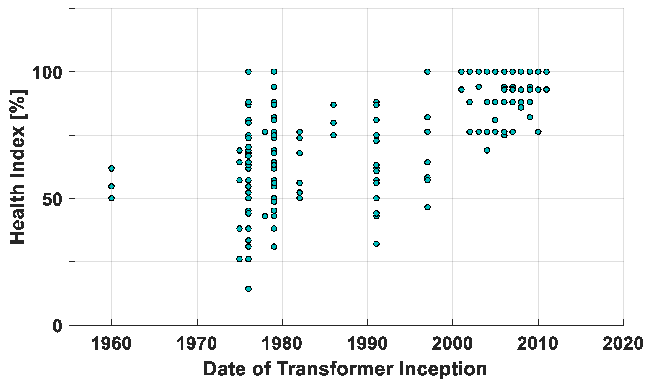
An additional study was conducted to observe if the age of the transformer was correlated with the obtained health index value. The age factor was not included in the study due to the fact that the transformer age data was only available for the transformer asset of Util1. Figure 3 shows the relationship between the transformer energization date and the health index value. It is apparent that there is no strong correlation between the transformer age and health index value. Merely, the transformer age may not be a good health index indicator without the inclusion of other factors, like the manufacturer, design, loading, and any refurbishing history. This observation is in agreement with that of [18], which basically indicates that a number of factors can influence the transformer conditions based on the service record and fault history, which differs from one transformer to another.
5. Conclusions
The presented work was developed to validate the approach of using ML (through pattern classification tools) for the health index problem. The proposed approach was supported by the significant number of 1000+ transformers that were used for this study from different utility companies. The performance of the classifiers was proven as successful in both the full-feature and reduced-feature classifiers. The average results for all the MAR values were well beyond 85%. The worst results were shown with the OneR classifiers given the fact that these classifiers were trained on one feature. The use of stepwise regression as the feature selection tool for the health index problem was proven successful through the obtained results. The overall conclusion of the reported and discussed work significantly encourages the use of ML-feature selection methodology in the TAM industry for understanding the health condition of the transformer asset.
Author Contributions
Conceptualization, A.A. and A.E.-H.; methodology, A.A.; software, A.E.-H.; validation, A.A.; formal analysis, A.A.; investigation, A.E.-H.; resources A.A.; data curation, A.E.-H.; writing—original draft preparation, A.A.; writing—review and editing, A.E.-H.; visualization, A.A.; supervision, A.E.-H.; project administration, A.A.
Funding
This research received no external funding.
Conflicts of Interest
The authors declare no conflict of interest.
References
- Zhang, X.; Gockenbach, E. Asset-Management of Transformers Based on Condition Monitoring and Standard Diagnosis. IEEE Electr. Insul. Mag. 2018, 24, 26–40. [Google Scholar]
- Abu-Elanien, A.E.B.; Salama, M.M.A. Asset management techniques for transformers. Electr. Power Syst. Res. 2010, 80, 456–464. [Google Scholar] [CrossRef]
- Azmi, A.; Jasni, J.; Azis, N.; Ab Kadir, M.Z.A. Evolution of transformer health index in the form of mathematical equation. Renew. Sustain. Energy Rev. 2017, 76, 687–700. [Google Scholar] [CrossRef]
- Abu-Siada, A.; Islam, S. A new approach to identify power transformer criticality and asset management decision based on dissolved gas-in-oil analysis. IEEE Trans. Dielectr. Electr. Insul. 2012, 19, 1007–1012. [Google Scholar] [CrossRef]
- Jalbert, J.; Gilbert, R.; Denos, Y.; Gervais, P. Methanol: A Novel Approach to Power Transformer Asset Management. IEEE Trans. Power Deliv. 2012, 27, 514–520. [Google Scholar] [CrossRef]
- Jahromi, A.; Piercy, R.; Cress, S.; Service, J.; Fan, W. An approach to power transformer asset management using health index. IEEE Electr. Insul. Mag. 2009, 25, 20–34. [Google Scholar] [CrossRef]
- Naderian, A.; Cress, S.; Piercy, R.; Wang, F.; Service, J. An Approach to Determine the Health Index of Power Transformers. In Proceedings of the Conference Record of the 2008 IEEE International Symposium on Electrical Insulation, Vancouver, BC, Canada, 9–12 June 2008. [Google Scholar]
- Tenbohlen, S.; Coenen, S.; Djamali, M.; Müller, A.; Samimi, M.H.; Siegel, M. Diagnostic Measurements for Power Transformers. Energies 2016, 9, 347. [Google Scholar] [CrossRef]
- Institute of Electrical and Electronics Engineers (IEEE). IEEE Guide for Acceptance and Maintenance of Insulating Oil in Equipment, IEEE Std. C57.106-2006; IEEE: Piscataway Township, NJ, USA, 2006. [Google Scholar]
- Kachler, A.J.; Hohlein, I. Aging of Cellulose at Transformer Service Temperatures. Part 1: Influence of Type of Oil and Air on the Degree of Polymerization of Pressboard, Dissolved Gases, and Furanic Compounds in Oil. IEEE Electr. Insul. Mag. 2005, 21, 15–21. [Google Scholar] [CrossRef]
- Hernanda, I.G.N.S.; Mulyana, A.C.; Asfani, D.A.; Negara, I.M.Y.; Fahmi, D. Application of health index method for transformer condition assessment. In Proceedings of the TENCON 2014-2014 IEEE Region 10 Conference, Bangkok, Thailand, 22–25 October 2014. [Google Scholar]
- Singh, A.; Swanson, A.G. Development of a plant health and risk index for distribution power transformers in South Africa. SAIEE Afr. Res. J. 2018, 109, 159–170. [Google Scholar] [CrossRef]
- Ortiz, F.; Fernandez, I.; Ortiz, A.; Renedo, C.J.; Delgado, F.; Fernandez, C. Health indexes for power transformers: A case study. IEEE Electr. Insul. Mag. 2016, 32, 7–17. [Google Scholar] [CrossRef]
- Kadim, E.J.; Azis, N.; Jasni, J.; Ahmad, S.A.; Talib, M.A. Transformers Health Index Assessment Based on Neural-Fuzzy Network. Energies 2018, 11, 710. [Google Scholar] [CrossRef]
- Islam, M.M.; Lee, G.; Hettiwatte, S.N. Application of a general regression neural network for health index calculation of power transformers. Int. J. Electr. Power Energy Syst. 2017, 93, 308–315. [Google Scholar] [CrossRef]
- Zeinoddini-Meymand, H.; Vahidi, B. Health index calculation for power transformers using technical and economical parameters. IET Sci. Meas. Technol. 2016, 10, 823–830. [Google Scholar] [CrossRef]
- Yahaya, M.S.; Azis, N.; Mohd Selva, A.; Ab Kadir, M.Z.A.; Jasni, J.; Kadim, E.J.; Hairi, M.H.; Yang Ghazali, Y.Z. A Maintenance Cost Study of Transformers Based on Markov Model Utilizing Frequency of Transition Approach. Energies 2018, 11, 2006. [Google Scholar] [CrossRef]
- Tee, S.; Liu, Q.; Wang, Z. Insulation condition ranking of transformers through principal component analysis and analytic hierarchy process. IET Gener. Transm. Distrib. 2017, 11, 110–117. [Google Scholar] [CrossRef]
- Ashkezari, A.D.; Ma, H.; Saha, T.K.; Ekanayake, C. Application of Fuzzy Support Vector Machine for Determining the Health Index of the Insulation System of In-Service Power Transformers. IEEE Trans. Dielectr. Electr. Insul. 2013, 20, 965–973. [Google Scholar] [CrossRef]
- Abu-Elanien, A.E.B.; Salama, M.M.A.; Ibrahim, M. Calculation of a Health Index for Oil-Immersed Transformers Rated Under 69 kV Using Fuzzy Logic. IEEE Trans. Power Deliv. 2012, 27, 2029–2036. [Google Scholar] [CrossRef]
- Benhmed, K.; Mooman, A.; Younes, A.; Shaban, K.; El-Hag, A. Feature Selection for Effective Health Index Diagnoses of Power Transformers. IEEE Trans. Power Deliv. 2018, 33, 3223–3226. [Google Scholar] [CrossRef]
- Alqudsi, A.; El-Hag, A. Assessing the power transformer insulation health condition using a feature-reduced predictor model. IEEE Trans. Dielectr. Electr. Insul. 2018, 25, 853–862. [Google Scholar] [CrossRef]
- Geng, X.; Liu, T.Y.; Qin, T.; Li, H. Feature selection for ranking. In Proceedings of the 30th Annual International ACM SIGIR Conference on Research and Development in Information Retrieval. ACM, New York, NY, USA, 1 January 2007. [Google Scholar]
- Witten, I.H.; Frank, E.; Hall, M.A. Data Mining: Practical Machine Learning Tools and Techniques, 3th ed.; Elsevier: Amsterdam, The Netherlands, 2016; ISBN 978-0-12-374856-0. [Google Scholar]
- Efron, B.; Tibshirani, R. Improvements on Cross-Validation: The 0.632+ Bootstrap Method. J. Am. Stat. Assoc. 1997, 92, 548–560. [Google Scholar]
- Guyon, I.; Elissee, A. An introduction to variable and feature selection. J. Mach. Learn. Res. 2003, 3, 1157–1182. [Google Scholar]
- Wang, H.; Khoshgoftaar, T.M.; Gao, K.; Seliya, N. High-dimensional software engineering data and feature selection. In Proceedings of the 21th IEEE International Conference on Tools with Artificial Intelligence, Newark, NJ, USA, 2–4 November 2009. [Google Scholar]
- Mierswa, I.; Wurst, M.; Klinkenberg, R.; Scholz, M.; Euler, T. YALE: Rapid Prototyping for Complex Data Mining Tasks. In Proceedings of the 12th ACM SIGKDD International Conference on Knowledge Discovery and Data Mining (KDD-06), Philadelphia, PA, USA, 20–23 August 2006. [Google Scholar]
- Liu, H.; Motoda, H. Feature Selection for Knowledge Discovery and Data Mining; Kluwer Academic Publishers: Dordrecht, The Netherland, 2000. [Google Scholar]
- Montgomery, D.; Runger, G. Applied Statistics and Probability for Engineers; Wiley: Hoboken, NJ, USA, 1994. [Google Scholar]
- Rokach, L.; Maimon, O. Data Mining with Decision Trees: Theory and Applications; World Scientific Publishing Co., Inc.: River Edge, NJ, USA, 2008. [Google Scholar]
- Hall, M.A. Correlation-Based Feature Subset Selection for Machine Learning. Ph.D. Thesis, University of Waikato, Hamilton, New Zealand, 1998. [Google Scholar]
- Alpaydin, E. Introduction to Machine Learning; MIT Press: Cambridge, MA, USA, 2010; p. 5. [Google Scholar]
- Breiman, L. Random Forests. Mach. Learn. 2001, 45, 5–32. [Google Scholar] [CrossRef] [Green Version]
- Quinlan, R. C4.5: Programs for Machine Learning; Morgan Kaufmann Publishers: San Mateo, CA, USA, 2014. [Google Scholar]
- Holte, R.C. Very Simple Classification Rules Perform Well on Most Commonly Used Datasets. Mach. Learn. 1993, 11, 63–90. [Google Scholar] [CrossRef]
- Department of Statistics & Data Science at Yale University: Online course on Multiple Linear Regression. Available online: http://www.stat.yale.edu/Courses/1997-98/101/linmult.htm (accessed on 20 May 2019).
- Gudivada, V.N.; Irfan, M.T.; Fathi, E.; Rao, D.L. Cognitive Analytics: Going Beyond Big Data Analytics and Machine Learning. In Handbook of Statistics; Gudivada, V.N., Raghavan, V.V., Govindaraju, V., Rao, C.R., Eds.; Elsevier: Amsterdam, The Netherlands, 2016; Volume 35, pp. 169–205. [Google Scholar]
- PennState Elberly College of Science-Analysis of Discrete Data: Polytomous (Multinomial) Logistic Regression. Available online: https://newonlinecourses.science.psu.edu/stat504/node/172/ (accessed on 25 May 2019).
- Mitchell, T.M. Generative and Discriminative Classifiers: Naive Bayes And Logistic Regression. In Machine Learning; Mitchell, T.M., Ed.; McGraw Hill: New York, NY, USA, 2015. [Google Scholar]
Figure 1.
A 3D representation of the input variables through , , and .

Figure 2.
Plots indicating the relationship between a particular predictor variable and the health index value.
Figure 2.
Plots indicating the relationship between a particular predictor variable and the health index value.

Figure 3.
Date of transformer inception versus health index value.


Table 1.
Health index value range of health condition classes and the corresponding number of samples.
Table 1.
Health index value range of health condition classes and the corresponding number of samples.
| Data Group | Good (G), HI > 85% | Fair (F), 50% < HI ≤ 85% | Bad (B), HI ≤ 50% |
|---|---|---|---|
| Util1 | 496 | 206 | 28 |
| Util2 | 238 | 84 | 5 |
| Total from Util1 and Util2 | 734 | 290 | 33 |
Table 2.
Confusion matrix of binary classification problems.
| Classified as | |||
|---|---|---|---|
| Really is | P | N | |
| P | TP | FN | |
| N | FP | TN | |
Table 3.
Confusion matrix for the Tr-Util1, Ts-Util1 scenario using the Random Forest classifier.
| Classified as | ||||
|---|---|---|---|---|
| Really is | G | F | B | |
| G | 492 | 4 | 0 | |
| F | 9 | 194 | 3 | |
| B | 0 | 9 | 19 | |
Table 4.
Summary of full-feature mean accuracy rate results for the eight classifier types with the three training/testing scenarios.
Table 4.
Summary of full-feature mean accuracy rate results for the eight classifier types with the three training/testing scenarios.
| Training/Testing Scenario | NB | MLR | ANN | SVM | kNN | OneR | J48 | RF |
|---|---|---|---|---|---|---|---|---|
| Tr-Util1, Ts-Util1 | 92.6% | 95.5% | 94.9% | 92.6% | 93.0% | 86.7% | 95.6% | 96.6% |
| Tr-Util2, Ts-Util2 | 93.3% | 94.8% | 92.7% | 86.9% | 94.5% | 85% | 98.2% | 96.6% |
| Tr-Util1, Ts-Util2 | 90.2% | 95.4% | 95.4% | 85.6% | 87.8% | 85.9% | 95.1% | 93.6% |
Table 5.
Summary of reduced-feature MAR results.
| Training/Testing Scenario | NB | MLR | ANN | SVM | kNN | OneR | J48 | RF |
|---|---|---|---|---|---|---|---|---|
| Tr-Util1, Ts-Util1 | 94.4% | 95.3% | 95.1% | 92.1% | 95.6% | 86.7% | 95.3% | 96.6% |
| Tr-Util2, Ts-Util2 | 90.8% | 93.3% | 91.1% | 77.7% | 93.6% | 86.9% | 97.2% | 96.9% |
| Tr-Util1, Ts-Util2 | 92.4 | 90.5% | 93.3% | 86.2% | 92.4% | 85.9% | 92.4% | 93.6% |
Table 6.
Confusion matrix for (a) the Tr-Util1, Ts-Util1 scenario using the kNN classifier, (b) Tr-Util1 and Util2, Ts-Util1 and Util2 scenario using the ANN.
Table 6.
Confusion matrix for (a) the Tr-Util1, Ts-Util1 scenario using the kNN classifier, (b) Tr-Util1 and Util2, Ts-Util1 and Util2 scenario using the ANN.
| (a) | ||||
| Classified as | ||||
| Really is | G | F | B | |
| G | 483 | 13 | 0 | |
| F | 22 | 181 | 3 | |
| B | 0 | 13 | 15 | |
| (b) | ||||
| Classified as | ||||
| Really is | G | F | B | |
| G | 719 | 15 | 0 | |
| F | 20 | 262 | 8 | |
| B | 0 | 17 | 16 | |
© 2019 by the authors. Licensee MDPI, Basel, Switzerland. This article is an open access article distributed under the terms and conditions of the Creative Commons Attribution (CC BY) license (http://creativecommons.org/licenses/by/4.0/).
Share and Cite
MDPI and ACS Style
Alqudsi, A.; El-Hag, A. Application of Machine Learning in Transformer Health Index Prediction. Energies 2019, 12, 2694. https://doi.org/10.3390/en12142694
AMA Style
Alqudsi A, El-Hag A. Application of Machine Learning in Transformer Health Index Prediction. Energies. 2019; 12(14):2694. https://doi.org/10.3390/en12142694
Chicago/Turabian StyleAlqudsi, Alhaytham, and Ayman El-Hag. 2019. "Application of Machine Learning in Transformer Health Index Prediction" Energies 12, no. 14: 2694. https://doi.org/10.3390/en12142694
Note that from the first issue of 2016, this journal uses article numbers instead of page numbers. See further details here.