A Comparative Study of Methods for Measurement of Energy of Computing


School of Computer Science, University College Dublin, Belfield, Dublin-4, Ireland
*
Author to whom correspondence should be addressed.
Energies 2019, 12(11), 2204; https://doi.org/10.3390/en12112204
Submission received: 5 May 2019
/
Revised: 27 May 2019
/
Accepted: 28 May 2019
/
Published: 10 June 2019
(This article belongs to the Special Issue Model Coupling and Energy Systems)
Abstract
:Energy of computing is a serious environmental concern and mitigating it is an important technological challenge. Accurate measurement of energy consumption during an application execution is key to application-level energy minimization techniques. There are three popular approaches to providing it: (a) System-level physical measurements using external power meters; (b) Measurements using on-chip power sensors and (c) Energy predictive models. In this work, we present a comprehensive study comparing the accuracy of state-of-the-art on-chip power sensors and energy predictive models against system-level physical measurements using external power meters, which we consider to be the ground truth. We show that the average error of the dynamic energy profiles obtained using on-chip power sensors can be as high as 73% and the maximum reaches 300% for two scientific applications, matrix-matrix multiplication and 2D fast Fourier transform for a wide range of problem sizes. The applications are executed on three modern Intel multicore CPUs, two Nvidia GPUs and an Intel Xeon Phi accelerator. The average error of the energy predictive models employing performance monitoring counters (PMCs) as predictor variables can be as high as 32% and the maximum reaches 100% for a diverse set of seventeen benchmarks executed on two Intel multicore CPUs (one Haswell and the other Skylake). We also demonstrate that using inaccurate energy measurements provided by on-chip sensors for dynamic energy optimization can result in significant energy losses up to 84%. We show that, owing to the nature of the deviations of the energy measurements provided by on-chip sensors from the ground truth, calibration can not improve the accuracy of the on-chip sensors to an extent that can allow them to be used in optimization of applications for dynamic energy. Finally, we present the lessons learned, our recommendations for the use of on-chip sensors and energy predictive models and future directions.
1. Introduction
International Energy Agency (IEA) has highlighted energy efficiency (in buildings, transport and industry) as a key measure to mitigate the impact of climate change [1]. Information and Communications Technology (ICT) devices and systems are presently consuming about 2000 terawatt hours (TWh) per year which is about 10% of the global electricity demand [2]. This is now more than 2% of overall global CO emissions, which is on par with global aviation industry emissions due to fuel combustion [3]. It is predicted that ICT could use up to 51% of global electricity in 2030 and it could contribute up to 23% of greenhouse gas emissions [4].
Energy of computing, therefore, is a serious environmental concern and mitigating it has become an important technological challenge. Energy efficiency in computing is driven by innovations in hardware represented by the micro-architectural and chip-design advancements and software that can be grouped into two categories: (a) System-level energy optimization and (b) Application-level energy optimization. System-level optimization methods aim to maximize energy efficiency of the environment where the applications are executed using techniques such as DVFS (dynamic voltage and frequency scaling), Dynamic Power Management (DPM) and energy-aware scheduling. Application-level optimization methods use application-level parameters and models to maximize the energy efficiency of the applications.
Accurate measurement of energy consumption during an application execution is key to energy minimization techniques at software level. There are three popular approaches to providing it: (a) System-level physical measurements using external power meters, (b) Measurements using on-chip power sensors and (c) Energy predictive models.
While the first approach is known to be accurate [5], it can only provide the measurement at a computer level and therefore lacks the ability to provide fine-grained device-level decomposition of the energy consumption of an application executing on several independent computing devices in a computer.
The second approach is based on on-chip power sensors now provided in mainstream processors such as Intel and AMD Multicore CPUs, Nvidia GPUs and Intel Xeon Phis. Intel CPUs offer Running Average Power Limit (RAPL) [6] to monitor power and control frequency (and voltage). RAPL is based on a software model using performance monitoring counters (PMCs) as predictor variables to measure energy consumption for CPUs and DRAM for processor generations preceding Haswell such as Sandybridge and Ivybridge E5 [7]. For latest generation processors such as Haswell and Skylake, however, RAPL uses separate voltage regulators (VR IMON) for both CPU and DRAM. VR IMON is an analog circuit within voltage regulator (VR), which keeps track of an estimate of the current. It, however, adds some latency because the measured current-sense signal has a delay from the actual current signal to CPU. This latency may affect the accuracy of the readings. The CPU samples this reading periodically ( 100 s to ms) for calculating the power [8]. The accuracy of VR IMON for different input current ranges is not known. According to [8], DRAM and CPU IMON report higher errors when the system is idle and DRAM VR inaccuracy can be large if the system is allocated memory capacity much lower than its capability.
Intel Xeon Phi co-processors are equipped with on-board Intel System Management Controller chip (SMC) [9] providing energy consumption that can be programmatically obtained using Intel manycore platform software stack (Intel MPSS) [10]. The accuracy of Intel MPSS is not available. AMD starting from Bulldozer micro-architecture equip their processors with an estimation of average power over a certain interval through the Application Power Management (APM) [11] capability. [12] report that APM provides highly inaccurate data particularly during the processor sleep states. In this work, we will not cover tools for AMD processors.
Nvidia Management Library NVML [13] provides programmatic interfaces to obtain the energy consumption of an Nvidia GPU from its on-chip power sensors. There are, however, some issues with the energy measurements provided by Nvidia on-chip sensors [14]. One important issue is how to relate the energy consumption of an application and the energy consumption of the computing elements that are involved in the execution of the application and containing the sensors. While sensors may provide the power consumption of a component within sufficient accuracy, they may not determine the energy consumed by an application when executing on the same component within the same accuracy window. For example: while the accuracy of a power reading is reported by NVML for an Nvidia GPU to be 5%, researchers found that when an application is executed on the GPU, the accuracy is often less.
The third approach is based on software energy predictive models, which emerged as a popular alternative to determine the energy consumption of an application. A vast majority of such models is linear and uses performance monitoring counters (PMCs) as predictor variables. While the models provide fine-grained component-level energy consumption during the execution of the application, there are research works highlighting their poor accuracy [15,16,17,18].
The three approaches and their advantages and shortcomings are detailed in the Appendix A.
We present an use case to highlight the importance of accurate measurement of dynamic energy during the execution of an application for its optimization for dynamic energy. Consider a real-life dynamic energy consumption profile segment of an application computing 2D fast Fourier transform using FFTW3.3.7 of a complex signal matrix of dimension as shown in the Figure 1. The profile is obtained on a modern Intel skylake server comprising of two sockets of 28 cores each. Intel RAPL reports the dynamic energy consumption for problem sizes {21184,21248,21312} shown by vertical lines to be {776 J, 764 J, 634 J} whereas HCLWattsUp [19], which provides system-level power measurements using external power meters and which we consider to be the ground truth, reports the dynamic energy consumption to be {409 J, 540 J, 568 J}. If Intel RAPL is used for dynamic energy optimization of an image processing application employing the 2D FFT dynamic energy profile for workload size (or image size) N = 21,184, an optimization method for dynamic energy using Intel RAPL profile as an input could use the solution for the workload size, N = 21,312, aiming to reduce dynamic energy consumption by 22%. Instead, solving this workload size will result in increase of dynamic energy consumption by 39% according to the ground truth.
In this work, we present a comprehensive study comparing the accuracy of state-of-the-art on-chip power sensors and energy predictive models against system-level physical measurements using external power meters, which we consider to be the ground truth. For the study comparing the accuracy of on-chip power sensors with the ground truth, we employ an experimental platform comprising of two optimized multithreaded scientific applications, dense matrix-matrix multiplication and 2D fast Fourier transform, executed on one Intel Haswell and two Intel Skylake multicore CPUs, two Nvidia Graphical Processing Units (GPUs) (Tesla K40c and Tesla P100 PCIe) and one Intel Xeon Phi accelerator. We show that the average error between the dynamic energy profiles obtained using on-chip power sensors and the ground truth ranges from 8% and 73% and the maximum reaches 300%. We show that, owing to the nature of the deviations of the energy measurements provided by on-chip sensors from the ground truth, calibration can not improve the accuracy of the on-chip sensors to an extent that can allow them to be used in optimization of applications for dynamic energy.
For the study comparing the accuracy of energy predictive models with the ground truth, we use an experimental platform containing a testsuite of seventeen benchmarks executed on an Intel Haswell multicore CPU and an Intel Skylake multicore CPU. The average error between energy predictive models employing performance monitoring counters (PMCs) as predictor variables and the ground truth ranges from 14% to 32% and the maximum reaches 100%.
We also demonstrate using a parallel matrix-matrix multiplication on two Intel multicore CPU servers that using inaccurate energy measurements provided by on-chip sensors for dynamic energy optimization can result in significant energy losses up to 84%.
The main contributions of this work are:
- The first comprehensive comparative study of the accuracy of state-of-the-art on-chip power sensors and energy predictive models against system-level physical measurements using external power meters, which we consider to be the ground truth.
- A comparison of the accuracy of state-of-the-art on-chip power sensors against the ground truth employing two scientific applications, matrix-matrix multiplication and 2D fast Fourier transform, executed on three modern Intel multicore CPUs (one Haswell and two Skylake), two Nvidia GPUs (Tesla K40 and Tesla P100 PCIe) and one Intel Xeon Phi accelerator. A comparison of the accuracy of state-of-the-art energy predictive models employing PMCs as predictor variables with the ground truth using a diverse set of seventeen benchmarks executed on two modern Intel multicore Skylake CPUs.
- We demonstrate significant losses of energy by employing inaccurate energy measurements provided by on-chip sensors in optimization of applications for dynamic energy.
- We show that, owing to the nature of the deviations of the energy measurements provided by on-chip sensors from the ground truth, calibration can not improve the accuracy of the on-chip sensors to an extent that can favour their use in optimization of applications for dynamic energy.
The rest of the paper is organized as follows. We present terminology related to power and energy consumption in Section 2. Related work is discussed in Section 3. We explain our experimental platforms, applications and methodology to ensure the reliability of our results in Section 4. In Section 5, we explain our methodology to determine the component-level dynamic energy consumption using system level power measurements from the power meters, HCLWattsUp. We compare the dynamic energy profiles of our testbed applications with RAPL and HCLWattsUp in Section 6. In Section 7, we compare the dynamic energy profiles using on-card sensors on GPUs (NVML) and HCLWattsUp and Intel Xeon Phi sensors (MPSS) and HCLWattsUp. Then, we compare the PMC-based dynamic energy predictive models with RAPL and HCLWattsUp in Section 8. In Section 9, we study optimization of a parallel matrix-matrix multiplication application for dynamic energy using RAPL and HCLWattsUp. Section 10 covers the lessons learned, our recommendations for the use of on-chip sensors and energy predictive models and future directions. Finally, we conclude our work in Section 11.
2. Terminology and Motivation
In this work, we consider only the dynamic energy consumption. We describe the rationale behind using dynamic energy consumption in the Appendix B. It is calculated using the following formula:
where is the total energy consumption of the platform during the execution of an application and is the execution time of the application. is the static power consumption of the platform, which is the power consumption of the platform when it is idle.
Let represent the dynamic energy consumption by an application workload size x with on-chip sensors and represent the dynamic energy consumption by the same application workload size x with system-level physical measurements using external power meters (HCLWattsUp), then the prediction error is calculated as .
We now present the motivation behind studying the accuracy of the three approaches for measuring the dynamic energy during an application execution.
Using the system-level physical measurements provided by external power meters, we determine the dynamic energy consumption during an application execution by applying the Formula (1). The total energy consumption is the area under the discrete function of the power samples provided by the power meter versus the time intervals between the samples. Well-known numerical approaches such as trapezoidal rule can be used to calculate this area approximately. The trapezoidal rule works by approximating the area under a function using trapezoids rather than rectangles to get better approximations. The execution time of the application execution can be determined accurately using the processor clocks. The accuracy of obtaining the total energy consumption and the static power consumption is equal to the accuracy provided in the specification of the power meter. Therefore, we consider this approach to be the ground truth.
State-of-the-art on-chip power sensors (RAPL for CPUs, NVML for GPUs, MPSS for Xeon Phis) provide power measurements at a high sampling frequency that can be obtained programmatically. The dynamic energy consumption during an application execution on a compute device equipped with on-chip sensors is also calculated using the Formula (1). The execution time of the application execution can be determined accurately using the timers provided in the compute device. The base power consumption is obtained using the on-chip sensors when the component is idle. The total energy consumption is calculated from the power samples using the trapezoidal rule.
However, while the accuracy of GPU on-chip sensors is reported in the NVML manual, the accuracies of the other sensors are not known. For the GPU and Xeon Phi on-chip sensors, there is no information about how a power reading is determined that would allow one to determine its accuracy. For the CPU on-chip sensors, RAPL uses separate voltage regulators (VR IMON) for both CPU and DRAM. VR IMON is an analog circuit within voltage regulator (VR), which keeps track of an estimate of the current [8]. There are two issues with these measurements. First, how this estimate is determined. Second, the accuracy of the estimates is not reported in the vendor manual and therefore is not available. Therefore, the accuracies of the on-chip sensors need to be thoroughly validated before they can be used for optimization of applications for dynamic energy.
Energy predictive models are typically trained using a large suite of diverse benchmarks and validated against a subset of the benchmark suite and some real-life applications. While the general accuracy of the models has been widely researched, their application-specific accuracy, however, has not been studied. We address the gap in this work by studying the accuracy of linear regression models employing performance monitoring counters selected solely on the basis of correlation with dynamic energy and additivity criteria for two scientific applications, dense matrix-matrix multiplication and 2D fast Fourier transform.
We use the term “calibration” throughout this work. We define it as a constant adjustment (positive or negative value) made to the data points in a dynamic energy profile obtained using a measurement approach (on-chip sensors or energy predictive models) with the aim to increase its accuracy or reduce its error against the ground truth (the physical measurements using power meters).
3. Related Work
3.1. On-Chip Power Sensors
Burtsher et al. [14] examined the power profiles of three different Nvidia GPUs (Tesla K20c, K20m and K20x) when executing a n-body simulation benchmark using integrated sensors. The authors find that accurate power profiling of an application running on GPU is not straightforward and there are multiple anomalies when using the on-board sensors on K20 GPUs. They find inaccurate power readings on K20c and K20m, which lag behind the expected profile based on a software model, which they consider to be the ground truth. Furthermore, the authors observe that the power sampling frequency on K20 GPUs varies greatly and the GPU sensor does not periodically sample power readings.
Hackenberg et al. [20] studied the RAPL accuracy on Haswell generation processors by running different micro-benchmarks. They compare the RAPL readings with total system (AC) power consumption using power meters and find the RAPL readings in strong correlation with AC measurements. Our work differs from that in Reference [20] in several ways: (a) The authors compare the total power consumption by the system with AC power and power consumption by the micro-benchmarks with RAPL and therefore use different reference domains. However, we compare the dynamic energy consumption by applications with both tools and thus compare the measurements with both tools using the same reference domain. (b) The authors run micro-benchmarks in different threading configurations, whereas we build the energy profiles of scientific applications representing real world workloads using different configurations (problem size, CPU threads, CPU cores) (c) The authors run their micro-benchmarks on Haswell platform only whereas our experiment testbed is more diverse and includes advance generations of Intel CPU micro-architecture. (d) They find a correlation between the measurements with both tools (power meters and RAPL) on Haswell. However, they could not confirm if RAPL can be calibrated owing to different reference domain. We further extend the knowledge-base by showing that we can not calibrate the measurements with both tools because of their qualitative differences and interlacing behaviour.
3.2. Software Based Energy Predictive Models
Software based energy predictive models emerged as a predominant approach to predict the energy consumed by a given platform during the execution of an application. A vast majority of such models is linear and uses performance monitoring counters (PMCs) to predict the energy consumption.
Bellosa et al. [21] propose a model employing predictor variables such as integer operations, floating-point operations, memory requests due to cache misses, etc., which they believe to be strongly correlated with energy consumption. Icsi et al. [22] employ access rates of the components determined using performance monitoring counters (PMCs) to model component-level power consumption. Li et al. [23] employ instructions per cycle (IPC) as predictor variable to model power consumption of the operating system (OS) Lee et al. [24] propose regression models using performance events to predict power. References [15,25] propose power models based on the utilization of metrics of CPU, disk, network components and memory. Fan et al. [26] propose a linear model employing utilization as the predictor variable. References [27,28] propose multiple linear regression models employing PMCs and temperature readings as predictor variables to model the power consumption of a core.
Basmadjian et al. [29] model power consumption of a server as sum of power consumption of its components, the processor (CPU), memory (RAM), fans and disk (HDD) Bircher et al. [30] present an power predictive model based on PMCs that capture interdependence between subsystems such as CPU, disk, GPU and so forth. Dargie et al. [31] model the power consumption of multicore processor based on rigorous statistical analysis of CPU utilization of a workload. Lastovetsky et al. [32] present an application-level energy model where the dynamic energy consumption of a multicore CPU is a highly non-linear and non-convex function of workload size.
We now present some of the latest works where PMCs have been used as predictor variables for modeling total energy consumption. Rotem et al. [6] present Running Average Power Limit RAPL, a software power model for CPU based architectures released in Intel Sandybridge. This model predicts the energy consumption of core and uncore components based on an a undisclosed set of PMCs. Li et al. [33] present Multicore Power Area and Timing simulator (McPAT) to estimate the power consumption for various components in a multiprocessor, which includes shared caches, integrated memory controllers, in-order and out-of-order processor cores and networks-on-chip. Haj-Yihia et al. [34] proposed a linear power predictive model for Intel Skylake based CPUs based on selected PMCs that are highly positively correlated with power consumption. Mair et al. [35] presented Manila which is a power model based on PMC space generated as densely populated points gathered via a large number of synthetic applications.
Energy Predictive Models for Accelerators
We now present some notable energy predictive models for accelerators such as GPU, Xeon Phi and FPGA. Hong et al. [36] present an energy model for an Nvidia GPU based on a similar PMC-based power prediction approach of Reference [22]. Nagasaka et al. [37] propose PMC-based statistical power consumption modeling technique for GPUs that run CUDA applications. Song et al. [38] present power and energy prediction models based on machine learning algorithms such as back propagation in artificial neural networks (ANNs) Few selected PMCs obtained by CUPTI profiling tool are the input to the machine learning algorithms. Shao et al. [39] develop an instruction-level energy consumption model for a Xeon Phi processor. Khatib et al. [40] propose a linear instruction-level model to predict dynamic energy consumption for FPGA.
4. Experimental Setup for Comparing On-Chip Sensors and System-Level Physical Measurements Using Power Meters
We employ three nodes for our comparative study: (a) HCLServer01 (Table 1) has an Intel Haswell multicore CPU having 24 physical cores with 64 GB main memory and integrated with two accelerators: one Nvidia K40c GPU and one Intel Xeon Phi 3120P, (b) HCLServer02 (Table 2) has an Intel Skylake multicore CPU consisting of 22 cores and 96 GB main memory and integrated with one Nvidia P100 GPU and (c) HCLServer03 (Table 3) has an Intel Skylake multicore CPU having 56 cores with 187 GB main memory. These nodes are representative of computers used in cloud infrastructures, supercomputers and heterogeneous computing clusters.
Each node has a power meter installed between its input power sockets and the wall A/C outlets. HCLServer01 and HCLServer02 are connected with a Watts Up Pro power meter; HCLServer03 is connected with a Yokogawa WT310 power meter. Watts Up Pro power meters are periodically calibrated using the ANSI C12.20 revenue-grade power meter, Yokogawa WT310.
The maximum sampling speed of Watts Up Pro power meters is one sample every second. The accuracy specified in the data-sheets is . The minimum measurable power is 0.5 watts. The accuracy at 0.5 watts is watts. The accuracy of Yokogawa WT310 is 0.1% and the sampling rate is 100 k samples per second.
We use four applications for this study: (a) OpenBLAS DGEMM, OpenBLAS library routine to compute the matrix product of two dense matrices, (b) MKL DGEMM: Intel Math Kernel Library (MKL) routine, which computes the product of two dense matrices, (c) FFTW 2D: two dimensional FFT routine to compute the discrete Fourier transform of a complex signal and (d) MKL FFT 2D: two dimensional FFT routine provided by Intel MKL to compute the discrete Fourier transform of a complex signal. The DGEMM applications computes , where A, B and C are matrices of size , and and and are constant floating-point numbers. The FFT applications compute 2D-DFT of a complex signal matrix of size . The Intel MKL version on the three nodes is 2017.0.2. The FFTW version used is 3.3.7. We choose applications employing matrix-matrix multiplication and fast Fourier transform routines since they are fundamental kernels employed in scientific applications [41].
To obtain the energy consumption provided by RAPL, we use a well known package, Intel PCM [42]. We ensure that the RAPL values output by this package are correct by comparing with values given by other well known package, PAPI [43].
We use the HCLWattsUp interface [19] to obtain the power measurements from the WattsUp Pro power meters. The interface and the methodology used to obtain a data point are explained in the Appendix C.
We follow a statistical methodology (Appendix D) to ensure reliability of our experimental results. The methodology determines a sample mean (execution time or dynamic energy or PMC) by executing the application repeatedly until the sample mean meets the statistical confidence criteria (95% confidence interval, a precision of 0.025 (2.5%)) Student’s t-test is used to determine the sample mean. The test assumes that the individual observations are independent and their population follows the normal distribution. We use Pearson’s chi-squared test to ensure that the observations follow normal distribution.
5. Methodology to Determine the Component-Level Energy Consumption Using HCLWattsUp
We provide here the details of how system-level physical measurements using HCLWattsUp can be used to determine the energy consumption by a component (such as a CPU or a GPU) during an application execution.
We define the group of components running a given application kernel as an abstract processor. For example, consider a matrix multiplication application running on a multicore CPU. The abstract processor for this application, which we call AbsCPU, comprises of the multicore CPU processor consisting of a certain number of physical cores and DRAM. In this work, we use only such configurations of the application which execute on AbsCPU and do not use any other system resources such as solid state drives (SSDs), network interface cards (NIC) and so forth. Therefore, the change in energy consumption of the system reported by HCLWattsUp reflects solely the contributions from CPU and DRAM. We take several precautions in computing energy measurements to eliminate any potential interference of the computing elements that are not part of the abstract processor AbsCPU. To achieve this, we take following precautions:
- We ensure the platform is reserved exclusively and fully dedicated to our experiments.
- We monitor the disk consumption before and during the application run and ensure that there is no I/O performed by the application using tools such as sar, iotop, and so forth.
- We ensure that the problem size used in the execution of an application does not exceed the main memory and that swapping (paging) does not occur.
- We ensure that network is not used by the application by monitoring using tools such as sar, atop, etc.
- We set the application kernel’s CPU affinity mask using SCHED API’s system call SCHED_SETAFFINITY() Consider for example mkl-DGEMM application kernel running on only abstract processor A. To bind this application kernel, we set its CPU affinity mask to 12 physical CPU cores of Socket 1 and 12 physical CPU cores of Socket 2.
- Fans are also a great contributor to energy consumption. On our platform fans are controlled in two zones: (a) zone 0: CPU or System fans, (b) zone 1: Peripheral zone fans. There are 4 levels to control the speed of fans:
- Standard: BMC control of both fan zones, with CPU zone based on CPU temp (target speed 50%) and Peripheral zone based on PCH temp (target speed 50%)
- Optimal: BMC control of the CPU zone (target speed 30%), with Peripheral zone fixed at low speed (fixed 30%)
- Heavy IO: BMC control of CPU zone (target speed 50%), Peripheral zone fixed at 75%
- Full: all fans running at 100%
In all speed levels except the full, the speed is subject to be changed with temperature and consequently their energy consumption also changes with the change of their speed. Higher the temperature of CPU, for example, higher the fans speed of zone 0 and higher the energy consumption to cool down. This energy consumption to cool the server down, therefore, is not consistent and is dependent on the fans speed and consequently can affect the dynamic energy consumption of the given application kernel.Hence, to rule out the fans’ contribution in dynamic energy consumption, we set the fans at full speed before launching the experiments. When set at full speed, the fans run consistently at a fixed speed until we do so to another speed level. Hence, fans consume same amount of power which is included in static power of the platform. - We monitor the temperature of the platform and speed of the fans (after setting it at full) with help of Intelligent Platform Management Interface (IPMI) sensors, both with and without the application run. We find no considerable difference in temperature and find the speed of fans the same in both scenarios.
Thus, we ensure that the dynamic energy consumption obtained using HCLWattsUp, reflects the contribution solely by the abstract processor executing the given application kernel.
6. Comparison of Measurements Using RAPL and HCLWattsUp
We first present a brief on RAPL before introducing our methodology to compare the measurements of dynamic energy consumption by RAPL and HCLWattsUp.
RAPL (Running Average Power Limit) [6] provides a way to monitor and -dynamically-set the power limits on processor and DRAM. So, by controlling the maximum average power, it matches the expected power and cooling budget. RAPL exposes its energy counters through model-specific registers (MSRs) It updates these counters once in every 1 ms. The energy is calculated as a multiple of model specific energy units. For Sandy Bridge, the energy unit is 15.3 J, whereas it is 61 J for Haswell and Skylake. It divides a platform into four domains, which are presented below:
- PP0 (Core Devices): Power plane zero includes the energy consumption by all the CPU cores in the socket(s).
- PP1 (Uncore Devices): Power plane one includes the power consumption of integrated graphics processing unit – which is not available on server platforms– uncore components.
- DRAM: Refers to the energy consumption of the main memory.
- Package: Refers to the energy consumption of entire socket including core and uncore: Package = PP0 + PP1.
PP0 is removed in the the Haswell E5 generation [8]. For our experiments, we use Package and DRAM domains to obtain the energy consumption by CPU and DRAM when executing a given application.
6.1. Methodology
To compare the RAPL and HCLWattsUp energy measurements, we use the following workflows of the experiments. The workflow to determine the dynamic energy consumption by the given application using RAPL follows:
- Using Intel PCM/PAPI, we obtain the base power of CPUs (core and un-core) and DRAM (when the given application is not running).
- Using HCLWattsUp API, we obtain the execution time of the given application.
- Using Intel PCM/PAPI, we obtain the total energy consumption of the CPUs and DRAM, during the execution of the given application.
- Finally, we calculate the dynamic energy consumption (of CPUs and DRAM) by subtracting the base energy from total energy consumed during the execution of the given application.
The workflow to determine the dynamic energy consumption using HCLWattsUp follows:
- Using HCLWattsUp API, we obtain the base power of the server (when the given application is not running).
- Using HCLWattsUp API, we obtain the execution time of the application.
- Using HCLWattsUp API, we obtain the total energy consumption of the server, during the execution of the given application.
- Finally, we calculate the dynamic energy consumption by subtracting the base power from total energy consumed during the execution of the given application.
We make sure that the execution time of the application kernel is the same for dynamic energy calculations by both tools. So, any difference between the energy readings of the tools comes solely from their power readings.
We analyzed 51 energy profiles of different application configurations of aforementioned applications, using RAPL and HCLWattsUp. Our configuration parameters are: (a) Problem size () where , (b) Number of CPU threads or number of CPU cores.
The cost in terms of number of measurements to determine the dynamic energy consumption of the application using sensors is same for both tools as we need three (Base power, Execution Time and Total Energy) measurements to obtain a single data point of the application dynamic energy profile.
6.2. Experimental Results on HCLServer03
We design three sets of experiments to illustrate three different types of patterns.
In the first set of experiments, we explore the FFTW and MKL-FFT energy consumption by a given workload size N = 32,768 and N = 43,328 as a function of logical threads (1 to 112) and CPU cores (1 to 56) of CPU respectively. For next run of experiments, we study the FFTW energy consumption by two teams of 28 cores each when distributing the workload sizes range from to each team with a step size of 512 for the first dimension M whereas the second dimension N is fixed. We run this configuration for 18 different problem sizes N ranging from 20,480 to 21,568 with a step size of 64. In our next run of experiments, we explore the FFTW energy consumption behavior when both the teams of 28 cores has different workloads. To achieve this, we distribute the first dimension M of the problem size 32,768 × 32,768 so that we assign the workload size ranges from to to the first team whereas the workload size of second team ranges from N/2 to N. Figure 2a,b illustrate the results.
We find RAPL reports less dynamic energy consumption for all aforementioned application configurations than HCLWattsUp. RAPL profile follows the same pattern as that of HCLWattsUp for most of the data points. We can significantly reduce the average error between both the profiles by calibrating the RAPL readings. For example, we can reduce this average error from 13.05% to 2.19% for the dynamic energy profile of MKL FFT as a function of CPU cores for the workload size N = 43,328. This calibration, nevertheless, is application dependent and is also different for different application configurations.
In the second set of experiments, we study the dynamic energy profiles of different configurations of OpenBLAS DGEMM. Each application configuration is executed using G threadgroups where each group contains equal number of T threads. We study eight such configurations, (G,T) = {(2,56), (4,28), (7,16), (8,14), (14,8), (16,7), (28,4), (56,2)}. We construct the dynamic energy profile for each configuration as a function of problem size. The problem size ranges from 10,240 × 10,240 to 26,112 × 26,112 with a constant step size of 512. Figure 3a,b show the results. Like the first set of experiments, RAPL profiles lag behind the HCLWattsUp profiles. Unlike the first set of experiments where we can reduce the error between both the profiles significantly by calibration, we can only reduce half of the average error for most of the application configurations. This calibration, however, is again not the same for all the application configurations.
In our third set of experiments, we study the dynamic energy behavior of FFTW as a function of problem size in our next set of experiments. We make three sets of application configurations using three different problem ranges: (i) 35,480 × 41,920, (ii) 30,720 × 34,816 and (iii) 20,480 × 26,560, all with a constant step size of 64. We group the 112 CPU threads into the teams considering following factors {112, 56, 28, 16, 14, 8, 7}. In this way, we build dynamic energy profiles for 21 different application configurations. Unlike the previous sets of experiments, we observe different behavior of RAPL profiles. For most of the application configurations, RAPL over reports the energy consumption than HCLWattsUp. Furthermore, RAPL exhibits different trend for dynamic energy consumption than HCLWattsUp. Consider, for example, the dynamic energy profile with RAPL and HCLWattsUp of application configuration: problem size range = 20,480 × 26,560, groups = 16, number of CPU threads = 7. The average and maximum difference of RAPL with HCLWattsUp is 31% and 147%. Figure 4 illustrates its dynamic energy profile. One can observe that for many data points, RAPL reports an increase in dynamic energy consumption with respect to the previous data point in the profile whereas HCLWattsUp reports a decrease and vice versa. We can not therefore use calibration to reduce the average error between the profiles because of their interlacing behaviour.
Figure 3b and Figure 4a,b show drastic variations in the dynamic energy profiles for OpenBLAS DGEMM, MKL-FFT and FFTW. The variations are caused by the inherent complexities in modern multicore CPU platforms such as resource contention for shared resources on-chip such as last level cache (LLC) and interconnect. References [32,44,45] demonstrate by executing real-life multi-threaded data-parallel applications on modern multicore CPUs that the functional relationships between performance and workload size and between energy and workload size have complex (non-linear) properties.
(Appendix E Table A1, Table A2 and Table A3) present the statistics of prediction error between RAPL and HCLWattsUp on HCLServer03. We also present the error reduction between the dynamic energy profiles with RAPL and HCLWattsUp after using calibration. We discuss the results of the experiments on HCLServer01 and HCLServer02 in Appendix F. The behavior is the same as that observed for HCLServer03.
6.3. Discussion
In summary, we use a broad set of application configurations to study their energy consumption behavior and compare the results of RAPL with different power meters on three different Intel architectures. We classify the applications into four broad categories with respect to RAPL:
Some other important findings are that the calibration is not fixed for a given architecture, is not application independent and is specific to an application configuration.
7. Comparison of Measurements by GPU and Xeon Phi Sensors with HCLWattsUp
We present in this section a comparative study of energy consumption measurements by on-chip sensors for Nvidia GPUs and Intel Xeon Phi processors and HCLWattsUp. We use two applications, matrix multiplication (DGEMM) and 2D-FFT, for the study. To obtain the dynamic energy consumption of application executing on a GPU, we follow the same methodology as explained in Section 5.
We run our experiments on two different Nvidia GPUs (K40c on HCLServer01, P100 PCIe on HCLServer02) and one Intel Xeon Phi 3120P (on HCLServer01) The DGEMM application computes the matrix product of two dense matrices A and B of sizes and where . We use ZZGEMMOOC out-of-card package [46] to compute DGEMM on Nvidia GPU K40c and CUBLAS DGEMM for Nvidia P100. The ZZGEMMOOC package reuse CUBLAS for in-card DGEMM calls. We use Intel MKL FFT for Xeon Phis and CUFFT for Nvidia GPUs to compute 2D Discrete Fourier Transform of a complex signal matrix of size where . The Intel MKL and CUDA versions on HCLServer01 is 7.5 and on HCLServer02 is 9.2.148.
We use Nvidia NVML [13] to acquire the power values from on-chip sensors on Nvidia GPUs and Intel System Management Controller chip (SMC) [9] to obtain the power values from Intel Xeon Phi that can be programmatically obtained using Intel manycore platform software stack (MPSS) [10]. The steps (methodology) taken to compare the measurements using GPU and Xeon Phi sensors and HCLWattsUp are similar to those for RAPL (Section 6.1) and presented in Appendix G.
Briefly, HCLWattsUp API provides the dynamic energy consumption of an application using both CPU and an accelerator (GPU or Xeon Phi) instead of the components involved in its execution. Execution of an application using GPU/Xeon Phi involves the CPU host-core, DRAM and PCIe to copy the data between CPU host-core and GPU/Intel Xeon Phi. On-chip power sensors (NVML and MPSS) only provide the power consumption of GPU or Xeon Phi only. Therefore, to obtain the dynamic energy profiles of applications, we use RAPL to determine the energy contribution of CPU and DRAM. We ignore the energy contribution from data transfers using PCIe assuming that it is not significant.
7.1. Experimental Results Using GPU Sensors (NVML)
We execute DGEMM on HCLServer01 with workload sizes ranging from 12,032 × 21,504 to 21,504 × 21,504 with a constant step size of 256. Figure 5a illustrates the dynamic energy profiles of DGEMM using HCLWattsUp and sensors (RAPL and NVML) The energy readings from the sensors exhibit a linear profile whereas HCLWattsUp does not. We find that sensors do not follow the application behavior exhibited by HCLWattsUp for 67.58% of the data points. Consider, for example, the data points (): 20,480 × 21,504, 19,200 × 21,504 and 16,640 × 21,504 where HCLWattsUp demonstrates a decrease of 6.11%, 11.09% and 9.26%, whereas sensors exhibit an increase of 1.33%, 1.07% and 1.46% respectively. We find the maximum and average error to be 35.32% and 10.62%. We can reduce marginally the average and maximum error using calibration to 10.44% and 30.5% respectively but the minimum error increases from 0.08% to 0.19%.
One can observe in Figure 5a that the combined dynamic energy profiles with RAPL and NVML follow the same trend for 90.6% of the data points. This can mislead to assume that the difference of sensors with HCLWattsUp comes from both RAPL and NVML together. But, we find that dynamic energy profile with RAPL exhibits opposite behavior to NVML for 28.12% of those data points whereas combined profile with RAPL and NVML exhibits different trends with HCLWattsUp. Consider for example, the data points (): 21,504 × 21,504, 19712 × 21,504, 18,176 × 21,504. RAPL suggests a decrease of 1.81%, 1.93% and 1.56% respectively in comparison with previous data points in dynamic energy profile whereas NVML suggest an increase of 1.25%, 1.34% and 1.48% respectively for these data points. But, the combined profile follows the trend of NVML and we observe an overall increase in combined dynamic energy profile. This is because NVML has the higher contribution in dynamic energy consumption than RAPL and therefore drives the overall trend. Hence, the difference between dynamic energy profiles with RAPL and NVML and HCLWattsUp is mainly due to NVML.
Figure 5b shows the dynamic energy profiles of 2D FFT on HCLServer01 with NVML and HCLWattsUp. Measurements by NVML follow the same trend for 71.88% of the data points. Consider, for example, the data points (): 15,360 × 23,552, 16,000 × 23,552, 16,704 × 23,552 and 17,280 × 23,552 where HCLWattsUp exhibits a decrease of 22.08%, 33.78%, 21.66% and 29.14% but NVML displays an increase of 9.24%, 2.86%, 4.04% and 81.77%. Similarly, HCLWattsUp shows an increase of 7.17%, 11.5%, 29.83% and 25.7% for the data points (): 15744 × 23,552, 15,936 × 23,552, 16,576 × 23,552 and 17,088 × 23,552. However, NVML exhibit a decrease of 1.48%, 37.47%, 10.91% and 16.27% for them.
We find an average and maximum error of NVML with HCLWattsUp is 12.45% and 57.77% respectively. We can reduce slightly the average error using calibration to 10.87%. But it increases the maximum error up to 94.55%.
We find that RAPL and NVML both exhibit the same trend for FFT. Therefore, the difference with HCLWattsUp come from both sensors collectively. Table 4 illustrates the errors using on-chip sensors with and without using calibration.
We compare and discuss the dynamic energy profiles of CUDA DGEMM and CUDA FFT with HCLWattsUp and on-chip sensors on Nvidia P100 GPU (HCLServer02) in Appendix H.
7.2. Experimental Results Using Intel Xeon Phi Sensors (Intel MPSS)
We construct the dynamic energy profile of DGEMM on Intel Xeon Phi using the Intel MKL DGEMM routine. The profile is a discrete function of problem sizes ranging from 7936 × 13,824 to 13,824 × 13,824 with a constant step size of 256. Figure 6a illustrates the dynamic energy profiles with sensors (RAPL and MPSS) and HCLWattsUp. We find that sensors follow the trend exhibited by HCLWattsUp for 73.91% of the data points. However, sensors reports higher dynamic energy than HCLWattsUp. The average and maximum error of sensors with HCLWattsUp is 64.5% and 93.06%. But we can reduce this error significantly using calibration to 2.75% and 93.06%.
MPSS shows trend opposite to HCLWattsUp for 26.09% of the data points. Consider, for example, the data point where MPSS exhibits a decrease of 1.24% whereas HCLWattsUp shows an increase of 4.88%. Similarly, MPSS suggests an increase of 1.1% for the data point 9728 × 13,824 whereas HCLWattsUp suggest a decrease of 3.2%.
RAPL do not follow the trend of MPSS for 53.85% of the data points. We do not, however, find this effect reflected in the profile of the combined sensors. Consider, for example, the data point 12,032 × 13,824 where RAPL suggests a decrease of 3.98% in dynamic energy consumption with respect to previous data point in the profile whereas MPSS suggests an increase of 6.1% and we find an increase of 1.86% in the combined profile. This is because of the fact that MPSS has higher contribution in combined dynamic energy profile and thus drives the overall trend. Hence, the difference between dynamic energy profiles with MPSS and HCLWattsUp comes mainly from MPSS.
We use Intel MKL FFT to compute the discrete Fourier transform of 2D signal of complex data type and build the dynamic energy profiles with HCLWattsUp and sensors (RAPL and MPSS) as a function of problem size () ranges from 15,104 × 23,552 to 17,152 × 23,552 with a constant step size of 64. Figure 6b illustrates the dynamic energy profiles with sensors and HCLWattsUp. We find that sensors follow the trend of HCLWattsUp for 92.59% of the data points. However, sensors behave oppositely with HCLWattsUp for the data points such as 15,616 × 23,552 where they display an increase of 30.95% with respect to previous data point whereas HCLWattsUp exhibits a decrease of 7.55%. Similarly, sensors show a decrease of 4.75% for data point 16,576 × 23,552 with respect to previous data point whereas HCLWattsUp exhibits an increase of 6.98%.
We find RAPL and MPSS exhibit the same trend of dynamic energy consumption. Hence, the difference between the dynamic energy profiles with combined sensors and HCLWattsUp comes from both sensors collectively. However, given the fact that MPSS has higher contribution in comparison with RAPL, therefore, MPSS drives the trend and influences the overall dynamic energy consumption reported by combined sensors. We also observe that RAPL and MPSS consume almost same amount of dynamic energy for running FFT. It shows that data transfer between the CPU host core, DRAM and Xeon Phi consumes almost as much dynamic energy as it takes to compute the given FFT plan.
MPSS overall reports less dynamic energy consumption than HCLWattsUp. The average and maximum error are 40.68% and 55.78% respectively. We can reduce them significantly to 9.58% and 32.3% by using calibration. Table 5 illustrates the statistics for dynamic energy profiles of DGEMM and FFT on Xeon Phi with and without using calibration.
7.3. Discussion
We observe that the average error between measurements using sensors and HCLWattsUp can be reduced using calibration, which is, nevertheless, specific for an application configuration. Another important finding is that CPU host-core and DRAM consume equal or more dynamic energy than the accelerator for FFT applications (FFTW 2D and MKL FFT 2D) We find that data transfers (between CPU host-core and an accelerator) consume same amount of energy as that for computations on the accelerator for older generations of Nvidia Tesla GPUs such as K40c and Intel Xeon Phi such as 3120P. However, for newer generations of Nvidia Tesla GPUs such as P100, the data transfers consume more dynamic energy than computations. It suggests that optimizing the data transfers for dynamic energy consumption is important.
8. Comparison of Dynamic Energy Consumption Using PMC-Based Energy Predictive Models and HCLWattsUp
We compare in this section the prediction accuracy of linear energy predictive models employing performance monitoring counters (PMCs) as predictor variables with HCLWattsUp and Intel RAPL. Popular tools to read the PMCs on a given platform include Likwid [47], Linux Perf [48], PAPI [43] and Intel PCM [42]. Extrae and Paraver tools [49,50] can also be used to gather the PMCs. These tools are built on top of PAPI.
There are three main restrictions that make difficult the process of employing PMCs as a predictor variable in models. First, there is a large number of PMCs to consider. In a typical Intel Haswell architecture (see Table 1), there are 167 PMCs offered by Likwid tool. Second, tremendous programming effort and time are required to automate and collect all the PMCs. This is because of the limited number of hardware registers available on platforms for storing the PMCs. In a single run of an application only 3-4 PMCs can be collected. Third, a model purely based on PMCs lacks portability. The reason is that all the PMCs available on a CPU platform may not necessarily be available on a GPU platform. This makes the process of collecting the suitable subset of PMCs critical. The main techniques used to select PMCs for modeling can be divided into following four categories:
- Techniques that consider all the PMCs offered for a computing platform with the goal to capture all possible contributors to energy consumption. To the best of our knowledge, we found no research works that adopt this approach because of the models’ complexities.
- Techniques that use expert advice or intuition to pick a subset of PMCs and that, in experts’ opinion, are dominant contributors to energy consumption [34].
- Techniques that select parameters with physical significance based on fundamental laws such as the energy conservation of computing [18]. Shahid et al. [18] introduced a new property of PMCs that is based on an experimental observation that dynamic energy consumption of serial execution of two applications is equal to the sum of the dynamic energy consumption of those applications when they are run separately. The property is based on a simple and intuitive rule that if the PMC is intended for a linear predictive model, the value of it for a serial execution of two applications should be equal to the sum of its values obtained for the individual execution of each application. The PMC is branded as non-additive on a platform if there exists an application for which the calculated value differs significantly from the value observed for the application execution on the platform. The use of non-additive PMCs in a model impairs its prediction accuracy.
To facilitate clarity of exposition, the mathematical form of the linear regression models can be stated as follows: ,
where is the intercept and is the vector of coefficients (or the regression coefficients) In real life, there usually is stochastic noise (measurement errors) Therefore, the measured energy is typically expressed as
where the error term or noise is a Gaussian random variable with expectation zero and variance , written .
8.1. Experimental Setup
The experimental setup is composed of two multicore CPU platforms (specifications given in Table 1 and Table 2) Appendix J Table A6 shows the list of applications employed in our experimental suite. The application suite contains highly optimized memory bound and compute bound scientific routines such as DGEMM and FFT from Intel Math Kernel Library (MKL), benchmarks from NASA Application Suite (NAS), Intel HPCG, stress, naive matrix-matrix multiplication and naive matrix-vector multiplication. The reason to select a diverse set of applications is to avoid bias in our models and to have a range of PMCs for different executions of diverse applications.
For a given application, we measure three quantities during its execution on our platforms. First is the dynamic energy consumption provided by HCLWattsUp API [19] using the methodology explain in Section 5. Second, we measure the execution time. Lastly, we collect all the PMCs available on our platforms using Likwid tool [47].
Likwid can be used using a simple command-line invocation as given below where the EVENTS represents PMCs (4 at maximum in one invocation) of the given application, APP:
likwid-perfctr -f -C S0:0-11@S1:12-23 -g EVENTS APP
The application () during its execution is pinned to physical cores (0–11, 12–23) of our platform. Likwid use likwid-pin to bind the application to the cores on any platform and lack the facility to bind an application to memory. Therefore, we have used numactl, a command-line linux tool to pin our applications to available memory blocks.
For Intel Haswell and Intel Skylake platform, Likwid offers 164 PMCs and 385 PMCs, respectively. We eliminate PMCs with counts less than or equal to 10 since we found them to have no physical significance for modeling the dynamic energy consumption and they are non-reproducible over several runs of the same application on our platforms.
The reduced set contains 151 PMCs for Intel Haswell and 323 for Intel Skylake. As in a single application run we can collect only 4 PMCs, it takes a huge amount of time to collect all of them. Moreover, some PMCs can only be collected individually or in sets of two or three for an application run. Therefore, we observe that each application must be executed about 53 and 99 times on Intel Haswell and Intel Skylake platform, respectively, to collect all the PMCs.
We now divide our experiments in to following two classes, Class A and Class B, as follows:
- Class A: In this class, we study the accuracy of platform-level linear regression models using a diverse set of applications.
- Class B: In this class, we study the accuracy of application-specific linear regression models.
8.2. Accuracy of Platform-Level Linear PMC-Based Models
We select Intel Haswell multicore CPU platform (Table 1) for this class of experiments. We select the PMCs commonly used by these models and they are listed below:
- IDQ_MITE_UOPS ()
- IDQ_MS_UOPS ()
- ICACHE_64B_IFTAG_MISS ()
- ARITH_DIVIDER_COUNT ()
- L2_RQSTS_MISS ()
- FP_ARITH_INST_RETIRED_DOUBLE ()
These PMCs count floating-point and memory instructions and are considered to have a very high positive correlation with energy consumption. Table 6 shows the correlation of the PMCs with the dynamic energy consumption.
We used all the applications listed in Table A6 with different configurations of problem sizes to build a data-set of 277 points. Each point represents the data for one application configuration containing its dynamic energy consumption and the PMC counts. We split this data-set in two subsets, one for training (with 227 points) the models and the other to test (50 points) the accuracy of models. We used this division based on best practices and experts’ opinion in this domain.
Using the dataset, we build 6 linear models {A, B, C, D, E, F} using regression analysis. Model A employs all the selected PMCs as predictor variables. Model B is based on five best PMCs with the least energy correlated PMC () removed. Model C uses four PMCs with two least correlated PMCs () removed and so on until Model F, which contains just one the most correlated PMC ()
The models are summarized in the Table 7. We also show the minimum, average and maximum prediction errors of RAPL.
We will now focus on the minimum, average and maximum prediction errors of these models. They are (2.7%, 32%, 99.9%) respectively for Model A. Model B based five most correlated PMCs has prediction errors of (0.53%, 21.80%, 72.9%) respectively. The average prediction error significantly dropped from 32% to 21%. The prediction errors for Model C are (0.75%, 29.81%, 77.2%) respectively. The average prediction error in this case is in between that of Model A and Model C. Model F with just one most correlated PMC () has least average prediction error of 14%. The prediction errors of RAPL are (4.1%, 30.6%, 58.9%) From these results, we conclude that selecting PMCs using correlation with energy does not provide any consistent improvements in the accuracy of linear energy predictive models.
We also identified a few more causes of inaccuracy in linear regression based models by looking at the coefficients of PMCs employed in them. Salient observations of these models are outlined below:
- All the models have a significant intercept () Therefore, the model would give predictions for dynamic energy based on the intercept values even for the case when there is no application executing on the platform, which is erroneous. We consider this to be a serious drawback of existing linear energy predictive models (given in Section 3), which do not understand the physical significance of the parameters with dynamic energy consumption.
- Model A has negative coefficients () for PMCs, and . Similarly, Model B have negative coefficients for PMC and . and in Models C-E, has negative coefficient. The negative coefficients in these models can give rise to negative energy consumption predictions for specific applications where the counts for and are relatively higher than the other PMCs.
8.3. Accuracy of Application-Specific PMC-Based Models
In this section, we study the accuracy of application specific energy predictive models built using linear regression. We choose a single-socket Intel Skylake server (Table 2) for the experiments. We choose two highly optimized scientific kernels: Fast Fourier Transform (FFT) and Dense Matrix-Multiplication application (DGEMM), from Intel Math Kernel Library (MKL).
We select six PMCs (Y1-Y6) listed in the Table 8, which have been employed as predictor variables in energy predictive models given in literature (Section 3).
We build a dataset containing 362 and 330 points representing DGEMM and FFT for a range of problem sizes from to 29,504 × 29,504 and 22,400 × 22,400 to 41,536 × 41,536, respectively, with a constant step sizes of 64. We split the dataset into training and test datasets. Training dataset for DGEMM and FFT contains 271 and 255 points used to train the energy predictive models. Test dataset contains 91 and 75 points for both applications respectively.
Using the datasets, we build two linear models for both applications. These are Model MM and Model FT. Figure 7a,b shows the percentage deviations of dynamic energy consumption of PMC models and RAPL from HCLWattsUp for DGEMM and FFT, respectively.
Comparing with HCLWattsUp, the minimum, average and maximum error for DGEMM using Model MM and RAPL are (0, 26, 218) and (0.4, 35, 161), respectively. In case of FFT, the minimum, average and maximum error using Model FT and RAPL is (0.8, 27, 147) and (0.3, 31, 155) respectively. We observe that both the models perform better in terms of average prediction accuracy than RAPL.
9. Energy Losses From Employing an Inaccurate Measurement Tool
In this section, we demonstrate that using inaccurate energy measuring tools in energy optimization methods may lead to significant energy losses.
We study optimization of a parallel matrix-matrix multiplication application for dynamic energy using two measurement tools, RAPL and system-level physical measurements using HCLWattsUp which we believe are accurate.
We run a parallel application DGEMM which uses IntelMKL routine to compute the dot product of two dense matrices A and B of sizes on two Intel multi-core processors, HCLServer01 and HCLServer02. We partition the matrix A in both aforementioned processors into and . So that the product of matrices B and of size is computed by HCLServer01 and HCLServer02 computes the product of matrices B and of size . There is no communication involve in these experiments.
The decomposition of the matrix A is computed using a model-based data partitioning algorithm. The inputs to the algorithm are the number of rows of the matrix A, N and the dynamic energy consumption functions of the processors, . The output is the partitioning of the rows, . The discrete dynamic energy consumption function of processor is given by where represents the dynamic energy consumption during the matrix multiplication of two matrices of sizes and by the processor i. The dimension y ranges from to in steps of 512. For HCLserver1, the dimension x ranges from 512 to in increments of 512. For HCLserver2, the dimension x ranges from to in decrements of 512.
Figure 8a–d illustrate the dynamic energy profiles for workload sizes (N):{14,336, 14,848, 15,360, 16,384} using RAPL and HCLWattsUp, respectively. We follow the same strict methodology (Section 5) to ensure the reliability of our experiments.
For each workload configuration of N:{14,336, 14,848, 15,360, 16,384}, RAPL reports more dynamic energy consumption than HCLWattsUp. The average errors for the problem sizes are . Table 9 provides the error of RAPL against HCLWattsUp.
The main steps of the data partitioning algorithm are as follows:
1. Plane intersection of dynamic energy functions: Dynamic energy consumption functions are cut by the plane producing two curves that represent the dynamic energy consumption functions against x given y is equal to N.
2. Determine M and K:
The data partitioning algorithm takes the dynamic energy functional model as an input and finds the optimal workload configuration which optimizes the total dynamic energy consumption for the given application using load imbalance technique. We determine the workload distribution for each workload size using the dynamic energy profiles with RAPL and HCLWattsUp as an input to the data partitioning algorithm. Using this workload distribution, we run the application in parallel on both servers and determine its dynamic energy consumption with RAPL and HCLWattsUp separately. Let represent the total dynamic energy consumption by the given workload distribution on both servers with RAPL and represent the total dynamic energy consumption by the same workload distribution on both servers using HCLWattsUp. Then, we can calculate the percentage loss of total dynamic energy consumption with RAPL compared with HCLWattsUp as .
Table 10 illustrates the total dynamic energy losses by using RAPL in comparison with HCLWattsUp, which are . After calibrating RAPL with HCLWattsUp on both platforms, we can reduce the losses to .
10. Current Picture, Recommendations and Future Directions
We will cover the lessons learned and our recommendations for the use of on-chip sensors and energy predictive models before expressing some future directions.
Based on our study, we can not recommend use of state-of-the-art on-chip sensors (RAPL for multicore CPUs, NVML for GPUs, MPSS for Xeon Phis) The fundamental issue with this measurement approach is the lack of information about how a power reading for a component is determined during the execution of an application utilizing the component. While the accuracy of this information is reported in the case of NVML, experimental results demonstrate that practical accuracy is worse. Moreover, the dynamic energy profile patterns of the on-chip sensors differ significantly from the patterns obtained using the ground truth, which suggests that the measurements using on-chip sensors do not capture the holistic picture of the dynamic energy consumption during an application execution. At the same time, we observed that the energy measurements reported by the on-chip sensors are deterministic and reproducible and, therefore can be used as parameters in energy predictive models.
Energy predictive models based on PMCs are plagued by poor accuracy [15,16,17,18]. The sources of this inaccuracy are the following: (a) Model parameters in most cases are not deterministic and reproducible and (b) Model parameters are selected chiefly based on correlation with energy and not their physical significance originating from fundamental physical laws such as conservation of energy of computing.
We will now state our recommendations and possible future directions. Since system-level physical measurements based on power meters are accurate and the ground truth, we recommend using this approach as the fundamental building block for the fine-grained device-level decomposition of the energy consumption during the parallel execution of an application executing on several independent computing devices in a computer.
We envisage hardware vendors maturing their on-chip sensor technology to an extent where energy optimization programmers will be provided necessary information of how a power measurement is determined for a component, the frequency or sampling rate of the measurements, its reported accuracy and finally how to programmatically obtain this measurement with sufficient accuracy and low overhead.
Linear energy predictive models can be employed in the optimization of applications for dynamic energy provided they meet the following criteria: (a) Model parameters employed in the models must be deterministic and reproducible, (b) Model parameters are selected based on physical significance originating from fundamental physical laws such as conservation of energy of computing. Both the criteria are contained in the additivity test proposed in Reference [18]. Use of parameters with high additivity improves the prediction accuracy of the model. Additivity test can also be employed to select parameters for machine learning (or black box) methods such as neural networks, random forests, etc., provided the methods use linear functional building blocks internally. While there is experimental evidence demonstrating good accuracy for these types of models, a sound theoretical analysis is lacking. At this point, we do not recommend the use of non-linear energy predictive models since they lack serious theoretical and experimental analysis. It will be one of our future research directions.
We believe that high-level model parameters designed by combining PMCs (using functions based on physical significance with dynamic energy) may be deterministic and reproducible instead of individual PMCs, which are raw counters. PMCs traditionally have been developed to aid low-level performance analysis and tuning but have been widely adopted for energy predictive modeling. We would call the high-level model parameters, energy monitoring counts (EMCs), that are discovered from insights based on fundamental physical laws such as conservation of energy of computing and that are ideal for employment as predictor variables in energy predictive models.
11. Conclusions
In this work, we present a comprehensive study comparing the accuracy of state-of-the-art on-chip power sensors and energy predictive models against system-level physical measurements using external power meters, which we consider to be the ground truth. The measurements provided by on-chip sensors are obtained programmatically using RAPL for Intel multicore CPUs, NVML for Nvidia GPUs and Intel System Management Controller chip (SMC) for Intel Xeon Phis. To compare the approaches reliably, we presented a methodology to determine the component-level dynamic energy consumption of an application using system-level physical measurements using power meters, which are obtained using HCLWattsUp API.
For the study comparing the accuracy of on-chip power sensors with the ground truth, we employ 61 different application configurations of two scientific applications, dense matrix-matrix multiplication and 2D fast Fourier transform, executed on one Intel Haswell and two Intel Skylake multicore CPUs, two Nvidia Graphical Processing Units (GPUs) (Tesla K40c and Tesla P100 PCIe) and one Intel Xeon Phi accelerator. We show that the average error between the dynamic energy profiles obtained using on-chip power sensors and the ground truth ranges from 8% and 73% and the maximum reaches 300%.
For 2D-FFT applications executing on accelerators (GPUs or Intel Xeon Phis), we find that RAPL reports higher dynamic energy than the on-chip power sensors in the accelerators. It should be noted that RAPL reports energy consumption for only CPU and DRAM domains. It shows that the data transfers (between CPU host-core and the accelerator) consume more dynamic energy than the computations on the accelerator. This suggests that we can reduce the dynamic energy consumption by optimizing the dynamic energy of data transfer operations. Furthermore, we found that for 2D FFT, Intel MPSS and NVML provide more accurate dynamic energy consumption and exhibit similar trend as that of HCLWattsUp. For DGEMM, however, we find that RAPL measurements are significantly less than on-chip sensor values of the accelerators, which suggests that computations are the main contributor to the total dynamic energy consumption.
We show that, owing to the nature of the deviations of the energy measurements provided by on-chip sensors from the ground truth, calibration can not improve the accuracy of the on-chip sensors to an extent that can allow them to be used in optimization of applications for dynamic energy.
For the study comparing the prediction accuracy of energy predictive models with the ground truth, we use an experimental platform containing a testsuite of seventeen benchmarks executed on an Intel Haswell multicore CPU and an Intel Skylake multicore CPU. The average error between energy predictive models employing performance monitoring counters (PMCs) as predictor variables and the ground truth ranges from 14% to 32% and the maximum reaches 100%. We highlighted one of the causes of the inaccuracy in PMC based models, which is that they do not take into account the physical significance of the parameters based on fundamental law of conservation of energy of computing. Our experimental results illustrated that methods solely based on correlation with energy to select PMCs are not effective in improving the average prediction accuracy.
We demonstrated through a parallel matrix-matrix multiplication on two Intel multicore CPU servers that using inaccurate energy measurements provided by on-chip sensors for dynamic energy optimization can result in significant energy losses up to 84%.
Author Contributions
Conceptualization, M.F., A.S., R.R.M., and A.L.; methodology, M.F., A.S., R.R.M., and A.L.; software, M.F., A.S., and R.R.M.; validation, M.F., and A.S.; formal analysis, M.F., A.S., R.R.M., and A.L.; investigation, M.F., A.S., and R.R.M.; resources, M.F., A.S., and R.R.M.; data curation, M.F., and A.S.; writing—original draft preparation, M.F., A.S., and R.R.M.; writing—review and editing, R.R.M., and A.L.; visualization, M.F., A.S., R.R.M., and A.L.; supervision, R.R.M.; project administration, A.L.; funding acquisition, A.L.
Funding
This publication has emanated from research conducted with the financial support of Science Foundation Ireland (SFI) under Grant Number 14/IA/2474.
Acknowledgments
We thank Roman Wyrzykowski and Lukasz Szustak for allowing us to use their Intel Skylake server, HCLServer03.
Conflicts of Interest
The authors declare no conflict of interest.
Appendix A. Three Popular Approaches to Measure the Dynamic Energy Consumption
The first approach using the external power meters to obtain system-level power measurements is considered to be accurate [5]. It, however, lacks the ability to provide fine-grained component-level decomposition of the energy consumption of an application. This is a serious drawback. Consider, for example, a computer consisting of a multicore CPU and an accelerator (GPU or Xeon Phi), which is representative of nodes in modern supercomputers. While it is easy to determine the total energy consumption of a hybrid application run that utilizes both the processing elements (CPU and accelerator) using the first approach, it is difficult to determine their individual contributions. This decomposition is essential to energy models, which are key inputs to data partitioning algorithms that are fundamental building blocks for optimization of the application for energy. Without the ability to determine accurate decomposition of the total energy consumption, one has to employ an exhaustive approach (involving huge computational complexity) to determine the optimal data partitioning that optimizes the application for energy.
Instrumentation systems such as PowerMon [52], PowerPack [53] and PowerInsight [54]) are custom-designed to provide fine-grained component-level energy consumption of the System-Under-Test (SUT) Apart from issues related to temporal resolution (sampling rate) and topological granularity (for example, whether it can measure the energy consumption by the cores individually or it reports the aggregated energy consumption by all the cores at socket level), the systems suffer from an important disadvantage, which is to manually instrument the hardware that is a highly specialized skill for computer scientists.
The second approach is based on on-chip power sensors now provided in mainstream processors such as Intel and AMD Multicore CPUs, Nvidia GPUs and Intel Xeon Phis. Intel CPUs offer Running Average Power Limit (RAPL) [6] to monitor power and control frequency (and voltage) RAPL is based on a software model using performance monitoring counters (PMCs) as predictor variables to measure energy consumption for CPUs and DRAM for processor generations preceding Haswell such as Sandybridge and Ivybridge E5 [7]. For latest generation processors such as Haswell and Skylake, however, RAPL uses separate voltage regulators (VR IMON) for both CPU and DRAM. VR IMON is an analog circuit within voltage regulator (VR), which keeps track of an estimate of the current. It, however, adds some latency because the measured current-sense signal has a delay from the actual current signal to CPU. This latency may affect the accuracy of the readings. The CPU samples this reading periodically (100 s to ms) for calculating the power [8]. The accuracy of VR IMON for different input current ranges is not known. According to Reference [8], DRAM and CPU IMON report higher errors when the system is idle and DRAM VR inaccuracy can be large if the system is allocated memory capacity much lower than its capability. Hackenberg et al. [12] report systematic errors in RAPL energy counters and find that it is inclined towards certain types of workload and can give poor power predictions for others. However, in another study later [20], they demonstrate that RAPL improves the accuracy of energy measurements for Haswell generation processors due to employment of VR IMON for power measurement [8].
Intel Xeon Phi co-processors are equipped with on-board Intel System Management Controller chip (SMC) [9] providing energy consumption that can be programmatically obtained using Intel manycore platform software stack (Intel MPSS) [10]. The accuracy of Intel MPSS is not available. AMD starting from Bulldozer micro-architecture equip their processors with an estimation of average power over a certain interval through the Application Power Management (APM) [11] capability. Reference [12] reports that APM provides highly inaccurate data particularly during the processor sleep states.
Nvidia Management Library NVML [13] provides programmatic interfaces to obtain the energy consumption of an Nvidia GPU from its on-chip power sensors. The reported accuracy of the instant current readings in the NVML manual is 5%. Burtsher et al. [14] examine the power profiles of three different Nvidia GPUs (Tesla K20c, K20m and K20x) when executing a N-body simulation benchmark. They find multiple anomalies when using the on-chip sensors on K20 GPUs and inaccurate power readings on K20c and K20m that lag behind the expected power profile based on a software model, which they believe to be the ground truth. Furthermore, the authors observe that the power sampling frequency on K20 GPUs varies greatly and the GPU sensor do not update power readings regularly.
There are, however, many issues with the second approach. First, how to relate the energy consumption of an application and the energy consumption of the computing elements that are involved in the execution of the application and containing the sensors. While sensors may provide the power consumption of a component within sufficient accuracy, they may not determine the energy consumed by an application when executing on the same component within the same accuracy window. For example: while the accuracy of a power reading is reported by NVML for an Nvidia GPU to be 5%, researchers found that when an application is executed on the GPU, the accuracy is often lower. The locus of sensors on component and the topological granularity of readings are also vitally important to take into consideration while measuring the energy consumption by the application. Sensors only provide the power drawn by a group of computing elements but not the individual contributions of the elements. The power readings also lack details such as update frequency and suffer from potential complications such as sampling interval variability or sensor lag as reported by Reference [14]. Portability is another issue with on-chip sensors due to vendor-specific but non-standardized programmatic interfaces. Existing data center management standards such as IPMI (Intelligent Platform Management Interface) [55] and DCMI (Data Center Manageability Interface) [56]) provide low-resolution data for supported motherboards only. Furthermore, all hardware are not equipped with power sensors and therefore, their lack of pervasiveness is another important factor limiting their efficacy as a viable approach to determine the energy consumption of an application.
To summarize, a good understanding and validation of energy measurement instrumentation systems and on-chip power sensors is necessary for trusting and employing their readings in application-level energy optimization techniques. Furthermore, for energy optimization and energy-centric performance analysis of applications, we need sufficiently accurate measurements of the energy consumed by the application when running on a component instead of an instrumentation system or component-level sensors that measure the instantaneous power drawn by the component within a sufficient accuracy.
The third approach is based on software energy predictive models, which emerged as a popular alternative to determine the energy consumption of an application. A vast majority of such models is linear and uses performance monitoring counters (PMCs) as predictor variables. Performance monitoring counters are special-purpose registers provided in modern microprocessors to store the counts of software and hardware activities. We will use the acronym PMCs to refer to software events, which are pure kernel-level counters such as page-faults, context-switches, etc. as well as micro-architectural events originating from the processor and its performance monitoring unit called the hardware events such as cache-misses, branch-instructions, etc. The most common approach proposing an energy predictive model is to determine the energy consumption of a hardware component based on linear regression of the performance events occurring in the hardware component during an application run. The total energy consumption is then calculated as the sum of these individual energy consumption. Therefore, this approach constructs component-level models of energy consumption and composes them using summation to predict the energy consumption during an application run.
While the models provide fine-grained component-level energy consumption during the execution of the application, there are research works highlighting their poor accuracy. Economou et al. [15] highlight the fundamental limitation of PMC-based models, which is the restricted access to read PMCs (generally four at a single run of an application) It becomes an extremely important task to carefully select the best subset of PMCs as suitable contenders to be used as predictor variables in a model. McCullough et al. [16] found the predictions errors of such predictive energy models for modern node architectures to be as high as 150%. O’Brien et al. [17] highlight in their survey on predictive energy models for heterogeneous and hierarchical node architectures, the poor prediction accuracy and ineffectiveness of such models to accurately predict the dynamic power consumption of modern nodes due to the inherent complexities: contention for shared resources such as Last Level Cache (LLC), Non-Uniform Memory Access (NUMA) and dynamic power management. Shahid et al. [18] also question the reliability and reported prediction accuracy of these models. They report that many PMCs that are used as key predictor variables in state-of-the-art predictive models are not reproducible and does not satisfy the criterion of additivity, which is derived from the application of energy conservation law for computing. The criterion is based on an experimental observation that dynamic energy consumption of serial execution of two applications is equal to the sum of the dynamic energy consumption of those applications when they are run separately. The criterion, therefore, is based on a simple and intuitive rule that if the parameter is intended for a linear predictive model, the value of a PMC for a serial execution of two applications is equal to the sum of its values obtained for the individual execution of each application. The PMC is branded as non-additive on a platform if there exists an application for which the calculated value differs significantly from the value observed for the application execution on the platform. The use of non-additive PMCs in a model impairs its prediction accuracy.
In summary, energy predictive models and physical measurements using power meters or on-chip sensors are two dominant approaches to determine the energy consumption of a given application. Power meters provide accurate system-level physical energy measurements during the execution of an application but the decomposition of energy consumption into the energy consumption of the components involved in executing the application is not straightforward. While energy predictive models and on-chip sensors allow component-level decomposition of the energy consumption during an application execution, their accuracy, however, can be poor and needs further validation.
Appendix B. Rationale Behind Using Dynamic Energy Consumption Instead of Total Energy Consumption
We consider only the dynamic energy consumption in our work for reasons below:
- Static energy consumption is a constant (or a inherent property) of a platform that can not be optimized. It does not depend on the application configuration.
- Although static energy consumption is a major concern in embedded systems, it is becoming less compared to the dynamic energy consumption due to advancements in hardware architecture design in HPC systems.
- We target applications and platforms where dynamic energy consumption is the dominating energy dissipator.
- Finally, we believe its inclusion can underestimate the true worth of an optimization technique that minimizes the dynamic energy consumption. We elucidate using two examples from published results.
- In our first example, consider a model that reports predicted and measured total energy consumption of a system to be 16,500 J and 18,000 J. It would report the prediction error to be 8.3%. If it is known that the static energy consumption of the system is 9000 J, then the actual prediction error (based on dynamic energy consumption only) would be 16.6% instead.
- In our second example, consider two different energy prediction models ( and ) with same prediction errors of 5% for an application execution on two different machines (A and B) with same total energy consumption of 10,000 J. One would consider both the models to be equally accurate. But supposing it is known that the dynamic energy proportions for the machines are 30% and 60%. Now, the true prediction errors (using dynamic energy consumption only) for the models would be 16.6% and 8.3%. Therefore, the second model should be considered more accurate than the first.
Appendix C. Application Programming Interface (API) for Measurements Using External Power Meter Interfaces (HCLWattsUp)
HCLServer01, HCLServer02 and HCLServer03 have a dedicated power meter installed between their input power sockets and wall A/C outlets. The power meter captures the total power consumption of the node. It has a data cable connected to the USB port of the node. A perl script collects the data from the power meter using the serial USB interface. The execution of this script is non-intrusive and consumes insignifcant power.
We use HCLWattsUp API function, which gathers the readings from the power meters to determine the average power and energy consumption during the execution of an application on a given platform. HCLWattsUp API can provide following four types of measures during the execution of an application:
- TIME—The execution time (seconds).
- DPOWER—The average dynamic power (watts).
- TENERGY—The total energy consumption (joules).
- DENERGY—The dynamic energy consumption (joules).
We confirm that the overhead due to the API is very minimal and does not have any noticeable influence on the main measurements. It is important to note that the power meter readings are only processed if the measure is not . Therefore, for each measurement, we have two runs. One run for measuring the execution time. And the other for energy consumption. The following example illustrates the use of statistical methods to measure the dynamic energy consumption during the execution of an application.
The API is confined in the hcl namespace. Lines 10–12 construct the Wattsup object. The inputs to the constructor are the paths to the scripts and their arguments that read the USB serial devices containing the readings of the power meters.
The principal method of Wattsup class is execute. The inputs to this method are the type of measure, the path to the executable executablePath, the arguments to the executable executableArgs and the statistical thresholds (pIn) The outputs are the achieved statistical confidence pOut, the estimators, the sample mean (sampleMean) and the standard deviation (sd) calculated during the execution of the executable.
Figure A1.
Example illustrating the use of HCLWattsUp API for measuring the dynamic energy consumption.
Figure A1.
Example illustrating the use of HCLWattsUp API for measuring the dynamic energy consumption.

The execute method repeatedly invokes the executable until one of the following conditions is satisfied:
- The maximum number of repetitions specified in is exceeded.
- The sample mean is within percent of the confidence interval . The confidence interval of the mean is estimated using Student’s t-distribution.
- The maximum allowed time specified in seconds has elapsed.
If any one of the conditions are not satisfied, then a return code of 0 is output suggesting that statistical confidence has not been achieved. If statistical confidence has been achieved, then the number of repetitions performed, time elapsed and the final relative standard error is returned in the output argument . At the same time, the sample mean and standard deviation are returned. For our experiments, we use values of (1000, 95%, 2.5%, 3600) for the parameters () respectively. Since we use Student’s t-distribution for the calculation of the confidence interval of the mean, we confirm specifically that the observations follow normal distribution by plotting the density of the observations using R tool.
Appendix D. Methodology to Obtain a Reliable Data Point
We follow the following strict methodology described below to make sure the experimental results are reliable:
- The server is fully reserved and dedicated to these experiments during their execution. We also made certain that there are no drastic fluctuations in the load due to abnormal events in the server by monitoring its load continuously for a week using the tool sar. Insignificant variation in the load was observed during this monitoring period suggesting normal and clean behaviour of the server.
- We set the application kernel’s CPU affinity mask using SCHED API’s system call SCHED_SETAFFINITY() Consider for example mkl-DGEMM application kernel running on HCLServer01. To bind this application kernel, we set its CPU affinity mask to 12 physical CPU cores of Socket 1 and 12 physical CPU cores of Socket 2.
- To make sure that pipelining, cache effects and so forth, do not happen, the experiments are not executed in a loop and sufficient time (120 s) is allowed to elapse between successive runs. This time is based on observations of the times taken for the memory utilization to revert to base utilization and processor (core) frequencies to come back to the base frequencies.
- To obtain a data point, the application is repeatedly executed until the sample mean lies in the 95% confidence interval and a precision of 0.025 (2.5%) has been achieved. For this purpose, Student’s t-test is used assuming that the individual observations are independent and their population follows the normal distribution. We verify the validity of these assumptions by plotting the distributions of observations.The function , shown in Algorithm 1, describes this step. For each data point, the function is invoked, which repeatedly executes the application until one of the following three conditions is satisfied:
- The maximum number of repetitions () have been exceeded (Line 3).
- The sample mean falls in the confidence interval (or the precision of measurement has been achieved) (Lines 15–17).
- The elapsed time of the repetitions of application execution has exceeded the maximum time allowed ( in seconds) (Lines 18–20).
So, for each data point, the function is invoked and the sample mean is returned at the end of invocation. The function measures the execution time or the dynamic energy consumption using the HCL’s WattsUp library [19] based on the input, or . The input minimum and maximum number of repetitions, and , differ based on the problem size solved. For small problem sizes (), these values are set to 10,000 and 100,000 respectively. For medium problem sizes (), these values are set to 100 and 1000. For large problem sizes (), these values are set to 5 and 50. The values of , and are respectively set to 3600, 0.95 and 0.025. If the precision of measurement is not achieved before the maximum number of repeats have been completed, we increase the number of repetitions and also the maximum elapsed time allowed. However, we observed that condition (2) is always satisfied before the other two in our experiments.
| Algorithm 1 Function determining the sample mean using Student’s t-test. |
| 1: procedure MeanUsingTtest( ) Input: The application to execute, The minimum number of repetitions, The maximum number of repetitions, The maximum time allowed for the application to run, The required confidence level, The required accuracy, Output: The number of experimental runs actually made, The confidence level achieved, The accuracy achieved, The elapsed time, The mean, 2: ; ; ; 3: while () and () do 4: measure 5: execute 6: measure 7: 8: 9: 10: 11: if then 12: ← fabs(gsl_cdf_tdist_Pinv(, )) × gsl_stats_sd(, 1, ) / sqrt() 13: if then 14: 15: end if 16: if then 17: 18: end if 19: end if 20: end while 21: ; 22: ; 23: end procedure |
Figure A2.
Dynamic energy profiles by RAPL and HCLWattsUp on HCLServer03 falling into Class B. G = Threadgroups and T = Threads.
Figure A2.
Dynamic energy profiles by RAPL and HCLWattsUp on HCLServer03 falling into Class B. G = Threadgroups and T = Threads.

Appendix E. Comparison of RAPL and HCLWattsUp on HCLServer03

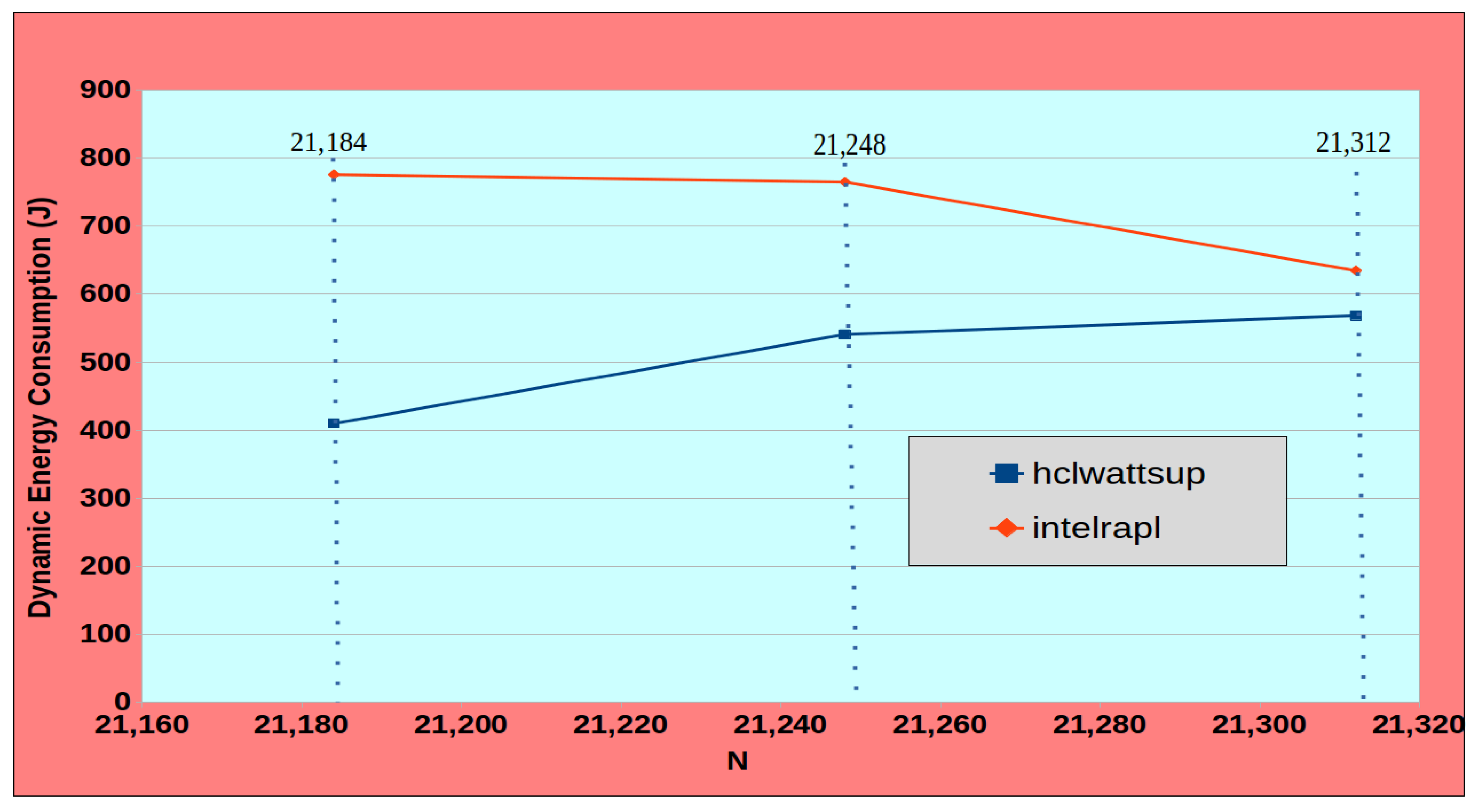
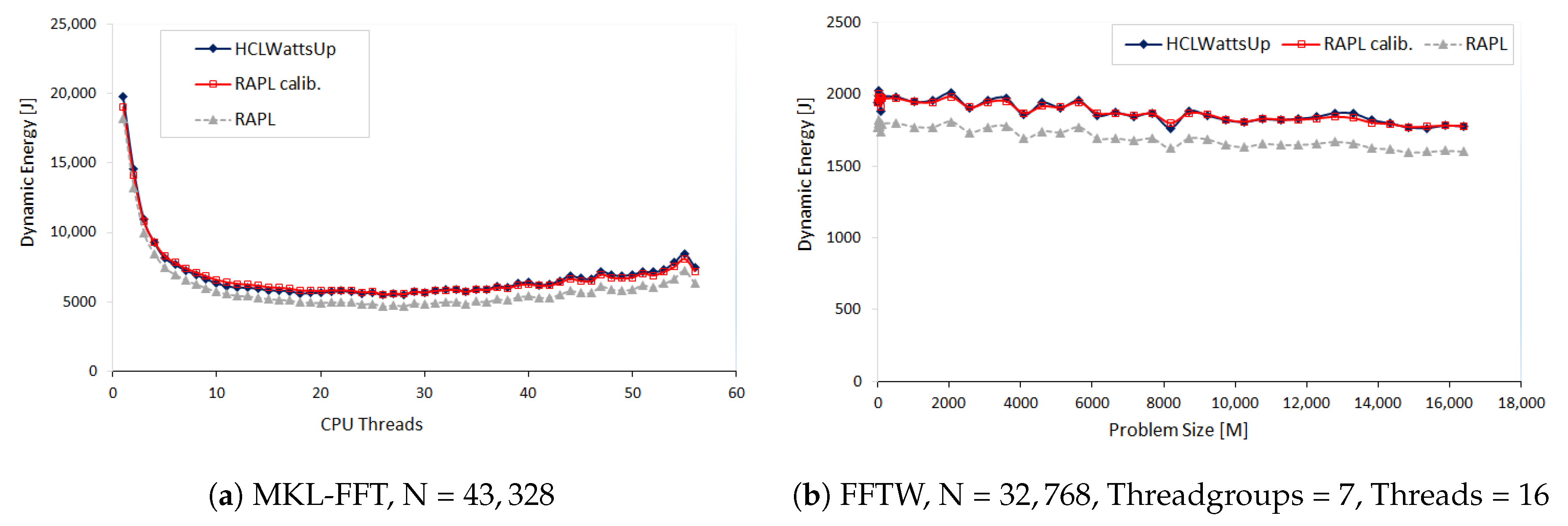
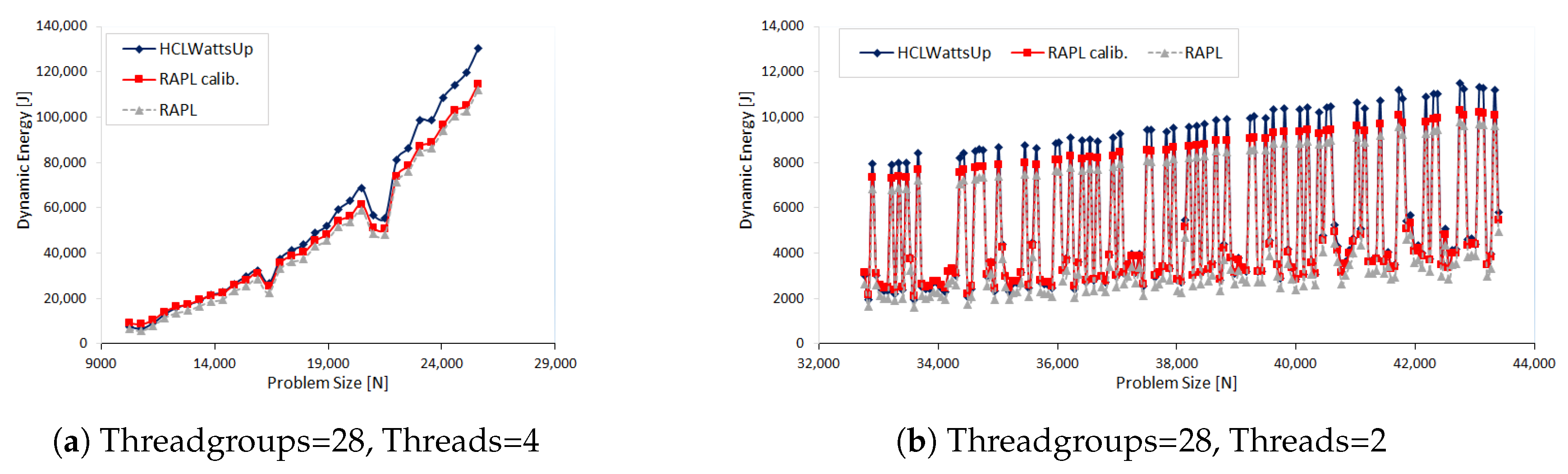
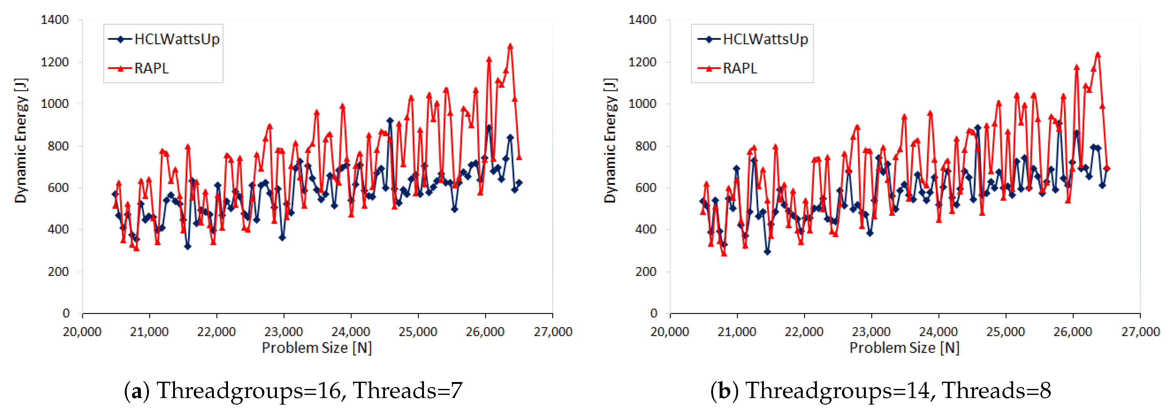
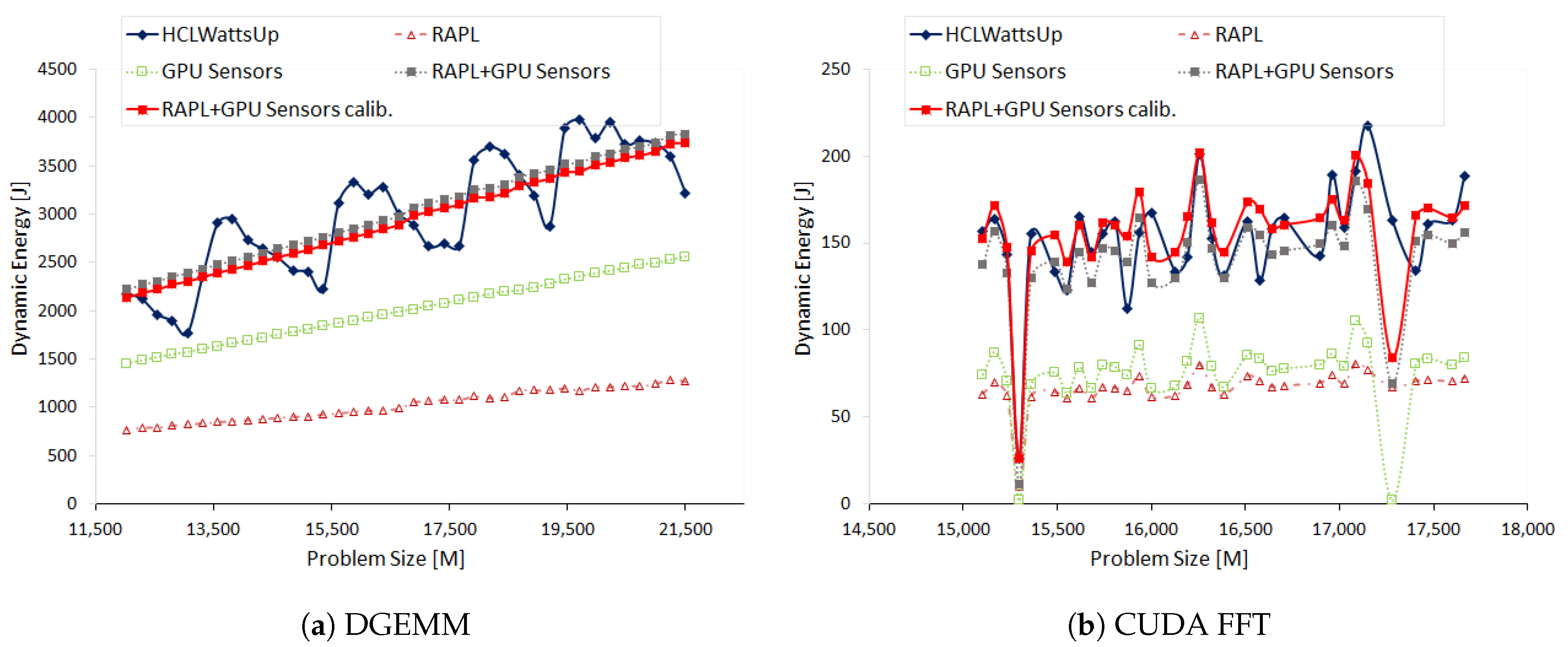
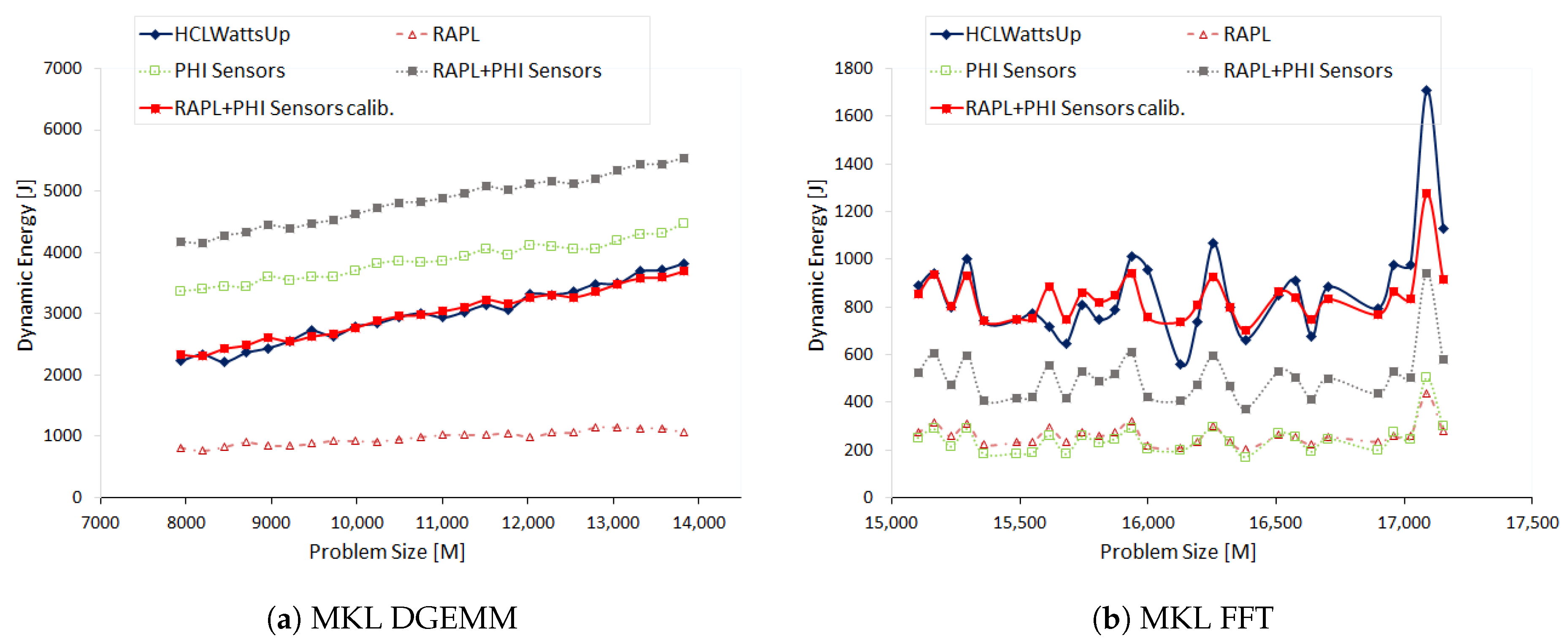
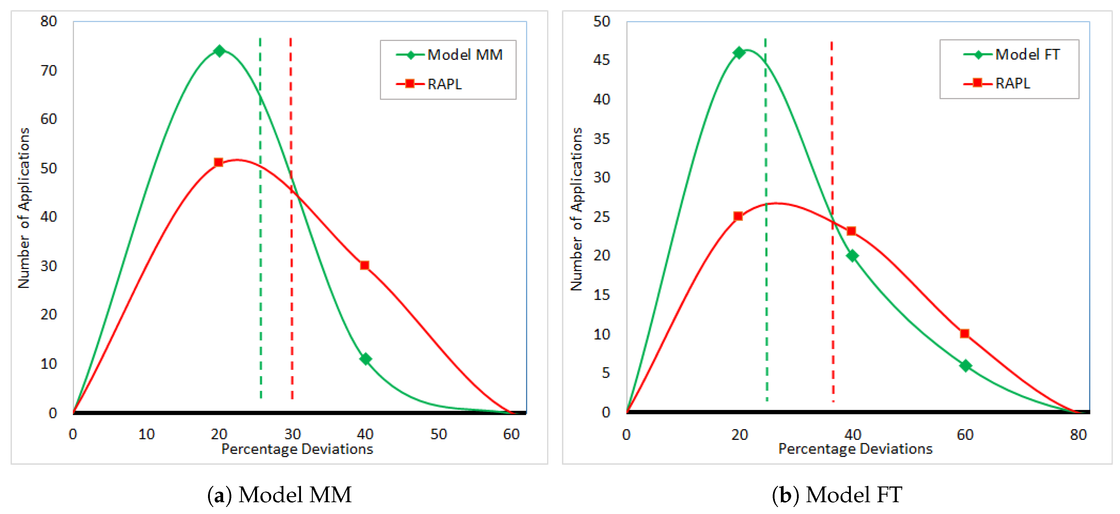
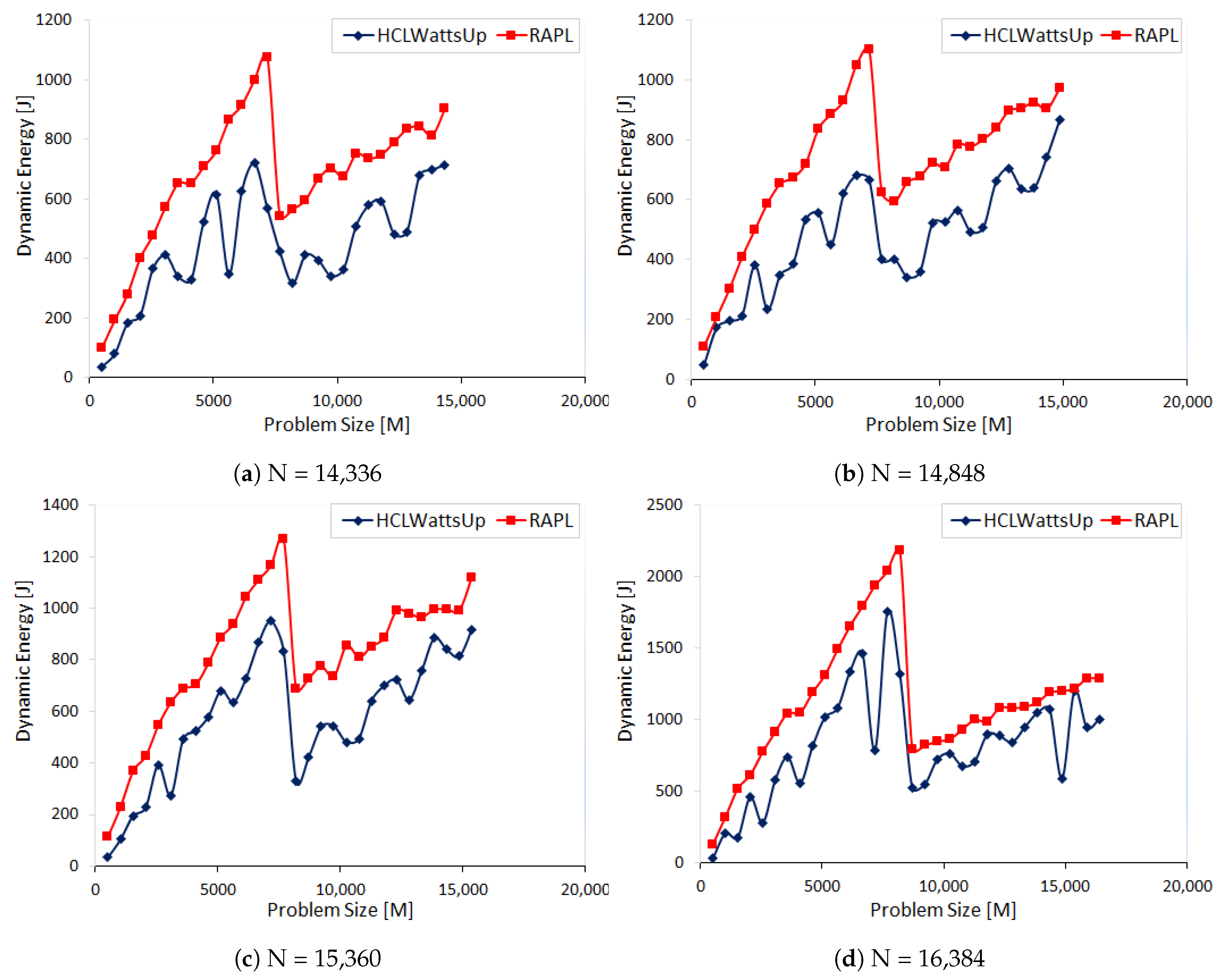
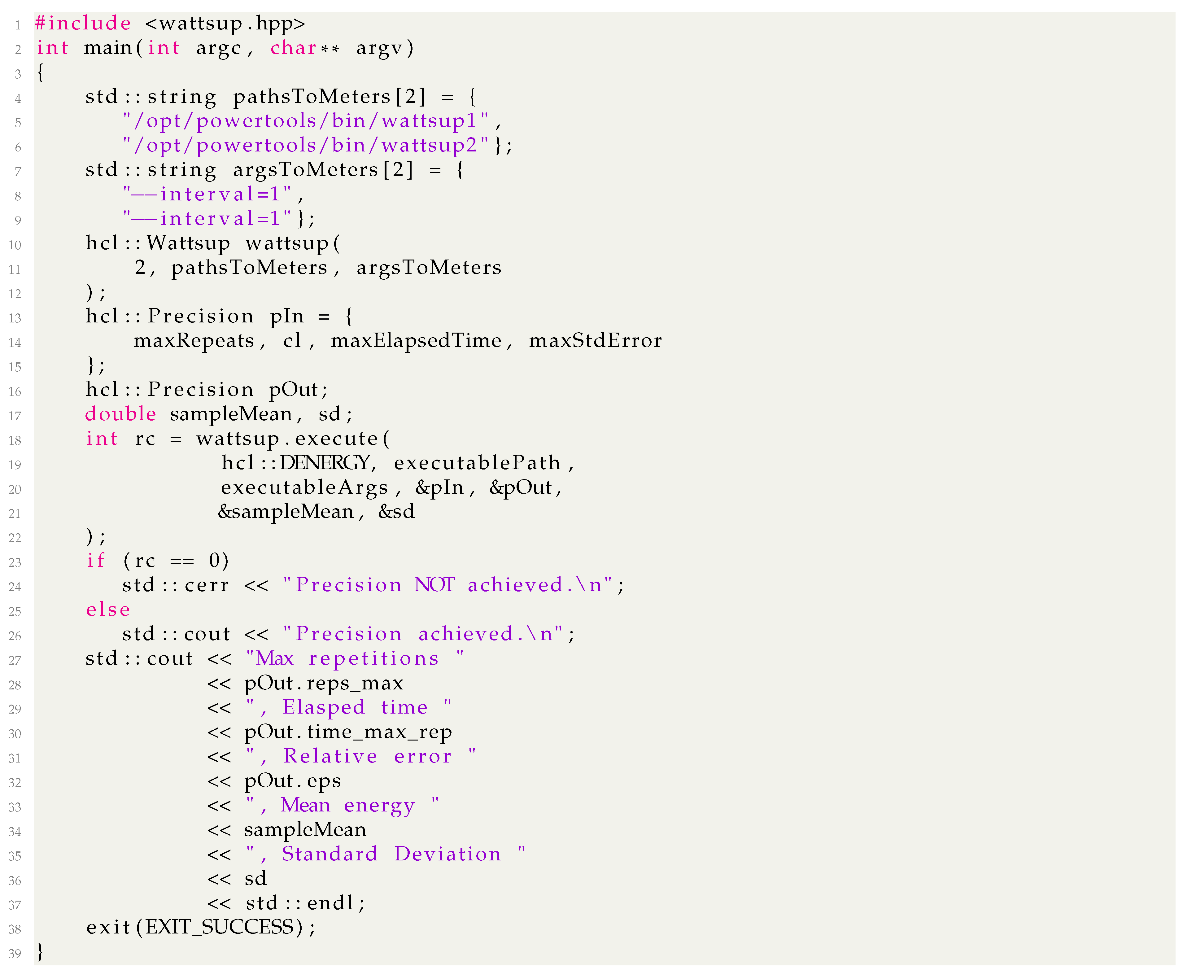
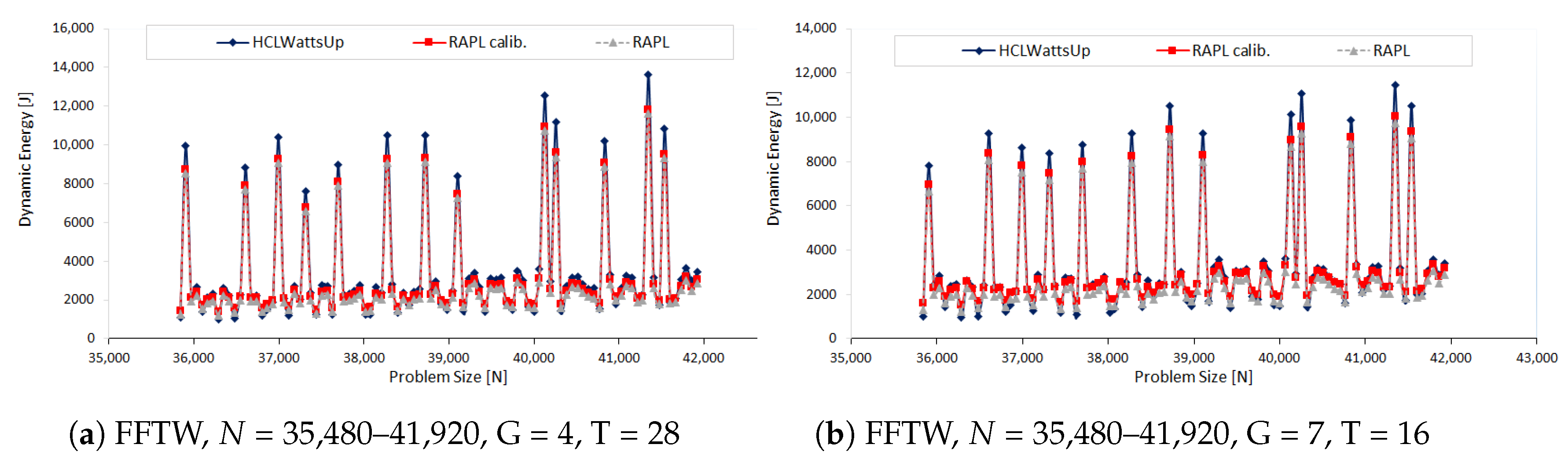
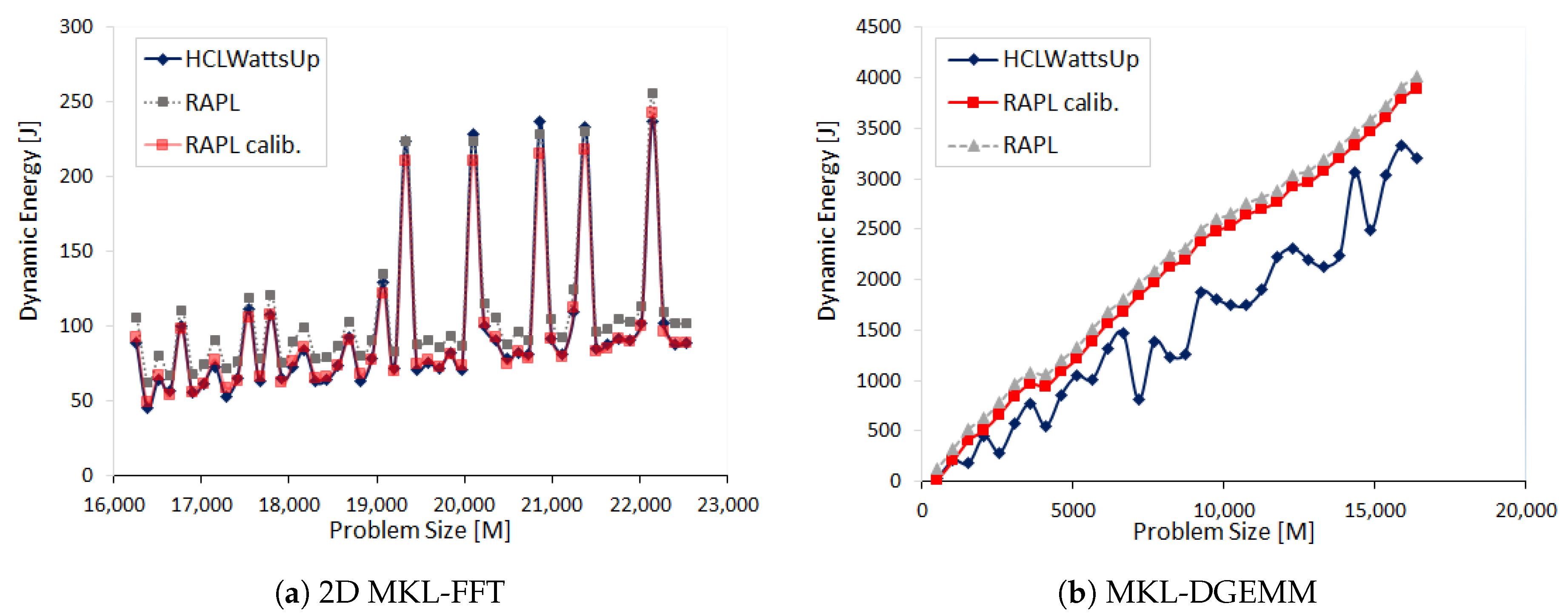
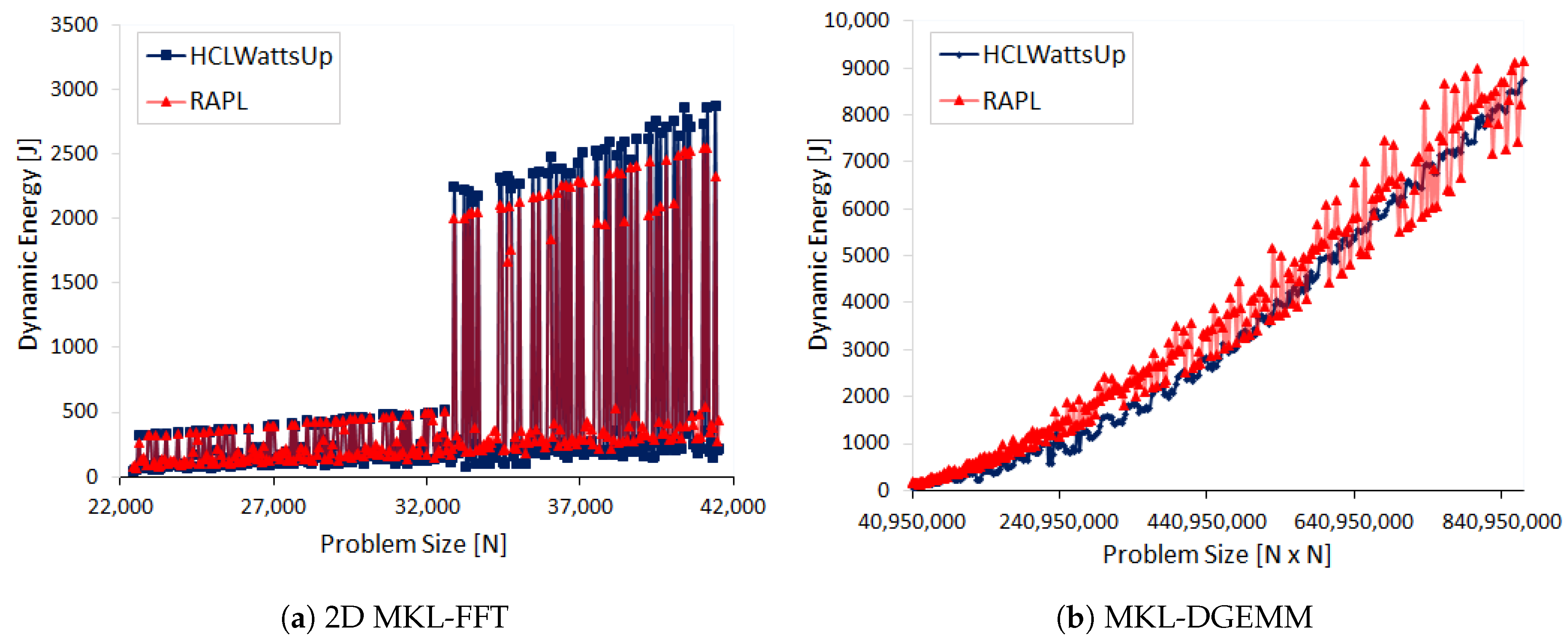
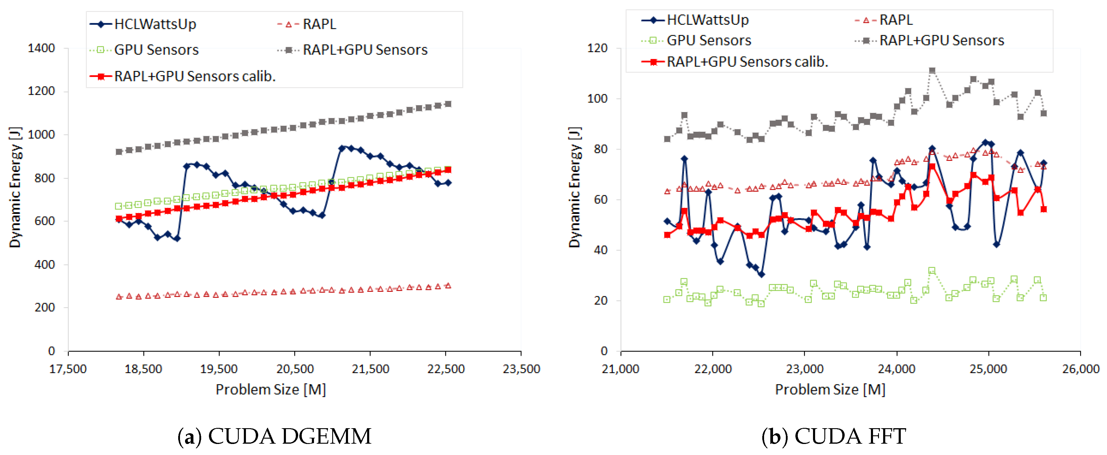
Table A1.
Percentage error of dynamic energy consumption with RAPL and HCLWattsUp on HCLServer03. G = Threadgroups and T = Threads.
Table A1.
Percentage error of dynamic energy consumption with RAPL and HCLWattsUp on HCLServer03. G = Threadgroups and T = Threads.
| Application | Problem Size, Step-Size | Configuration Parameter | Avg Actual Error | Avg. Error after Calibration | Reduction after Calibration |
|---|---|---|---|---|---|
| FFTW | N = | CPU Threads (1–112) | 12.68% | 3.69% | 70.9% |
| MKL-FFT | N = | CPU Cores (1–56) | 13.05% | 2.19% | 83.22% |
| FFTW | N = 20,480–21560, SS = 512 | problem size () where | 8.15% | 5.56% | 31.78 |
| FFTW | N = , SS = 16 | Load Imbalance: problem size () where | 10.45% | 0.6% | 94.26% |
Table A2.
Percentage error of dynamic energy consumption with RAPL and HCLWattsUp on HCLServer03. G = Threadgroups and T = Threads.
Table A2.
Percentage error of dynamic energy consumption with RAPL and HCLWattsUp on HCLServer03. G = Threadgroups and T = Threads.
| Application | Problem Size, Step-Size | Configuration Parameter | Avg Actual Error | Avg. Error after Calibration | Reduction after Calibration |
|---|---|---|---|---|---|
| OpenBlas DGEMM | N = 10,240–25,600, SS = 512 | CPU Threads | |||
| G = 56, T = 2 | 12.84% | 6.66% | 48.13% | ||
| G = 28, T = 4 | 13.28% | 8.58% | 35.39% | ||
| G = 16, T = 7 | 14.02% | 8.54% | 39.09% | ||
| G = 14, T = 8 | 13.61% | 7.98% | 41.37% | ||
| G = 8, T = 14 | 18.59% | 9.64% | 48.14% | ||
| G = 7, T = 16 | 19% | 9.7% | 48.95% | ||
| G = 4, T = 28 | 20.89% | 10.38% | 50.31% | ||
| G = 2, T = 56 | 23.41% | 11.21% | 52.11% | ||
| MKL-FFT | N = 32,768–43,456, SS = 64 | problem size | |||
| G = 28, T = 2 | 15.08% | 4.91% | 67.4% | ||
| G = 14, T = 4 | 13.63% | 4.97% | 63.54% | ||
| G = 8, T = 7 | 13.24% | 5.25% | 60.35 | ||
| G = 7, T = 8 | 13.21% | 5.4% | 59.12% | ||
| G = 4, T = 14 | 13.03% | 5.65% | 56.64% | ||
| G = 2, T = 28 | 13.02% | 5.64% | 56.68% | ||
| G = 1, T = 56 | 14.12% | 6.22% | 55.95% | ||
| MKL-FFT | N = 25,600–46,080, SS = 512 | problem size | |||
| G = 28, T = 2 | 14.46% | 5% | 65.42% | ||
| G = 14, T = 4 | 13% | 4.51% | 65.31% | ||
| G = 8, T = 7 | 12.4% | 4.49% | 63.79% | ||
| G = 7, T = 8 | 12.34% | 4.45% | 63.94% | ||
| G = 4, T = 14 | 11.97% | 4.58% | 61.74% | ||
| G = 2, T = 28 | 12.35% | 4.8% | 61.13% | ||
| G = 1, T = 56 | 13.56% | 6.27% | 53.76% | ||
| FFTW | N = 35,480–41,920, SS = 64 | problem size | |||
| G = 16, T = 7 | 12.4% | 10.35% | 16.53% | ||
| G = 14, T = 8 | 13.19% | 11.54% | 12.51% | ||
| G = 8, T = 14 | 13.66% | 12.73% | 6.81%% | ||
| G = 7, T = 16 | 14.59% | 13.3% | 8.84% | ||
| G = 4, T = 28 | 13.73% | 12.78% | 6.92% | ||
| G = 2, T = 56 | 12.3% | 5.58% | 54.63% | ||
| G = 1, T = 112 | 24.62% | 3.9% | 84.16% |
Table A3.
Percentage error of dynamic energy consumption with RAPL and HCLWattsUp on HCLServer03. ’-’ denotes that calibration does not be improve the difference.
Table A3.
Percentage error of dynamic energy consumption with RAPL and HCLWattsUp on HCLServer03. ’-’ denotes that calibration does not be improve the difference.
| Application | Problem Size, Step-Size | Configuration Parameter | Avg Actual Error | Avg. Error after Calibration | Reduction after Calibration |
|---|---|---|---|---|---|
| FFTW | N = 30,720–34,816, SS = 64 | problem size | |||
| G = 16, T = 7 | 14.51% | - | - | ||
| G = 14, T = 8 | 16.32% | - | - | ||
| G = 8, T = 14 | 16.15% | - | - | ||
| G = 7, T = 16 | 14.89% | - | - | ||
| G = 4, T = 28 | 9.32% | - | - | ||
| G = 2, T = 56 | 10.94% | 5.34% | 51.19% | ||
| G = 1, T = 112 | 25.05% | 10.44% | 58.32% | ||
| FFTW | N = 20,480–26,560, SS = 64 | problem size | |||
| G = 16, T = 7 | 31% | - | - | ||
| G = 14, T = 8 | 28.16% | - | - | ||
| G = 8, T = 14 | 21.59% | - | - | ||
| G = 7, T = 16 | 17.76% | - | - | ||
| G = 4, T = 28 | 7.6% | 4.83 | 36.45% | ||
| G = 2, T = 56 | 9.76% | 6.12% | 37.3% | ||
| G = 1, T = 112 | 25.63% | 10.22% | 60.12 |
Appendix F. Experimental Results of RAPL and HCLWattsUp on HCLServer01 and HCLServer02
For our sets of experiments on HCLServer01 and HCLServer02, we use fixed number of cores and build the application profile as a function of problem size. On HCLServer01, the workload sizes for MKL-DGEMM range from 512 × 16,384 to 16,384 × 16,384 with a step size of 512 and for 2D MKL-FFT range from 16256 × 22,528 to 22,528 × 22,528 with a step size of 128. On HCLServer02, the workload sizes for MKL-DGEMM range from 6400 × 6400 to 29,504 × 29,504 with a step size of 64. For 2D-FFT executed on HCLServer02, the workload sizes range from 22,400 × 22,400 to 41,536 × 41,536 with a step size of 64.
Figure A3a,b show the dynamic energy profiles of 2D MKL-FFT and MKL-DGEMM on HCLServer01 respectively. For most of the data points in dynamic energy profile of 2D MKL-FFT, RAPL reports more dynamic energy consumption than HCLWattsUp. There are, however, many data points where it reports otherwise. The maximum and average errors of RAPL with HCLWattsUp is 37.1% and 16.01%. We can reduce them to 9.93% and 3.48% by calibrating RAPL readings.
Figure A3.
Dynamic energy consumption of RAPL, RAPL calibrated and HCLWattsUp on HCLServer01.

Figure A4.
Dynamic energy consumption of RAPL and HCLWattsUp on HCLServer02.

For MKL-DGEMM on HCLServer01, we find that RAPL readings are leading the HCLWattsUp readings. Further, both profiles do not exhibit the same pattern. One can observe many data points such as 1024 × 16,384, 2048 × 16,384, 6656 × 16,384, 14,336 × 16,384 and et cetera, where HCLWattsUp suggests an increase of 14.67%, 81.53%, 55.05%, 23.2% in dynamic energy consumption whereas RAPL suggest a decrease of 38.25%, 8.05%, 19.89%, 3.76%. The maximum and average difference of RAPL with HCLWattsUp is 266.42% and 62.42%. However, we can reduce this error to 130.53% and 42.87% using calibrating RAPL readings. But, this increases the divergence between the data points where both the tools provide dynamic energy consumption values oppositely. Consider, for example, the data point 1024 × 16,384. RAPL, after calibrating, suggests a decrease of 49.12% which was 38.25% in the absence of calibration.
Figure A4a,b show the dynamic energy profiles of 2D MKL-FFT and MKL-DGEMM on HCLServer02 respectively. For most of the data points of MKL-DGEMM profile, RAPL suggests a decrease in dynamic energy consumption whereas HCLWattsUp reports the otherwise and vice versa. Consider, for example, the problem sizes 43454464, 125440000, 228130816, 270536704 and others where RAPL suggests a decrease of 11.92%, 15.29%, 8.68%, 27.6% whereas HCLWattsUp suggests an increase of 41.11%, 30.59%, 70.24%, 37.94%; and the problem sizes, for example, 42614784, 170459136, 249892864, 268435456 and others where RAPL suggests an increase of 14.09%, 17.3%, 20.92%, 38.99% whereas HCLWattsUp suggests a decrease of 29.67%, 19.51%, 11.83%, 28.75%. The maximum and average difference between both profiles is 205% and 36.13%.
We also find many such data points in MKL-FFT profile where both the tools reports the dynamic energy consumption oppositely. Consider, for example, the problem sizes 916393984, 1167998976, 1425817600, 1450086400 where RAPL suggests a decrease of 12.39%, 31.33%, 18.77%, 5.4% whereas HCLWattsUp reports an increase of 11.68%, 35.84%, 6.46%, 31.25%; and the the problem sizes such as 507510784, 800210944, 1150566400, 1099055104 and others where RAPL suggests an increase of 1.26%, 19.9%, 40.87%, 4.74% whereas HCLWattsUp suggests a decrease of 22.24%, 4.79%, 9.54%, 6.02%, 28.75%. The maximum and average difference between both profiles is 156.38% and 28.67%.
Table A4 presents the prediction errors of RAPL against HCLWattsUp on HCLServer01 and HCLServer02. We also present the percentage of error reduction between the dynamic energy profiles with RAPL and power meter after using calibration.
Table A4.
Percentage error of dynamic energy consumption with RAPL and HCLWattsUp on HCLServer01 and HCLServer02. ’-’ denotes that calibration does not improve the difference.
Table A4.
Percentage error of dynamic energy consumption with RAPL and HCLWattsUp on HCLServer01 and HCLServer02. ’-’ denotes that calibration does not improve the difference.
| Application | Platform | Avg | Max | Min | Avg after Calibration | Reduction after Calibration |
|---|---|---|---|---|---|---|
| FFT | HCLServer01 | 16.01% | 37.1% | 0.01% | 3.48% | 78.26% |
| DGEMM | HCLServer01 | 62.42% | 266.42% | 12.54% | 42.86% | 31.34% |
| FFT | HCLServer02 | 28.67% | 156.38% | 0.03% | - | - |
| DGEMM | HCLServer02 | 36.13% | 205% | 0.39% | - | - |
Appendix G. Methodology To Compare Measurements Using Sensors and HCLWattsUp
To analyze the dynamic energy consumption by a given component when running an application, we need to build application profiles on them. HCLWattsUp API provides the dynamic energy consumption of application instead of component. It, therefore, contains the contributions by other components including CPU host-core and DRAM. Built-in sensors, on the other hand, only provide the power consumption of GPU or Xeon Phi only (we offload the applications to run on Intel Xeon Phi, so it includes the CPU host core, DRAM and PCIe to copy and migrate the data between CPU host core and Xeon Phi) Therefore, to compare both methodologies in a most fair equitable way and to obtain the dynamic energy profiles of applications, we use RAPL as an aide to sensors for determining the application energy. Because, RAPL also determine the power consumption of CPU and DRAM using on-chip voltage regulator and current sensor [8].
Now, we present the work-flow of experiments that we follow to determine the dynamic energy consumption of the application. To obtain the CPU host-core and DRAM contribution in dynamic energy consumption of the application, we use RAPL in following way:
- Using Intel PCM/PAPI, we obtain the base power of CPU and DRAM (when the given application is not running).
- Using HCLWattsUp API, we obtain the execution time of the given application.
- Using Intel PCM/PAPI, we obtain the total energy consumption of the CPU host-core (because all other cores are idle) and DRAM, during the execution of the given application.
- Finally, we calculate the dynamic energy consumption (of CPU and DRAM) by subtracting the base energy from total energy consumed during the execution of the given application.
To obtain the GPU/Xeon Phi contribution, we use NVML/Intel SMC in following way:
- Using NVML/Intel SMC, we obtain the base power of GPU/Xeon Phi (when the given application is not running).
- Using HCLWattsUp API, we obtain the execution time of the given application.
- Using NVML/Intel SMC, we obtain the total energy consumption of GPU/Xeon Phi during the execution of the given application.
- Finally, we calculate the dynamic energy consumption GPU/Xeon Phi by subtracting the base energy from total energy consumed during the execution of the given application.
Now, we present the workflow of the experiments to determine the dynamic energy consumption by the given application kernel, using HCLWattsUp:
- Using HCLWattsUp API, we obtain the base power of the server (when the given application is not running).
- Using HCLWattsUp API, we obtain the execution time of the application.
- Using HCLWattsUp API, we obtain the total energy consumption of the server, during the execution of the given application.
- Finally, we calculate the dynamic energy consumption by subtracting the base power from total energy consumed during the execution of the given application.
Important to note here, the execution time of the application kernel is the same for dynamic energy calculations by all tools. So, any difference between the energy readings using these tools comes solely from their power readings. The cost in terms of number of measurements to determine a single data point of an application dynamic energy profile using sensors is higher than using HCLWattsUp API. Because we need at least five (Base power with RAPL, Total Energy with RAPL, Base power with NVML/Intel SMC, Total Energy with NVML/Intel SMC, and Execution Time) measurements to obtain the data point of the given application dynamic energy profile using RAPL and GPU/Xeon Phi internal sensors. However, we just need three measurements to obtain it using HCLWattsUp.
Appendix H. Comparison of Measurements by GPU Sensors with HCLWattsUp on HCLServer02
On Nvidia P100 GPU on HCLServer02, we build the dynamic energy profile of 2D FFT as a function of problem size ranging from to with a constant step size of 64, using sensors and HCLWattsUp. Figure A5b illustrates the dynamic energy profiles of 2D FFT using sensors and HCLWattsUp. We find that sensors follow the trend of HCLWattsUp for 57.14% of the data points. Consider, for example, the data points , and where HCLWattsUp suggests an increase of 33.53%, 15.4% and 18.49% whereas sensors suggest an increase of 2.32%, 3.21% and 6.54% respectively. The maximum and average errors are 175.97% and 73.34%. We can reduce them using calibration to 51.24% and 16.95% respectively.
RAPL and GPU sensors follow the same trend for 88.89% of the data points. It reflects that the difference with HCLWattsUp comes from both together. But, the combined profile follows the GPU sensors trend and diverges with HCLWattsUp for 51.11% of the data points. Hence, the difference between (RAPL and GPU) sensors and HCLWattsUp is mainly from GPU sensors because they are driving the combined profile. Consider, for example, the data point . RAPL suggests an increase of 6.42% in dynamic energy consumption with respect to the previous data point. However, GPU sensors suggest a decrease of 38.12% for it and we find a decrease of 2.91% in combined profile of sensors.
We also observe that RAPL reports more dynamic energy than GPU sensors. It means that for this application configuration, data transfer between CPU host-core, DRAM and GPU consumes more dynamic energy than the computation on P100 GPU.
Figure A5.
Dynamic energy consumption profiles of Nvidia P100 PCIe GPU on HCLServer02.

We execute DGEMM on HCLServer02 with workload sizes ranging from 18,176 × 22,528 to 22,528 × 22,528 with a constant step size of 128. Figure A5a illustrates the dynamic energy profiles of DGEMM using HCLWattsUp and sensors (RAPL and GPU sensors) Like K40c GPU on HCLServer01, the combined energy profile of DGEMM with (RAPL and NVML) sensors exhibit a linear profile whereas HCLWattsUp exhibit differently. We find that combined sensors do not follow the application behavior exhibited by HCLWattsUp for 64.71% of the data points. Consider, for example, the data points (): 218,560 × 22,528, 18,944 × 22,528 and 22,400 × 22,528 where HCLWattsUp demonstrate a decrease of 4.14%, 3.8% and 5.32% whereas sensors exhibit an increase of 1.23%, 1.06% and 0.59% respectively. The maximum and average errors are 84.84% and 40.06%. They can be reduced using calibration to 26.07% and 11.62% respectively.
Table A5.
Percentage error of dynamic energy consumption by Nvidia P100 PCIe GPU with and without calibration and HCLWattsUp on HCLServer02.
Table A5.
Percentage error of dynamic energy consumption by Nvidia P100 PCIe GPU with and without calibration and HCLWattsUp on HCLServer02.
| Without Calibration | |||
|---|---|---|---|
| Application | Min | Max | Avg |
| DGEMM | 13.11% | 84.84% | 40.06% |
| FFT | 17.91% | 175.97% | 73.34% |
| With Calibration | |||
| Application | Min | Max | Avg |
| DGEMM | 0.07% | 26.07% | 11.62% |
| FFT | 0.025% | 51.24% | 16.95% |
Appendix I. Costs of Measurement of the Three Approaches
In this section, we compare the cost in terms of number of measurements to determine a single data point of an application dynamic energy profile with aforementioned tools. To determine the dynamic energy consumption by a given workload size of an application, we need following three measurements with RAPL and HCLWattsUp:
- Base power
- Execution time of the application
- Total Energy consumed by the application during the execution
However, the cost of determining the dynamic energy consumption with (RAPL and on-chip GPU/Xeon Phi) sensors is comparatively higher, because we need at least following five measurements:
- Base power with RAPL
- Total Energy with RAPL
- Base power with NVML/Intel SMC
- Total Energy with NVML/Intel SMC
- Execution Time
We need just one measurement to predict the dynamic energy consumption with PMC based energy predictive models but the cost of building the model is relatively higher. In order to build a model (either platform-level or application specific), one needs to collect a huge data set containing all the PMCs of a given application on a platform with its dynamic energy consumption. For example, on Intel Haswell EP multicore CPU on HCLServer01 (see Table 1), collecting all the PMCs for an application using Likwid tool takes at minimum 53 times of its execution. Furthermore, after collection of PMCs, selecting suitable PMCs for producing accurate energy models is also a tedious job.
Appendix J. Benchmark Suite for Comparison of Dynamic Energy Consumption using PMC-Based Energy Predictive Models and HCLWattsUp
Table A6.
List of Applications.
| Application | Description |
|---|---|
| MKL FFT | Fast Fourier Transform |
| MKL DGEMM | Dense Matrix Multiplication |
| HPCG | High performance conjugate gradient |
| NPB IS | Integer Sort, Kernel for random memory access |
| NPB LU | Lower-Upper Gauss-Seidel solver |
| NPB EP | Embarrassingly Parallel, Kernel |
| NPB BT | Block Tri-diagonal solver |
| NPB MG | Multi-Grid on a sequence of meshes |
| NPB FT | Discrete 3D fast Fourier Transform |
| NPB DC | Data Cube |
| NPB UA | Unstructured Adaptive mesh, dynamic memory access |
| NPB CG | Conjugate Gradient |
| NPB SP | Scalar Penta-diagonal solver |
| NPB DT | Data traffic |
| stress | CPU, disk and I/O stress |
| Naive MM | Naive Matrix-matrix multiplication |
| Naive MV | Naive Matrix-vector multiplication |
References
- IEA. International Energy Agency (IEA) at COP21; IEA: Paris, France, 2015. [Google Scholar]
- Jones, N. How to stop data centres from gobbling up the world’s electricity. Nature 2018, 561, 163–166. [Google Scholar] [CrossRef] [PubMed]
- ATAG. Air Transport Action Group (ATAG): Facts and Figures; ATAG: Dunfermline, UK, 2018. [Google Scholar]
- Andrae, A.; Edler, T. On Global Electricity Usage of Communication Technology: Trends to 2030. Challenges 2015, 6, 117–157. [Google Scholar] [CrossRef]
- Konstantakos, V.; Chatzigeorgiou, A.; Nikolaidis, S.; Laopoulos, T. Energy Consumption Estimation in Embedded Systems. IEEE Trans. Instrum. Meas. 2008, 57, 797–804. [Google Scholar] [CrossRef] [Green Version]
- Rotem, E.; Naveh, A.; Ananthakrishnan, A.; Weissmann, E.; Rajwan, D. Power-Management Architecture of the Intel Microarchitecture Code-Named Sandy Bridge. IEEE Micro 2012, 32, 20–27. [Google Scholar] [CrossRef]
- David, H.; Gorbatov, E.; Hanebutte, U.R.; Khanna, R.; Le, C. RAPL: Memory power estimation and capping. In Proceedings of the 2010 ACM/IEEE International Symposium on Low-Power Electronics and Design (ISLPED), Austin, TX, USA, 18–20 August 2010; pp. 189–194. [Google Scholar]
- Gough, C.; Steiner, I.; Saunders, W. ; Energy Efficient Servers: Blueprints for Data Center Optimization; Apress: New York, NY, USA, 2015; ISBN 978-1-4302-6638-9. [Google Scholar]
- Intel Corporation. Intel® Xeon Phi™ Coprocessor System Software Developers Guide; Intel Corporation: Santa Clara, CA, USA, 2014. [Google Scholar]
- Intel Corporation. Intel® Manycore Platform Software Stack (Intel MPSS); Intel Corporation: Santa Clara, CA, USA, 2014. [Google Scholar]
- Advanced Micro Devices. BIOS and Kernel Developer’s Guide (BKDG) for AMD Family 15h Models 00h-0Fh Processors; Advanced Micro Devices: Santa Clara, CA, USA, 2012. [Google Scholar]
- Hackenberg, D.; Ilsche, T.; Schöne, R.; Molka, D.; Schmidt, M.; Nagel, W.E. Power measurement techniques on standard compute nodes: A quantitative comparison. In Proceedings of the 2013 IEEE International Symposium on Performance Analysis of Systems and Software (ISPASS), Austin, TX, USA, 21–23 April 2013; IEEE: Piscataway, NJ, USA, 2013; pp. 194–204. [Google Scholar]
- Nvidia. Nvidia Management Library: NVML Reference Manual; Nvidia: Santa Clara, CA, USA, 2018. [Google Scholar]
- Burtscher, M.; Zecena, I.; Zong, Z. Measuring GPU Power with the K20 Built-in Sensor. In Proceedings of the Workshop on General Purpose Processing Using GPUs, GPGPU-7, Salt Lake City, UT, USA, 1 March 2014; ACM: New York, NY, USA, 2014; pp. 28:28–28:36. [Google Scholar]
- Economou, D.; Rivoire, S.; Kozyrakis, C.; Ranganathan, P. Full-system power analysis and modeling for server environments. In International Symposium on Computer Architecture; IEEE: Piscataway, NJ, USA, 2006; pp. 70–77. [Google Scholar]
- McCullough, J.C.; Agarwal, Y.; Chandrashekar, J.; Kuppuswamy, S.; Snoeren, A.C.; Gupta, R.K. Evaluating the Effectiveness of Model-based Power Characterization. In Proceedings of the 2011 USENIX Conference on USENIX Annual Technical Conference (USENIXATC’11), USENIX Association, Oregon, Portland, 15–17 June 2011; p. 12. [Google Scholar]
- O’brien, K.; Pietri, I.; Reddy, R.; Lastovetsky, A.; Sakellariou, R. A Survey of Power and Energy Predictive Models in HPC Systems and Applications. Acm Comput. Surv. 2017, 50, 37:1–37:38. [Google Scholar] [CrossRef]
- Shahid, A.; Fahad, M.; Reddy, R.; Lastovetsky, A. Additivity: A Selection Criterion for Performance Events for Reliable Energy Predictive Modeling. Supercomput. Front. Innov. Int. J. 2017, 4, 50–65. [Google Scholar]
- Heterogeneous Computing Laboratory. HCLWattsUp: Software API for Power and Energy Measurements Using WattsUp Pro Meter; School of Computer Science, University College Dublin: Dublin, Ireland, 2019. [Google Scholar]
- Hackenberg, D.; Schöne, R.; Ilsche, T.; Molka, D.; Schuchart, J.; Geyer, R. An Energy Efficiency Feature Survey of the Intel Haswell Processor. In Proceedings of the 2015 IEEE International Parallel and Distributed Processing Symposium Workshop, Hyderabad, India, 25—29 May 2015; pp. 896–904. [Google Scholar]
- Bellosa, F. The Benefits of Event: Driven Energy Accounting in Power-sensitive Systems. In Proceedings of the 9th Workshop on ACM SIGOPS European Workshop: Beyond the PC: New Challenges for the Operating System (EW 9), Kolding, Denmark, 17–20 September 2000; ACM: New York, NY, USA, 2000; pp. 37–42. [Google Scholar]
- Isci, C.; Martonosi, M. Runtime power monitoring in high-end processors: Methodology and empirical data. In Proceedings of the 36th Annual IEEE/ACM International Symposium on Microarchitecture, MICRO-36, San Diego, CA, USA, 5 December 2003; IEEE: Washington, DC, USA, 2003; pp. 93–104. [Google Scholar]
- Li, T.; John, L.K. Run-time Modeling and Estimation of Operating System Power Consumption. Sigmetrics Perform. Eval. Rev. 2003, 31, 160–171. [Google Scholar] [CrossRef]
- Lee, B.C.; Brooks, D.M. Accurate and Efficient Regression Modeling for Microarchitectural Performance and Power Prediction. Sigarch Comput. Archit. News 2006, 34, 185–194. [Google Scholar] [CrossRef]
- Heath, T.; Diniz, B.; Carrera, E.V.; Meira, W., Jr.; Bianchini, R. Energy Conservation in Heterogeneous Server Clusters. In Proceedings of the Tenth ACM SIGPLAN Symposium on Principles and Practice of Parallel Programming (PPoPP ’05), Chicago, IL, USA, 15–17 June 2005; ACM: New York, NY, USA, 2005; pp. 186–195. [Google Scholar]
- Fan, X.; Weber, W.D.; Barroso, L.A. Power Provisioning for a Warehouse-sized Computer. In Proceedings of the 34th Annual International Symposium on Computer Architecture (ISCA ’07), San Diego, CA, USA, 9–13 June 2017; ACM: New York, NY, USA, 2007; pp. 13–23. [Google Scholar]
- Singh, K.; Bhadauria, M.; McKee, S.A. Real Time Power Estimation and Thread Scheduling via Performance Counters. Sigarch Comput. Archit. News 2009, 37, 46–55. [Google Scholar] [CrossRef]
- Goel, B.; McKee, S.A.; Gioiosa, R.; Singh, K.; Bhadauria, M.; Cesati, M. Portable, scalable, per-core power estimation for intelligent resource management. In Proceedings of the International Conference on Green Computing, Chicago, IL, USA, 15–18 August 2010; pp. 135–146. [Google Scholar]
- Basmadjian, R.; Ali, N.; Niedermeier, F.; de Meer, H.; Giuliani, G. A Methodology to Predict the Power Consumption of Servers in Data Centres. In Proceedings of the 2nd International Conference on Energy-Efficient Computing and Networking (e-Energy ’11), New York, NY, USA, 31 May–1 June 2011; ACM: New York, NY, USA, 2011; pp. 1–10. [Google Scholar]
- Bircher, W.L.; John, L.K. Complete System Power Estimation Using Processor Performance Events. IEEE Trans. Comput. 2012, 61, 563–577. [Google Scholar] [CrossRef]
- Dargie, W. A Stochastic Model for Estimating the Power Consumption of a Processor. IEEE Trans. Comput. 2015, 64, 1311–1322. [Google Scholar] [CrossRef]
- Lastovetsky, A.; Reddy, R. New Model-Based Methods and Algorithms for Performance and Energy Optimization of Data Parallel Applications on Homogeneous Multicore Clusters. IEEE Trans. Parallel Distrib. Syst. 2017, 28, 1119–1133. [Google Scholar] [CrossRef]
- Li, S.; Ahn, J.H.; Strong, R.D.; Brockman, J.B.; Tullsen, D.M.; Jouppi, N.P. The McPAT Framework for Multicore and Manycore Architectures: Simultaneously Modeling Power, Area, and Timing. ACM Trans. Archit. Code Optim. 2013, 10, 5. [Google Scholar] [CrossRef]
- Haj-Yihia, J.; Yasin, A.; Asher, Y.B.; Mendelson, A. Fine-grain power breakdown of modern out-of-order cores and its implications on Skylake-based systems. ACM Trans. Archit. Code Optim. (TACO) 2016, 13, 56. [Google Scholar] [CrossRef]
- Mair, J.; Huang, Z.; Eyers, D. Manila: Using a densely populated pmc-space for power modelling within large-scale systems. Parallel Comput. 2019, 82, 37–56. [Google Scholar] [CrossRef]
- Hong, S.; Kim, H. An Integrated GPU Power and Performance Model. Sigarch Comput. Archit. News 2010, 38, 280–289. [Google Scholar]
- Nagasaka, H.; Maruyama, N.; Nukada, A.; Endo, T.; Matsuoka, S. Statistical power modeling of GPU kernels using performance counters. In Proceedings of the International Conference on Green Computing, Chicago, IL, USA, 15–18 August 2010; pp. 115–122. [Google Scholar]
- Song, S.; Su, C.; Rountree, B.; Cameron, K.W. A Simplified and Accurate Model of Power-Performance Efficiency on Emergent GPU Architectures. In Proceedings of the 2013 IEEE 27th International Symposium on Parallel and Distributed Processing, Boston, MA, USA, 20–24 May 2013; pp. 673–686. [Google Scholar]
- Shao, Y.S.; Brooks, D. Energy characterization and instruction-level energy model of Intel’s Xeon Phi processor. In Proceedings of the International Symposium on Low Power Electronics and Design (ISLPED), Beijing, China, 4–6 September 2013; pp. 389–394. [Google Scholar]
- Al-Khatib, Z.; Abdi, S. Operand-Value-Based Modeling of Dynamic Energy Consumption of Soft Processors in FPGA. In Applied Reconfigurable Computing; Sano, K., Soudris, D., Hübner, M., Diniz, P.C., Eds.; Springer International Publishing: Berlin, Germany, 2015; pp. 65–76. [Google Scholar]
- Asanovic, K.; Bodik, R.; Catanzaro, B.C.; Gebis, J.J.; Husbands, P.; Keutzer, K.; Patterson, D.A.; Plishker, W.L.; Shalf, J.; Williams, S.W.; et al. The Landscape of Parallel Computing Research: A View from Berkeley; Technical Report UCB/EECS-2006-183; University of California: Berkeley, CA, USA, 2006. [Google Scholar]
- IntelPCM. Intel® Performance Counter Monitor—A Better Way to Measure CPU Utilization. 2017. Available online: https://software.intel.com/en-us/articles/intel-performance-counter-monitor (accessed on 10 June 2019).
- PAPI. Performance Application Programming Interface 5.4.1. 2015. Available online: https://icl.utk.edu/papi/overview/index.html (accessed on 10 June 2019).
- Manumachu, R.R.; Lastovetsky, A. Bi-Objective Optimization of Data-Parallel Applications on Homogeneous Multicore Clusters for Performance and Energy. IEEE Trans. Comput. 2018, 67, 160–177. [Google Scholar] [CrossRef]
- Reddy Manumachu, R.; Lastovetsky, A.L. Design of self-adaptable data parallel applications on multicore clusters automatically optimized for performance and energy through load distribution. Concurr. Comput. Pract. Exp. 2019, 31, e4958. [Google Scholar] [CrossRef]
- Khaleghzadeh, H.; Zhong, Z.; Reddy, R.; Lastovetsky, A. Out-of-core implementation for accelerator kernels on heterogeneous clouds. J. Supercomput. 2018, 74, 551–568. [Google Scholar] [CrossRef]
- Treibig, J.; Hager, G.; Wellein, G. LIKWID: A Lightweight Performance-Oriented Tool Suite for x86 Multicore Environments. In Proceedings of the 2010 39th International Conference on Parallel Processing Workshops, San Diego, CA, USA, 13–16 September 2010; IEEE: Piscataway, NJ, USA, 2010; pp. 207–216. [Google Scholar] [Green Version]
- Perf Wiki. perf: Linux Profiling with Performance Counters; Wikipedia, the Free Encyclopedia, 2017. Available online: https://perf.wiki.kernel.org/index.php/Main_Page (accessed on 10 June 2019).
- Alonso, P.; Badia, R.M.; Labarta, J.; Barreda, M.; Dolz, M.F.; Mayo, R.; Quintana-Ortí, E.S.; Reyes, R. Tools for Power-Energy Modelling and Analysis of Parallel Scientific Applications. In Proceedings of the 2012 41st International Conference on Parallel Processing, Pittsburgh, PA, USA, 10–13 September 2012; pp. 420–429. [Google Scholar]
- Mantovani, F.; Calore, E. Performance and power analysis of HPC workloads on heterogeneous multi-node clusters. J. Low Power Electron. Appl. 2018, 8, 13. [Google Scholar] [CrossRef]
- Zhou, Z.; Abawajy, J.H.; Li, F.; Hu, Z.; Chowdhury, M.U.; Alelaiwi, A.; Li, K. Fine-Grained Energy Consumption Model of Servers Based on Task Characteristics in Cloud Data Center. IEEE Access 2018, 6, 27080–27090. [Google Scholar] [CrossRef]
- Bedard, D.; Lim, M.Y.; Fowler, R.; Porterfield, A. PowerMon: Fine-grained and integrated power monitoring for commodity computer systems. In Proceedings of the IEEE SoutheastCon 2010 (SoutheastCon), Concord, NC, USA, 18–21 March 2010; pp. 479–484. [Google Scholar]
- Ge, R.; Feng, X.; Song, S.; Chang, H.; Li, D.; Cameron, K.W. PowerPack: Energy Profiling and Analysis of High-Performance Systems and Applications. IEEE Trans. Parallel Distrib. Syst. 2010, 21, 658–671. [Google Scholar] [CrossRef]
- Laros, J.H.; Pokorny, P.; DeBonis, D. PowerInsight—A commodity power measurement capability. In Proceedings of the 2013 International Green Computing Conference Proceedings, Arlington, VA, USA, 27–29 June 2013; pp. 1–6. [Google Scholar]
- Intel Corporation. Intelligent Platform Management Interface Spec; Intel Corporation: Santa Clara, CA, USA, 2013. [Google Scholar]
- Intel Corporation. DCMI—Data Center Manageability Interface Specification; Intel Corporation: Santa Clara, CA, USA, 2011. [Google Scholar]
Figure 1.
Dynamic energy consumption profile segments of HCLWattsUp and Intel RAPL for 2D FFT computation using FFTW-3.3.7 on HCLServer03.
Figure 1.
Dynamic energy consumption profile segments of HCLWattsUp and Intel RAPL for 2D FFT computation using FFTW-3.3.7 on HCLServer03.

Figure 2.
Dynamic energy profiles with Running Average Power Limit (RAPL) and HCLWattsUp on HCLServer03, class A. RAPL calib. means that RAPL readings have been calibrated.
Figure 2.
Dynamic energy profiles with Running Average Power Limit (RAPL) and HCLWattsUp on HCLServer03, class A. RAPL calib. means that RAPL readings have been calibrated.

Figure 3.
Dynamic energy profiles by RAPL and HCLWattsUp on HCLServer03, class B. RAPL calib. means that RAPL readings have been calibrated. (a) DGEMM, N = 10,240–25,600, (b) MKL-FFT, N = 32,768–43,456.
Figure 3.
Dynamic energy profiles by RAPL and HCLWattsUp on HCLServer03, class B. RAPL calib. means that RAPL readings have been calibrated. (a) DGEMM, N = 10,240–25,600, (b) MKL-FFT, N = 32,768–43,456.

Figure 4.
Dynamic energy profiles of FFTW (N = ) by RAPL and HCLWattsUp on HCLServer03, class C.

Figure 5.
Dynamic energy consumption profiles of DGEMM and CUDA FFT on Nvidia K40c GPU on HCLServer01. RAPL+GPUSensors calib. means that RAPL+GPUSensors values have been calibrated.
Figure 5.
Dynamic energy consumption profiles of DGEMM and CUDA FFT on Nvidia K40c GPU on HCLServer01. RAPL+GPUSensors calib. means that RAPL+GPUSensors values have been calibrated.

Figure 6.
Dynamic energy consumption profiles of Intel MKL DGEMM and Intel MKL FFT on Xeon Phi co-processor. RAPL+PHISensors calib. means that RAPL+PHISensors values have been calibrated.
Figure 6.
Dynamic energy consumption profiles of Intel MKL DGEMM and Intel MKL FFT on Xeon Phi co-processor. RAPL+PHISensors calib. means that RAPL+PHISensors values have been calibrated.

Figure 7.
Percentage deviations of predictive models and RAPL from HCLWattsUp. The dotted lines represent the averages.
Figure 7.
Percentage deviations of predictive models and RAPL from HCLWattsUp. The dotted lines represent the averages.

Figure 8.
Dynamic energy consumption profiles of DGEMM on HCLServer01 and HCLServer02.

Table 1.
HCLServer1: Specifications of the Intel Haswell multicore CPU, Nvidia K40c and Intel Xeon Phi 3120P.
Table 1.
HCLServer1: Specifications of the Intel Haswell multicore CPU, Nvidia K40c and Intel Xeon Phi 3120P.
| Intel Haswell E5-2670V3 | |
|---|---|
| Launch Date | Q3’14 |
| No. of cores per socket | 12 |
| Socket(s) | 2 |
| CPU MHz | 1200.402 |
| L1d cache, L1i cache | 32 KB, 32 KB |
| L2 cache, L3 cache | 256 KB, 30,720 KB |
| Total main memory | 64 GB DDR4 |
| Memory bandwidth | 68 GB/s |
| Nvidia K40c | |
| Launch Date | Q4’13 |
| No. of processor cores | 2880 |
| Total board memory | 12 GB GDDR5 |
| L2 cache size | 1536 KB |
| Memory bandwidth | 288 GB/s |
| Intel Xeon Phi 3120P | |
| Launch Date | Q2’13 |
| No. of processor cores | 57 |
| Total main memory | 6 GB GDDR5 |
| Memory bandwidth | 240 GB/s |
Table 2.
HCLServer2: Specifications of the Intel Skylake multicore CPU and Nvidia P100 PCIe.
| Intel Xeon Gold 6152 | |
|---|---|
| Launch Date | Q3’17 |
| Socket(s) | 1 |
| Cores per socket | 22 |
| L1d cache, L1i cache | 32 KB, 32 KB |
| L2 cache, L3 cache | 256 KB, 30,976 KB |
| Main memory | 96 GB |
| Nvidia P100 PCIe | |
| Launch Date | Q2’16 |
| No. of processor cores | 3584 |
| Total board memory | 12 GB CoWoS HBM2 |
| Memory bandwidth | 549 GB/s |
Table 3.
HCLServer3: Specifications of the Intel Skylake multicore processor (CPU) consisting of two sockets of 28 cores each.
Table 3.
HCLServer3: Specifications of the Intel Skylake multicore processor (CPU) consisting of two sockets of 28 cores each.
| Technical Specifications | Intel Xeon Platinum 8180 |
|---|---|
| Launch Date | Q3’17 |
| Socket(s) | 2 |
| Cores per socket | 28 |
| L1d cache, L1i cache | 32 KB, 32 KB |
| L2 cache, L3 cache | 1024 KB, 39,424 KB |
| Main memory | 187 GB |
Table 4.
Percentage error of dynamic energy consumption by Nvidia K40c GPU with and without calibration and HCLWattsUp on HCLServer01.
Table 4.
Percentage error of dynamic energy consumption by Nvidia K40c GPU with and without calibration and HCLWattsUp on HCLServer01.
| Without Calibration | |||
|---|---|---|---|
| application | Min | Max | Avg |
| DGEMM | 0.076% | 35.32% | 10.62% |
| FFT | 0.52% | 57.77% | 12.45% |
| With Calibration | |||
| application | Min | Max | Avg |
| DGEMM | 0.19% | 30.50% | 10.43% |
| FFT | 0.18% | 94.55% | 10.87% |
Table 5.
Percentage error of dynamic energy consumption with and without calibration and HCLWattsUp on Intel Xeon Phi.
Table 5.
Percentage error of dynamic energy consumption with and without calibration and HCLWattsUp on Intel Xeon Phi.
| Without Calibration | |||
|---|---|---|---|
| Application | Min | Max | Avg |
| DGEMM | 45.1% | 93.06% | 64.5% |
| FFT | 22.58% | 55.78% | 40.68% |
| With Calibration | |||
| Application | Min | Max | Avg |
| DGEMM | 0.06% | 9.54% | 2.75% |
| FFT | 0.06% | 32.3% | 9.58% |
Table 6.
Correlation of performance monitoring computers (PMCs) with dynamic energy consumption (). Correlation matrix showing relationship of dynamic energy with PMCs. 100% correlation is denoted by 1.
Table 6.
Correlation of performance monitoring computers (PMCs) with dynamic energy consumption (). Correlation matrix showing relationship of dynamic energy with PMCs. 100% correlation is denoted by 1.
| 1 | 0.53 | 0.50 | 0.42 | 0.58 | 0.99 | 0.99 | |
| 0.53 | 1 | 0.41 | 0.25 | 0.39 | 0.45 | 0.44 | |
| 0.50 | 0.41 | 1 | 0.19 | 0.99 | 0.48 | 0.48 | |
| 0.42 | 0.25 | 0.19 | 1 | 0.21 | 0.41 | 0.40 | |
| 0.58 | 0.39 | 0.99 | 0.21 | 1 | 0.57 | 0.56 | |
| 0.99 | 0.45 | 0.48 | 0.41 | 0.57 | 1 | 0.99 | |
| 0.99 | 0.44 | 0.48 | 0.40 | 0.56 | 0.99 | 1 |
Table 7.
Linear predictive models (A-F) with intercepts and RAPL with their minimum, average and maximum prediction errors.
Table 7.
Linear predictive models (A-F) with intercepts and RAPL with their minimum, average and maximum prediction errors.
| Model | PMCs | Intercept Followed by Coefficients | Percentage Prediction Errors (min, avg, max) |
|---|---|---|---|
| A | 10, , , , , , | (2.7, 32, 99.9) | |
| B | , , , , , 230 | (0.53, 21.80, 72.9) | |
| C | , , , , 270 | (0.75, 29.81, 77.2) | |
| D | , , , 490 | (0.21, 23.19, 80.42) | |
| E | , , 520 | (2, 21.03, 83.40) | |
| F | , 740 | (2.5, 14.39, 34.64) | |
| RAPL | (4.1, 30.6, 58.9) |
Table 8.
Selected PMCs for Class B experiments along with their energy correlation for DGEMM and FFT. 0 to 1 represents positive correlation of 0% to 100%.
Table 8.
Selected PMCs for Class B experiments along with their energy correlation for DGEMM and FFT. 0 to 1 represents positive correlation of 0% to 100%.
| Selected PMCs | Corr DGEMM | Corr FFT | |
|---|---|---|---|
| Y1 | FP_ARITH_INST_RETIRED_DOUBLE | 0.99 | 0.98 |
| Y2 | MEM_INST_RETIRED_ALL_STORES | 0.99 | 0.99 |
| Y3 | MEM_INST_RETIRED_ALL_LOADS | 0.98 | 0.55 |
| Y4 | MEM_LOAD_RETIRED_L3_MISS | 0.60 | 0.99 |
| Y5 | MEM_LOAD_RETIRED_L1_HIT | 0.98 | 0.34 |
| Y6 | ICACHE_64B_IFTAG_MISS | 0.99 | 0.77 |
Table 9.
Prediction errors of RAPL against HCLWattsUp for dynamic energy consumption by DGEMM.
| Problem Size (N) | Min | Max | Avg |
|---|---|---|---|
| 14,336 | 17% | 172% | 65% |
| 14,848 | 12% | 153% | 58% |
| 15,360 | 13% | 240% | 56% |
| 16,384 | 2% | 300% | 56% |
Table 10.
Dynamic energy loss with RAPL in comparison with HCLWattsUp.
| Problem Size (N) | Energy Loss without Calibration | Energy Loss after Calibration |
|---|---|---|
| 14,336 | 54 | 16 |
| 14,848 | 37 | 8 |
| 15,360 | 31 | 12 |
| 16,384 | 84 | 40 |
© 2019 by the authors. Licensee MDPI, Basel, Switzerland. This article is an open access article distributed under the terms and conditions of the Creative Commons Attribution (CC BY) license (http://creativecommons.org/licenses/by/4.0/).
Share and Cite
MDPI and ACS Style
Fahad, M.; Shahid, A.; Manumachu, R.R.; Lastovetsky, A. A Comparative Study of Methods for Measurement of Energy of Computing. Energies 2019, 12, 2204. https://doi.org/10.3390/en12112204
AMA Style
Fahad M, Shahid A, Manumachu RR, Lastovetsky A. A Comparative Study of Methods for Measurement of Energy of Computing. Energies. 2019; 12(11):2204. https://doi.org/10.3390/en12112204
Chicago/Turabian StyleFahad, Muhammad, Arsalan Shahid, Ravi Reddy Manumachu, and Alexey Lastovetsky. 2019. "A Comparative Study of Methods for Measurement of Energy of Computing" Energies 12, no. 11: 2204. https://doi.org/10.3390/en12112204
Note that from the first issue of 2016, this journal uses article numbers instead of page numbers. See further details here.